COMMAS. 7th MIT Conference. BIOMECHANICS. OF THE HEART. LECTURE 1: Modeling an Organ. DAVID NORDSLETTEN1. 1LECTURER, KINGS COLLEGE ...
BIOMECHANICS OF THE HEART
LECTURE 1: Modeling an Organ DAVID NORDSLETTEN1 1LECTURER, KINGS COLLEGE LONDON
11/20/13 COMMAS NORDSLETTEN, 2013 2013
1 7th MIT COMMAS Conference
LECTURE SUMMARY •
mo$va$on
•
structure and func$on in the heart
•
(patho) physiology in the heart
•
a model’s role in the heart
•
a con$nuum interpreta$on of the heart
•
cons$tu$ve laws for cardiac $ssue
NORDSLETTEN, 2013
COMMAS
MOTIVATION Heart Failure / Cardiovascular Disease
Remain the most significant costs to healthcare worldwide
Over 0.75 million Living with HF in UK Annual cost of £0.75 billion Significant Problem in Germany / EU
NORDSLETTEN, 2013
COMMAS
MOTIVATION Heart Failure / Cardiovascular Disease
Remain the most significant costs to healthcare worldwide
Over 0.75 million Living with HF in UK Annual cost of £0.75 billion Significant Problem in Germany / EU
NORDSLETTEN, 2013
COMMAS
MOTIVATION Heart Failure / Cardiovascular Disease
Remain the most significant costs to healthcare worldwide
Treatment / Stra$fica$on Challenges Diagnos$c / Treatment guidelines based on bulk measurements Room for Op$miza$on Development of New Devices, Drugs and treatment protocols
NORDSLETTEN, 2013
COMMAS
ANATOMY OF THE HEART
NORDSLETTEN, 2013
COMMAS
ANATOMY OF THE HEART Right Atrium
LeV
Atrium
Right
Ventricle NORDSLETTEN, 2013
LeV
Ventricle
COMMAS
ANATOMY OF THE HEART
3 1 4
NORDSLETTEN, 2013
2
1
Aor$c Valve
2
Mitral Valve
3
Tricuspid Valve
4
Pulmonary Valve
COMMAS
Superior Aorta Vena Cava
ANATOMY OF THE HEART Pulmonary Artery
Pulmonary Veins
Inferior
Vena Cava
NORDSLETTEN, 2013
COMMAS
2µm
100µm
STRUCTURE 103 µm
OF THE HEART 104 µm
105 µm NORDSLETTEN, 2013
COMMAS
2µm
MICRO
SCALE MULTI NORDSLETTEN, 2013
100µm
STRUCTURE 103 µm
OF THE HEART 104 µm
MACRO
105 µm COMMAS
2µm
100µm
STRUCTURE 103 µm
OF THE HEART 104 µm
105 µm NORDSLETTEN, 2013
COMMAS
2µm
100µm
STRUCTURE 103 µm
OF THE HEART 104 µm
105 µm NORDSLETTEN, 2013
COMMAS
2µm
100µm
STRUCTURE 103 µm
OF THE HEART 104 µm
105 µm NORDSLETTEN, 2013
COMMAS
2µm
100µm
STRUCTURE 103 µm
OF THE HEART 104 µm
105 µm NORDSLETTEN, 2013
COMMAS
2µm
100µm
STRUCTURE 103 µm
OF THE HEART 104 µm
105 µm NORDSLETTEN, 2013
COMMAS
FUNCTION OF THE HEART
Katz, A. Heart Physiology, 2004
NORDSLETTEN, 2013
COMMAS
FUNCTION OF THE HEART
Katz, A. Heart Physiology, 2004
NORDSLETTEN, 2013
COMMAS
FUNCTION Sarcoplasmic Re$culum
OF THE HEART
Myofibrils
T-‐tubules Mitochondria Cell Membrane NORDSLETTEN, 2013
COMMAS
FUNCTION OF THE HEART
Bers, D. Calcium Cycling and Signaling in Cardiac Myocytes. Annu. Rev. Physiol., 2008
NORDSLETTEN, 2013
COMMAS
CARDIAC PUMP FUNCTION IS THE DIRECT RESULT OF
≈2 BILLION MYOCYTES
responding to electrochemical s$mulus,
WHICH ALTER THEIR LENGTH THROUGH ACTIVE CONTRACTION
NORDSLETTEN, 2013
FUNCTION OF THE HEART
COMMAS
FUNCTION OF THE HEART
P. Kohl, Imperial College London and Camelli$ hap://www.camelli$.it/fig3g.html
NORDSLETTEN, 2013
COMMAS
FUNCTION OF THE HEART
Myofiber Alignment
Laminar Sheets
Pope, Sands, Smaill, Le Grice. Three-‐dimensional transmural organiza$on of perimysial collagen in the heart. AJP 2008
NORDSLETTEN, 2013
COMMAS
PHYSIOLOGY OF THE HEART
NORDSLETTEN, 2013
COMMAS
PHYSIOLOGY OF THE HEART
Primal Pictures Ltd.
NORDSLETTEN, 2013
COMMAS
PHYSIOLOGY OF THE HEART
Primal Pictures Ltd.
NORDSLETTEN, 2013
COMMAS
PHYSIOLOGY OF THE HEART
Primal Pictures Ltd.
NORDSLETTEN, 2013
COMMAS
PHYSIOLOGY OF THE HEART
Primal Pictures Ltd.
NORDSLETTEN, 2013
COMMAS
PHYSIOLOGY OF THE HEART
Primal Pictures Ltd.
NORDSLETTEN, 2013
COMMAS
PHYSIOLOGY OF THE HEART
Fenton Lab: Electrophysiology, Smith Lab: Coronary Perfusion
NORDSLETTEN, 2013
COMMAS
PHYSIOLOGY OF THE HEART
Movie Courtesy of Efimov Lab: Lou Q, Li W, Efimov IR. The role of dynamic instability ... AJP. (302) 2012
NORDSLETTEN, 2013
COMMAS
PHYSIOLOGY OF THE HEART
Movie Courtesy of R Chabiniok KCL 2013
NORDSLETTEN, 2013
COMMAS
PHYSIOLOGY OF THE HEART
Movie Courtesy of J Wong and D Nordsleaen KCL 2013
NORDSLETTEN, 2013
COMMAS
PHYSIOLOGY OF THE HEART
Movie Courtesy of J Wong, R Chabiniok and D Nordsleaen KCL 2013
NORDSLETTEN, 2013
COMMAS
PATHO PHYSIOLOGY OF THE HEART
STRUCTURAL Proteins (Density, Expression) Cell (Structure, Organiza$on) Tissue (ECM, Architecture, Perfusion) Whole-‐Organ (DCM, HCM, MA) NORDSLETTEN, 2013
COMMAS
PATHO PHYSIOLOGY OF THE HEART
FUNCTIONAL Proteins (Behavior, Isoforms) Cell (Ion Concentra$on, Interac$ons) Tissue (Arrhythmia, S$ffness) Whole-‐Organ (Systolic / Diastolic HF) NORDSLETTEN, 2013
COMMAS
PATHO PHYSIOLOGY OF THE HEART
CHRONIC HF a
PROGRESSIVE DETERIORATION
IN HEALTH & FUNCTION OF THE HEART NORDSLETTEN, 2013
COMMAS
CTEPH – An Example of HF
PATHO PHYSIOLOGY OF THE HEART
Chronic Thromboembolic Pulmonary Hypertension
NORDSLETTEN, 2013
COMMAS
CTEPH – An Example of HF
PATHO PHYSIOLOGY OF THE HEART
Chronic Thromboembolic Pulmonary Hypertension
Early Stage
Blockage -‐> Pressure Overload -‐> RV Hypertrophy
NORDSLETTEN, 2013
COMMAS
CTEPH – An Example of HF
PATHO PHYSIOLOGY OF THE HEART
Chronic Thromboembolic Pulmonary Hypertension
Mid Stage
RV Dila$on -‐> RV S$ffening + increased a-‐myosin -‐> Path to Failure
NORDSLETTEN, 2013
COMMAS
CTEPH – An Example of HF
PATHO PHYSIOLOGY OF THE HEART
Chronic Thromboembolic Pulmonary Hypertension
Late Stage
RV Failure -‐> Severe Anatomical Changes -‐> Abnormal Conduc$on -‐> LV Atrophy + Failure
NORDSLETTEN, 2013
COMMAS
MODELLING
IN THE HEART
XKCD: hap://xkcd.com/171/
NORDSLETTEN, 2013
COMMAS
MODELLING
EXPERIMENT
IN THE HEART
Illustra$ng Observed Phenomena
THEORY
Explaining Observed Phenomena
PREDICTION
MAKE NEW PREDICTION
An$cipated Behavior (from Theory)
REVISE THEORY To Explain All Observa$ons
(NEW) EXPERIMENT Tes$ng Predicted Behavior
MATCHES
NORDSLETTEN, 2013
COMMAS
EXPERIMENT
Illustra$ng Observed Phenomena
Mathematical MODELLING IN THE HEART
Quantitative THEORY Explaining Observed Phenomena
Quantitative PREDICTION
MAKE NEW Quantitative PREDICTION
An$cipated Behavior (from Theory)
REVISE Quantitative THEORY To Explain All Observa$ons
Quantitative (NEW) EXPERIMENT Tes$ng Predicted Behavior
NORDSLETTEN, 2013
MATCHES
COMMAS
Mathematical MODELLING IN THE HEART
NORDSLETTEN, 2013
COMMAS
Mathematical MODELLING
4
VIGUERAS, ROY, COOKSON, LEE, SMITH, NORDSLETTEN
IN THE HEART
4.1. Electrophysiology Problem Modeling electrophysiology in the heart is typically accomplished using the monodomain [20, 21] Electrophysiology or bidomain [22, 23, 24, 25, 26] equations which simulate the spread of membrane potential or intra potential, Con$nuum odel we of focus transmembrane oten$al, / extracellular respectively. In this m paper, on modeling p the electrophysiology in 3 by the domain cellular ac$on nd , cusing alcium ynamics model. Here the heart, denoted Ω⊂R (withpoten$al boundaryaδΩ the dmonodomain we seek a membrane potential u : Ω × I → R and the m−cell model variables v : Ω × I → Rm over some time interval I = [0, T ] satisfying [27],
Monodomain (bidomain) Equa$ons
Cm
∂u − ∇ · (D∇u) − Iion (u, v) − Iext ∂t dv − f (t, u, v) dt (D∇u) · n u = u0 ,
v
=
0,
on Ω × I,
(1)
=
0,
on Ω × I,
(2)
=
0,
on δΩ × I,
(3)
=
v0 ,
on Ω × [0]
(4)
Coupled (strong / weak) to Tissue Mechanics
where D : Ω → R3×3 is the diffusion tensor related to the gap junctions between cells and the Stretch ac$vated cIhannels, adapted conduc$vity membrane capacitance. ion (u, v) is the total ionic current (which is a function of the voltage u, the gating variables and the ion concentrations), Iext : Ω × I → R the stimulus current, f is a function governing rate-of-change in the m−cell model variables, and n is the normal to the surface of the NORDSLETTEN, 2013 COMMAS boundary δΩ. The diffusion tensor D is of the form χCσm where σ is the conductivity, Cm is the membrane capacitance and χ is the cell surface to volume ratio. In this paper we have defined −1
1 α∗ = ∗2 ∗2 R V
(2.13)
!
R∗
2r∗ vx∗2 dr∗ ,
0
(2.8) and (2.9) can be written as
Mathematical MODELLING ∂(R V ) ∂R + 2R =0 ∗2
(2.14)
∗
∗
∗
∂x∗
∂t∗
and
(2.15)
IN THE HEART
" ∗# 2 Coronary Perfusion 2 2 ∗ ∂(R∗ V ∗ ) ∂(α∗ R∗ V ∗ ) ∂p 2λν ∗2 ∗ ∂vx + + R = R . ∗ Con$nuum m odel o f b lood fl ow (1D ∗ / 3D) 2 ∂t ∂x∗ ∂x∗ ∂r Vo R R∗
coupled to porous flow model
By making the transformations R = RR∗ , α = α∗ , and V = Vo V ∗ , (2.13) and (2.15) terms of dimensional as can be written 1D in Navier-‐Stokes / Dquantities arcy Equa$ons
(2.16) and (2.17)
∂R ∂R R ∂V +V + =0 ∂t ∂x 2 ∂x
V ∂R ∂V 1 ∂p 2ν ∂V + 2 (1 − α) + αV + = ∂t R ∂t ∂x ρ ∂x R
"
∂vx ∂r
#
.
R
The above derivation eliminates vr , the radial component of velocity. However, it Coupled to Tissue Mechanics & Hemodynamics requires the assumption that v is solely a function of the radial coordinate r. This is x
Addi$ve tress to Man echanics, Deforma$on-‐altered Porosity equivalent to Sspecifying axial velocity profile. Once a profile is determined, α and flow linked to Hemodynamics in Aor$c Sinus the Coronary viscous term NORDSLETTEN, 2013
(2.18)
2ν R
"
∂vx ∂r
#
R
COMMAS
demonstrating the energy preservation of the method. Finally, the method is test showing both convergence and stability for complex non-linear coupled mechani 1.1. Model problem
Mathematical MODELLING
In this paper, we focus on the coupling of a Navier–Poisson fluid and a qua Problems 1 and 2, respectively. Though the paper focuses on these models, the sch mechanical systems. The linking of these problems is enforced via Problem 3, ens opposite traction. The fluid and solid will be represented geometrically by the domains X Xi ! Rd " I; i ¼ 1; 2 is a moving domain which alters shape through the time inter ary of each domain, Ci, is treated to be at least Lipshitz continuous and is partition and to subdomains of the boundary, r C refer the CNeumann, on$nuum Dirichlet model oand f 3D Coupling blood flow C C C are coupled about C :¼ C1 ¼ C2 .
IN THE HEART
Ventricular Blood Flow
ALE Navier-‐Stokes Equa$ons*
1 (Navier–Stokes Problem Equations). Consider flow over X1. Let v and p be the ve *Arbitrary Lagrangian-‐Eulerian satisfy, @v þ rx & ðqvv ' lrx v þ pIÞ ¼ f @t rx & v ¼ 0 in X1 ;
q
1
in X1 ;
v ¼ g D1 on CD1 ; ðlrx v ' pIÞ & n ¼ g N1 on CN1 ; vð&; 0Þ ¼ v 0 in X1 ð0Þ;
where viscosity, q the density, (I)jk: = djk, nPthe outward boundary norma Coupled to lTthe issue Mechanics & Coronary erfusion
gradient operator, is the contribution momentum of body forces, and g D1 ¼ g D1 Fluid-‐Solid Interac$on on f1Endocardial / atrial to walls and Neumann data.flow in Aor$c Sinus Hemodynamics linked boundary to Coronary NORDSLETTEN, 2013
COMMAS
Problem 2 (Quasi-Static Finite Elasticity). Consider finite elasticity mechanics over pressure state variables, which satisfy,
Mathematical MODELLING IN THE HEART
SOLID MECHANICS IN THE HEART
3.2
3
Tissue Mechanics
Finite Elasticity Weak Form
Con$nuum model of 3D Tissue Deforma$on
In the previous section 3.1.4, the equations governing the motion of a body were derive in the Lagrangian Cauchy’s Equa$on (Nonlinear Mechanics) Taken framework discussed in section 2.2.1, the law (Cauchy’s fir law) may be written as, @t (⇢vJ )
J (F
T
r⌘ ) ·
fJ
=
0,
on ⌦0 ⇥ I.
(3.2
As discussed, the Cauchy stress for cardiac materials is typically defined in terms of th ˆ As a result equation 3.29, as written, requires the displacement as we isochoric strain C.
as the velocity (though one may be trivially related to the other through di↵erentiation
While, in the discrete context, some formulations require the solution be computed f
both variables, treat thePvelocity as an unknown with the aim to define the require Coupled to All Pwe hysical henomena
displacement in terms of only velocity components. Assuming that the body moves und some Dirichlet / traction conditions,
NORDSLETTEN, 2013
v(·, t) = g(·, t) on and initial conditions,
D 0 ,
J · (F
T
N N ) = t(·, t) on COMMAS 0 ,
(3.2
Mathematical MODELLING IN THE HEART
NORDSLETTEN, 2013
COMMAS
MECHANICS
OF HEART TISSUE
Overview
Aim is to represent cardiac $ssue as a con$nuum and model $ssue response to loads
CARDIAC TISSUE AS AN MODELED
ANISOTROPIC HYPERELASTIC MATERIAL NORDSLETTEN, 2013
Anisotropy due to inherent structure of the myocardium Hyperelas$city is due to the elas$c response of the myocardium*
COMMAS
ofilaments stacked within the myocyte to form functional
myocytes aligned end-to-end to build myofibers, myofibers
sheets stacked to form the tissue walls of the heart. The
MECHANICS
all leads to varying force response depending on orientation structures [85]. Thus it is critical for a continuumOF model to HEART Modeling Structural Anisotropy
TISSUE
Fiber Coordinate Frame heart, this is achieved by defining the continuous fields fˆ, sˆ Construct fields represen$ng direc$ons -‐ fiber rt (which, in the reference frame, is denoted ⌦0 ). The field -‐ sheet en in Figure 2.1, which denotes the orientation of myofibers -‐ sheet normal At every point orthogonal to the fiber field is the sheet field, on in which myofibers are aligned. Lastly – and also mutually ons – is the sheet normal field, n ˆ , denoting the direction in Forms an Orthonormal Transforma$on ogether.Enabling Usingthe these fields, we dmay define mapping of global irec$ons to a the orthonormal local microstructural direc$on
Q = (fˆ, sˆ, n ˆ ),
(2.1)
crostructure directions into their global equivalents. For NORDSLETTEN, 2013 eˆ1 , eˆ2 , and eˆ3 to be the usual base vectors in R3 and let
COMMAS
MECHANICS Passive Tissue Properties
OF HEART TISSUE
Stress-‐Shear Response
Shows significant dependence on local $ssue microstructure
Costa, KD. Trans ASME, 1996.
NORDSLETTEN, 2013
COMMAS
mained unchanged for a given sample. Asymmetry of shear opposites sides of the block), indicating that there was properties was commonly observed in initial tests. This was some change in sheet orientation, up to a maximum of due, in part, to residual shear strain caused by small relative 30°, across each block. displacements of upper and lower surfaces of the specimen Results from a representative shear test, in which during mounting. Residual shear displacement was estimated from initial test results, and the lower platform was four cycles of sinusoidal shear displacement with an offset to correct for this. In all cases, the offset needed to amplitude of 40% were applied in the NF mode, are minimize residual shear displacement was !10% of the sam- presented in Fig. 4. The viscoelastic properties of this ple thickness. On completion of sinusoidal testing, separate myocardial specimen are evident in the stress-strain step tests were performed in X and Y directions. A rapid 50% hysteresis and in the stress relaxation behavior after shear displacement was imposed, and the resultant forces 50% step shear displacement (Fig. 4, inset). Correwere recorded for 300 s. These protocols were carried out for sponding viscoelastic behavior was observed in all all three samples from each heart, with samples mounted in specimens. Most passive mechanical models random order, in one of the different orientations (I, II,are andbased on Dokos* In sinusoidal tests, stress was always greater on III) shown in Fig. 1B. A schematic representation of the six different modes of shear deformation achieved by imposing X initial displacement in positive and negative directions and Y shear displacements in the three specimen orienta- than in subsequent cycles. After the first cycle, stressstrain loops were reproducible (Fig. 4). This softening tions (I, II, and III) is given in Fig. 2.
MECHANICS
Passive Tissue Properties
OF HEART TISSUE
Stress-‐Shear Response
Shows significant dependence on local $ssue microstructure
Fig. 2. Six possible modes of simple shear defined with respect to FSN material coordinates. Shear deformation is commonly characterized by specifying 2 coordinate axes: the first denotes (is normal to) the face that is translated by the shear, and the second is the direction in which that face is shifted. Thus NS shear represents translation of the N face in the S direction.
AJP-Heart Circ Physiol • VOL
283 • DECEMBER 2002 •
www.ajpheart.org
Dokos et al, Shear Proper$es of Passive Ventricular Myocardium, Am J Physiol, 2002
NORDSLETTEN, 2013
COMMAS
MECHANICS
OF HEART TISSUE
Passive Tissue Properties
Most passive mechanical models are based on Dokos* Modelling of passive myocardium
Stress-‐Shear Response
16
Shows significant dependence on local $ssue microstructure
346 (fs)
14 (fn)
shear stress (kPa)
12 10 8 6
(sf )
4
(sn)
2
0
(nf ), (ns) 0.1
0.2
0.3 0.4 amount of shear
0.5
0.6
Figure 6. Fit of the model (5.39) with the final term omitted (full curves) to the experimental dat Holzapfel & Ogden, Phil Trans Royal Soc, 2009 (circles) for the loading curves from figure 2: (nf)–(ns) and mean of the loading curves for (fs) an (fn) and for (sf) and (sn). The material parameters used are given in COMMAS table 1. NORDSLETTEN, 2013
NORDSLETTEN, 2013
COMMAS
MECHANICS Ac$ve Tissue Proper$es
OF HEART TISSUE
Ac$ve response of $ssue based on known observa$ons predominantly at the cellular level*
Ac$ve Tension Modulated by Mechanical Factors i.e. Stretch, stretch-‐rate
Hunter, P. Modelling the Mechanical Proper$es of Cardiac Muscle. Prog. Biophys. & Mol. Biol., 1998
NORDSLETTEN, 2013
COMMAS
MECHANICS Ac$ve Tissue Proper$es
OF HEART TISSUE
Ac$ve response of $ssue based on known observa$ons predominantly at the cellular level*
Ac$ve Tension Modulated by Mechanical Factors i.e. Stretch, stretch-‐rate
Challenging to Quan$fy Experimentally
Nordsleaen, D. IJNMBME 2012
NORDSLETTEN, 2013
COMMAS
Positions in the unstressed heart, denoted by X is motion critical forheart a continuum model he of the in the Lagrangian frameto where we d a bijective mapping function L : ⌦ ⇥ I ! R (w l points (or particles). The unstressed reference domain of0 a rectangular coordinate frame (see figure the ??). physical pos Thiscartesian mapping function defines MECHANICS art, denoted by X 2 ⌦0 , then moves in time according to ˆ OF HEART TISSUE y defining the continuous fields f , s ˆ Review of Kinematics t 2 I = [0, T ], so that d L : ⌦0 ⇥ I ! R (where d = 3 in the case of the heart) [?]. cetheframe, isposition denoted field es physical the body given time ⌦t := L(⌦0 t at any 0 ). ⌦The Deforma$on of a Bofody ⌦ LAGRANGIAN MAPPING
denotes the orientation of myofibers more of the b ⌦t or, := L(⌦ (2.2) 0 , t), precisely, the physical position OMAIN al to PHYSICAL the Dfiber field is the sheet field, may be mapped to one (and Dis OMAIN al positionwhich of theREFERENCE body defined by all coordinates x 2 Rdonly one) corr e(and aligned. – and also mutually only one)Lastly corresponding point in the reference domain ⌦0 . l field, n ˆ , denoting the direction in d ⌦t)} | 9 X 2 ⌦0 , su t := {x 2 R(2.3) Rd | 9 X 2 ⌦0 , such that x = L(X, lds, we may define the orthonormal
of ⌦ ⇢ Rd ⇥ I as a subset of space and time denoting the
We may also choose to think of ⌦ ⇢ Rd ⇥ I as t tissue at di↵erent stages through the deformation. The NORDSLETTEN, 2013 COMMAS (2.1) occupied the heart tissue at di↵eren agrangianvolume motion of the body. Theby kinematic displacement Nordsleaen, D. Prog. Biophys. Mol. Biol, 2009.
Positions in the unstressed denoted by X tion, we consider the motion of the heart in the heart, Lagrangian frame where we is[0,motion critical forheart a continuum model he of the in the Lagrangian frameto where we T ], so that d o motion of individual points (or particles). The unstressed reference domain a bijective mapping function L : ⌦ ⇥ I ! R (w 0 l points (or particles). The unstressed domain of ⌦t := L(⌦reference , t), ( 0 s defined by ⌦0 in a rectangular cartesian coordinate frame (see figure ??) a rectangular cartesian coordinate frame (see figure the ??). physical pos This mapping function defines precisely, the physical positionby of X the2body is defined coordinates ne the unstressed heart, denoted ⌦0 , then movesbyinall time accordingxto2 art, denoted by X 2 ⌦0 , then moves in time according to d ˆ may be mapped to one (and only one) corresponding point in the reference OF HEART TISSUE mapping function L : ⌦ ⇥ I ! R (where d = 3 in the case of the heart) dom [?] y defining the continuous fields f , s ˆ Review of Kinematics t 2 I = [0, T ], so that 0 d L : ⌦0 ⇥ I ! R (where d = 3 in the case of the heart) [?]. ing function defines the physical position of the body ⌦t at any given time cetheframe, isposition denoted field es physical the body given time ⌦t := L(⌦0 t at any 0 ). ⌦The Deforma$on of a Bof ⌦ dody ( T ], so that ⌦t := {x 2 R | 9 X 2 ⌦0 , such that x = L(X, t)}
MECHANICS
denotes the orientation of0,myofibers ⌦t := L(⌦ t), (2.2) or, more precisely, the physical position of the b ⌦t := L(⌦0 , t), (2.2) d y also choose to think of ⌦ ⇢ R ⇥ I as a subset of space and time denotingd al to the fiber field isofthe sheetis defined field, by all dcoordinates x 2 R ecisely, the physical position the body mayistissue be mapped tostages onethrough (and one) corr aloccupied positionwhich of the defined all coordinates x 2 R only by the body heart at by di↵erent the deformation. bealigned. mapped to Lastly one (and only one)also corresponding point in the reference domain e(and – and mutually corresponding point in theofreference g, L, only thus one) the Lagrangian motion the body.domain The kinematic displacem ⌦defines . 0 d body, u : ⌦ ⇥ I ! R is thenthe defined by the di↵erence between the position 0 l field, n ˆ , denoting direction in d d t)} ⌦t := {x 2 R | 9 X 2 ⌦0 , ⌦ such:= that{x x =2L(X, (2.3) d R | 9 X 2 ⌦ , su t in the reference | 9physical X 2 ⌦0 ,domain such that x= t)} (2.3)domain, i.e.0 nRthe ⌦ and itsL(X, position lds, we may define the orthonormal Displacement
so choose dto think of ⌦ ⇢u(X, Rd ⇥t)I:= asL(X, a subset ofXspace and time denoting the( t) of ⌦ ⇢ R ⇥ I as a subset of space and time denoting the d We may also choose to think of ⌦ ⇢ R ⇥ I as upied byNordsleaen, the heart tissue at di↵erent stages through the deformation. The D. Prog. Biophys. Mol. Biol, 2009. t tissue at udi↵erent stages through the deformation. The simplicity, = x X. 2013 Lagrangian motion of the body. L, thusNORDSLETTEN, defines the The kinematicCOMMAS displacement (2.1) occupied the heart tissue at di↵eren agrangianvolume motiond of the body. Theby kinematic displacement y, u : ⌦0 ⇥ I ! R is then defined by the di↵erence between the position of a
Positions in the unstressed heart, denoted by X u(X, t) := L(X, Xu(X, t) := L(X, t) Xto (2.4) ( is critical fort)a continuum model a bijective mapping function L : ⌦0 ⇥ I ! Rd (w implicity, u = x X. This mapping function defines the physical pos MECHANICS y defining the continuous fields fˆOF , sˆ HEART TISSUE Review of= Kinematics t 2 I [0, T ], so that nt Deformation Tensor Gradient Tensor ce frame, is denoted ⌦0 ). The field ⌦t := L(⌦0
or, ormation F , characterizes gradient tensor, the transformation F , characterizes of vectors, the transformation areas, of vectors, ar denotes the orientation of myofibers more precisely, the physical position of the b ,umes suchunder as or, L. a Mathematically, mapping, such as theL.deformation Mathematically, gradient the deformation grad
to(inthe fiber field is(in the sheet field, dient salsimply the the spatial reference gradient coordinate the system, reference X) of coordinate L,(and i.e. system, X) ofcorr L, i which may be mapped to one only one)
e aligned. Lastly – and also mutually ⌦0 . @ui @ui F := = rX u L+ = I, rX (u Fij+=X) = r +X iju. + I, Fij (2.5) = + ij . ( X (u + X) l field, n ˆ , denoting the@Xdirection in d @Xj j ⌦t := {x 2 R | 9 X 2 ⌦0 , su lds, we may define orthonormal Deforma$on Gradient the Tensor
As is the all conservation Kronecker delta. principles As allin conservation the continuum principles settinginare the continuum setting Defines how the Deforma$on field varies in the Reference domain
er eirareas variation and volumes, under mapping their is fundamental. under To elucidate is fundamental. We may alsovariation choose to mapping think of ⌦ ⇢ Rd ⇥ToI elucid as elationships, vector dX consider =X X the By thedX fundamental = X 2 Xtheorem offundamental theorem 1 . vector 1 . By the NORDSLETTEN, 20132 COMMAS
(2.1) volume occupied by the heart tissue at di↵eren
1 in the unstressed heart, denoted by X Positions chain integration parts, Calculus, usingthe equation chain rule, (2.5)integration and (2.7), the by parts, relation using e is for a (1 continuum model to = Calculus, Fcritical (X 1 ) the · dX + rule, ⇠)rXby(r L(X + ⇠dX) · dX) · dX d⇠ X 1 d ) between a thebijective deformed0 vector, dx = L(Xbetween ) function L(X the) deformed and dXLmay vector, be expressed, dx =IL(X ) RL(X mapping :⌦ ⇥ ! (w 0 Z Z Z @ @ (2.6) This mapping function physical dx = L(X ) L(X )= L(X +dx ⇠dX) = L(X d⇠ =defines ) MECHANICS L(X r L(X ) =the + ⇠dX) L(X · dX+d⇠ ⇠dX) pos d⇠ = @⇠ @⇠ Z 1 Z ⇤ y defining the continuous fields fˆOF , sˆ HEART TISSUE Z Review of= Kinematics t 2 I [0, T ], so that (X 1 ) · dX = rXL(X ( rX · dX) d⇠ =r ) ·L(X dX 1 + ⇠dX) ⇠r (r L(X· dX = +r ⇠dX) L(X · (2.7) dX) ) · dX · dX d⇠ ⇠r 0 ce frame, is denoted ⌦0 ).Z The field ⌦t :=Z L(⌦0 2
1
2
1
2
1
1
1
1
2
X1
0
1
1
0
1
0
1
X
1
2
X
X
1
X
2
X
0
0
1
1
= F (X ) d· dX + (1 d ⇠)r (r L(X= F + (X ⇠dX) ) · ·dX dX) +· dX(1d⇠ ⇠)r denotes the orientation of myofibers f infinitesimal vectors, i.e. R✏ = {y 2 R | kyk ✏, ✏