Biometric Authentication System Using Human Gait - CiteSeerX

Diss. ETH No. 14603

Biometric Authentication System Using Human Gait

Signatur e Not Verified

Philippe C. Cattin Digitally signed by Philippe C. Cattin DN: cn=Philippe C. Cattin, o=ETH Zurich, Switzerland, c=CH Date: 2002.07.19 10:58:02 +02'00'

Philippe C. Cattin Swiss Federal Institute of Technology Z¨ urich, 2002

Diss. ETH No. 14603

Biometric Authentication System Using Human Gait Dissertation submitted to the Swiss Federal Institute of Technology ETH Z¨ urich

for the degree of Doctor of Technical Sciences

Philippe C. Cattin Dipl. Inf.-Ing. ETH Born Mai 6th, 1967 Citizen of Switzerland

Accepted on recommendation of Prof. Dr. G. Schweitzer, examiner Prof. Dr. B. Schiele, co-examiner

Z¨ urich, 2002

Acknowledgments This thesis describes research work which was performed between 1997 and 2002 in the Institute of Robotics (IfR) of the Swiss Federal Institute of Technology (ETH) in Z¨ urich. First of all I would like to thank my supervisor Prof. Dr. G. Schweitzer for accepting me as a doctoral student and for suggesting this challenging problem, for his support and recognition. Also I would like to thank Prof. Dr. B. Schiele, my co-examiner, for his support. I thank Dr. D. Zlatnik and R. Borer for their ideas and interesting discussions. Many thanks go also to P. Frei, F. L¨ osch, and N. Tylli for their valuable corrections and comments of the manuscript. I would also like to thank D. Legeay for correcting my English. Further I would like to thank all my colleagues from the Institute of Robotics for their friendship, technical support and interesting discussions. Thanks are also due to all the students which took specific parts in the project. Last, but not least, I owe a thousand thanks to my parents who accompanied me warmly through all these years.

Contents Abstract

xi

Kurzfassung

xiv

1 Introduction

1

1.1

Introduction . . . . . . . . . . . . . . . . . . . . . . . . . . .

1

1.2

Problem Statement and Motivation . . . . . . . . . . . . . .

3

1.2.1

Authentication by Knowledge . . . . . . . . . . . . .

4

1.2.2

Authentication Through Possession . . . . . . . . . .

5

1.2.3

Authentication with Biometrics . . . . . . . . . . . .

6

1.2.4

Comparison . . . . . . . . . . . . . . . . . . . . . . .

8

1.3

Objectives and Scope of this Research . . . . . . . . . . . .

9

1.4

Gait as a Biometric Authentication Method . . . . . . . . .

10

1.5

Outline of the Thesis . . . . . . . . . . . . . . . . . . . . . .

14

2 Fundamentals

17

2.1

Biometrics Generals . . . . . . . . . . . . . . . . . . . . . .

17

2.2

Typical Biometric System . . . . . . . . . . . . . . . . . . .

18

2.3

Identification vs. Authentication . . . . . . . . . . . . . . .

19

2.4

Physiological and Behavioural Characteristics . . . . . . . .

20

viii

CONTENTS

2.5

Living Person . . . . . . . . . . . . . . . . . . . . . . . . . .

22

2.6

Performance Measures . . . . . . . . . . . . . . . . . . . . .

22

2.7

Principles of Human Locomotion . . . . . . . . . . . . . . .

27

3 Description of the System

33

3.1

System Overview . . . . . . . . . . . . . . . . . . . . . . . .

33

3.2

Sensors . . . . . . . . . . . . . . . . . . . . . . . . . . . . .

34

3.2.1

Force Plate . . . . . . . . . . . . . . . . . . . . . . .

35

3.2.2

Video Sensor . . . . . . . . . . . . . . . . . . . . . .

38

Processing Unit . . . . . . . . . . . . . . . . . . . . . . . . .

38

3.3

4 Feature Extraction

41

4.1

Introduction . . . . . . . . . . . . . . . . . . . . . . . . . . .

41

4.2

What Features Should be Used? . . . . . . . . . . . . . . .

42

4.3

Force Features . . . . . . . . . . . . . . . . . . . . . . . . .

42

4.4

Video Features . . . . . . . . . . . . . . . . . . . . . . . . .

45

4.4.1

Image Segmentation . . . . . . . . . . . . . . . . . .

45

4.4.2

Stride Extraction . . . . . . . . . . . . . . . . . . . .

46

4.4.3

Histogram Features

. . . . . . . . . . . . . . . . . .

47

4.4.4

Temporal-Template Features . . . . . . . . . . . . .

48

Summary . . . . . . . . . . . . . . . . . . . . . . . . . . . .

49

4.5

5 Transformation

51

5.1

Introduction . . . . . . . . . . . . . . . . . . . . . . . . . . .

51

5.2

Linear Transformation . . . . . . . . . . . . . . . . . . . . .

52

5.2.1

Principal Component Analysis . . . . . . . . . . . .

53

5.2.2

Canonical Space Transformation . . . . . . . . . . .

55

5.2.3

Generalised Principal Component Analysis . . . . .

57

CONTENTS

ix

5.3

How Many Principal Components? . . . . . . . . . . . . . .

60

5.4

Comparison . . . . . . . . . . . . . . . . . . . . . . . . . . .

63

5.4.1

Cluster Quality Assessment . . . . . . . . . . . . . .

63

5.4.2

Computational Aspects . . . . . . . . . . . . . . . .

66

6 Fusion

69

6.1

Introduction . . . . . . . . . . . . . . . . . . . . . . . . . . .

69

6.2

Local Expert . . . . . . . . . . . . . . . . . . . . . . . . . .

70

6.3

Combination of Local Experts . . . . . . . . . . . . . . . . .

75

6.4

Estimation of the Method’s Potential . . . . . . . . . . . . .

76

6.5

Summary . . . . . . . . . . . . . . . . . . . . . . . . . . . .

78

7 Experimental Results

81

7.1

Introduction . . . . . . . . . . . . . . . . . . . . . . . . . . .

81

7.2

Proof of Principle . . . . . . . . . . . . . . . . . . . . . . . .

82

7.2.1

Data Set . . . . . . . . . . . . . . . . . . . . . . . . .

82

7.2.2

Performance Analysis . . . . . . . . . . . . . . . . .

82

Five Modalities System . . . . . . . . . . . . . . . . . . . .

85

7.3.1

Data Set . . . . . . . . . . . . . . . . . . . . . . . . .

86

7.3.2

Performance Analysis . . . . . . . . . . . . . . . . .

87

7.4

Backpacks, Bags, and Shoes . . . . . . . . . . . . . . . . . .

93

7.5

Summary . . . . . . . . . . . . . . . . . . . . . . . . . . . .

99

7.3

8 Ethics and Privacy

101

8.1

Introduction . . . . . . . . . . . . . . . . . . . . . . . . . . . 101

8.2

What Information is Revealed? . . . . . . . . . . . . . . . . 103

8.3

Privacy Interest Groups . . . . . . . . . . . . . . . . . . . . 104

8.4

Legislation in Switzerland . . . . . . . . . . . . . . . . . . . 105 8.4.1

Legal Regulations . . . . . . . . . . . . . . . . . . . 106

8.4.2

Surveillance and Arbitration Bodies . . . . . . . . . 107

8.4.3

The New Swiss Passport . . . . . . . . . . . . . . . . 107

x

CONTENTS

9 Conclusions

109

9.1

Contributions . . . . . . . . . . . . . . . . . . . . . . . . . . 109

9.2

Open Issues and Possible Improvements . . . . . . . . . . . 110

Bibliography

113

A Gesetzgebung in der Schweiz

119

A.1 Gesetzliche Grundlagen . . . . . . . . . . . . . . . . . . . . 120 A.2 Kontrollinstanzen . . . . . . . . . . . . . . . . . . . . . . . . 121 A.3 Der neue Schweizer Pass . . . . . . . . . . . . . . . . . . . . 121 B Mahalanobis Norm

123

C Amplifier Scheme

125

Curriculum Vitae

126

Abstract Biometric methods for verifying, i.e. authenticating, someone’s identity are increasingly being used. Today’s commercially available biometric systems show good reliability. However, they generally lack user acceptance. Users show an antipathy touching a fingerprint scanner and they dislike looking into an iris scanner that might eventually malfunction and impair their vision. In general, they favour systems with the least amount of interaction. Using gait as a biometric feature would lessen such problems since it requires no subject interaction other than walking by. Consequently, this would increase user acceptance. And since highly motivated users achieve higher recognition scores, it increases the overall recognition rate as well. This monograph describes a biometric system that uses individual characteristics of human gait for authentication. Two sensors measuring different physical properties of the walking person were used. First, a force sensor measures the Ground Reaction Force (GRF) perpendicular to the floor and second, a video sensor captures a side view of the passing person. Computationally efficient algorithms were developed to extract five different feature types, i.e. modalities, from the acquired gait data. A novel variant of the Generalised Principal Component Analysis (GPCA) was devised to reduce data dimensionality without losing, or even better, with improving person separability. Last but not least, a Bayes Risk Criterion approach is used to fuse the five modalities. In the final investigation the performance and discriminatory power of all modalities was analysed. In addition, the influence of changing clothes, shoes, backpacks, and bags on the recognition quality was investigated. It could be shown that fusing all five modalities drastically improves the overall system robustness compared to the best individual modality. Finally, an extensive discussion of the limitations and possible future improvements of the current system is included. xi

Kurzfassung In naher Zukunft werden immer h¨ aufiger biometrische Methoden zur ¨ Uberpr¨ ufung der Identit¨ at von Personen (Authentifikation) eingesetzt werden. Die heute verf¨ ugbaren biometrischen Systeme weisen eine hohe Verlässlichkeit auf, finden aber in der Regel nur eine geringe Akzeptanz unter den Benutzern. Dies liegt unter anderem daran, dass die Benutzer aus hygienischen Gr¨ unden nicht gerne Fingerabdruckscanner anfassen oder gar in einen Irisscanner hineinschauen, der unter Umständen ihre Augen verletzen könnte. Ob diese Bef¨ urchtungen berechtigt sind oder nicht spielt dabei eine untergeordnete Rolle. Generell werden die Systeme mit dem geringsten Mass an Benutzerinteraktion bevorzugt. Die Gangart als biometrisches Merkmal ist daher geradezu ideal, da u ¨berhaupt keine Interaktion ausser dem Vorbeigehen erforderlich ist. In der Folge wären die Benutzer besser motiviert und w¨ urden dadurch auch eine bessere Erkennungsrate erreichen. In der vorliegenden Arbeit wird ein biometrisches System beschrieben, welches individuelle Merkmale des Ganges zur Authentifikation der Person verwendet. Als Sensoren f¨ ur die Erfassung des Ganges wurden Drucksensoren im Boden sowie eine Video-Kamera verwendet. Die Drucksensoren erfassen den zeitlichen Verlauf der Ground Reaction Force (GRF) senkrecht zum Boden. Die Video-Kamera ist auf der linken Seite angebracht und zeichnet die passierende Person von der Seite auf. Aus den gemessenen Daten werden anschliessend mit recheneffizienten Algorithmen f¨ unf Merkmalsklassen mit personenspezifischen Charakteristiken extrahiert. Mittels einer neu entwickelten Variante der generalisierten Hauptkomponentenanalyse wird dann die hohe Anzahl der Dimensionen der einzelnen Merkmalsklassen auf wenige Dimensionen reduziert und dadurch gleichzeitig die Unterscheidungsmerkmale der einzelnen Personen verstärkt. Mit dem

xiii

xiv

Kurzfassung

Bayes Risiko Kriterium wurden schliesslich die f¨ unf Merkmalsklassen verschmolzen. In einer Untersuchung wurde die Leistungsf¨ ahigkeit sowie die Unterscheidungsfähigkeit der einzelnen Merkmalsklassen analysiert. Es konnte gezeigt werden, dass die Verschmelzung der einzelnen Merkmalsklassen zu einer wesentlichen Verbesserung der Robustheit f¨ uhrt. In der abschliessenden Diskussion wurden dann Problemfelder und Verbesserungsmöglichkeiten des entwickelten Systems ausf¨ uhrlich besprochen.

Chapter 1

Introduction 1.1

Introduction

The process of verifying a person’s identity, also called authentication1 , plays an important role in various areas of everyday life. Any situation with user interaction where the identity is required, needs a means to verify the claimed identity. One of the more obvious and commonly known application areas for identity verifying technologies, i.e. authentication, is the Logical Access Control to computer systems, where authenticity is normally established by confirming a claimed identity with a secret password or PIN code. Cash Dispensers or Computer Login Procedures are two other ubiquitous examples of this application area. On the other hand, authentication mechanisms are also applied to control Physical Access of persons to hazardous, dangerous, or high security areas. Similar or enhanced applications of this area include attendance monitoring of employees and the control of visitors in prisons. Traditional methods of confirming the identity of an unknown person rely either upon some secret knowledge (such as a PIN or password) or upon an object the person possesses (such as a key or card). But testing for secret knowledge or the possession of special objects can only confirm the knowledge or presence, and not, that the rightful owner is present. In fact, both could be stolen. 1 For

further explanations see Section 2.3 on Page 19.

1

2

Chapter 1. Introduction

Conversely, biometric technology is capable of establishing a much closer relationship between the user’s identity and a particular body, through its unique features or behaviour. All of the above mentioned application areas offer potential for biometric authentication technology, where the user’s identity is verified using a physiological or behavioural characteristic such as the iris pattern, a fingerprint, or the voice. This thesis describes the development of a novel type of comfortable and easy to use biometric system. The system uses human gait as the biometric trait to authenticate people. Gait as a biometric has several important properties that make it an interesting solution to the authentication problem. First of all, people need not to interact with a sensor in an unnatural way. Second, since gait is a behavioural biometric2 , it performs implicitly a living person test and can thus neither be stolen nor lost. Finally, users do not need to unveil additional information about themselves other than already available. Two Ph.D. theses conducted at our institute are of particular interest regarding this thesis. (1) For his Ph.D. thesis in the field of human motor control Etienne Burdet [Burdet96] investigated subject’s arm movement in reaching movements with via-points as well as arm movements in complex environments such as mazes. During these experiments he noticed that the arm movement of different persons in a given maze are quite different, whereas the variations of different trials for a single person were considerably smaller. He wrote in his thesis: “The above analysis...shows that humans perform movements within a maze using personal movement patterns, after which they can be recognised. The more complex the motion requirements, the more important the individual differences.”3 It should thus be possible to recognise persons from their movements for a given task. This observation finally led to the idea of using gait features to recognise people. (2) Daniel Zlatnik developed in his Ph.D. thesis [Zlatnik98] a laboratory prototype of an intelligently controlled above knee prosthesis. In order to 2 For

further explanations see Section 2.4 on Page 20. 5.3 in [Burdet96].

3 Section

1.2 Problem Statement and Motivation

3

construct and finally control the prosthesis he had to study normal and prosthetic gait. In particular, a dynamic model was developed to model the universal properties of human gait. This dynamic model was then used to control the mechanical impedance of the prosthetic knee and to estimate the performance of the controlled prosthesis. In contrast to the thesis above, the quest of biometrics is to find the particular within the universal. Nearly all people can walk; detecting these universal human traits helps to distinguish a person from a dog, but serves little to distinguish among individual persons. For that task, one needs to find unique aspects in human gait which are more particular than universal. Not only must there be great variability in such features amongst different individuals (else the feature would not be unique), but also there must be little or no variability in those same features for a given person over time and conditions (else they would not be reliable). Everything in the science behind biometric technologies depends upon the relative size of these two variabilities: the between-person and the within-person variability.

1.2

Problem Statement and Motivation

As has been formalised in the preceding section, identity verification, i.e. authentication, is a technology with increasing importance. With today’s systems, individuals can authenticate their identity by one or an arbitrary combination of the following three means: • Knowledge: The specific knowledge of a secret, such as a password, passphrase, or PIN code. • Possession: The possession of a specific item or token, for example a key, smart card, or identity card. • Biometric: With a specific characteristic of the individual’s body, such as the fingerprint, iris pattern, retina pattern, genetic fingerprint, voice features, facial properties, signature, or knuckle profile. The combination, i.e. fusion, of two or three of the aforementioned attributes can be used to further increase the security level. All of these attributes have their specific advantages and disadvantages; they will be discussed in the next three sections.

4

1.2.1


Authentication by Knowledge

The most common method of authentication obtained through knowledge is the use of passwords and PIN codes. Today’s modern computer systems prompt the user for his identification (username, ID) and the appropriate password and compare them against the previously stored and eventually encrypted password of that particular user. Another ubiquitous example are cash dispensers, where the user has to insert his card and enter the numerical PIN code in order to withdraw money. Authentication by knowledge is intuitive, cheap and very simple to implement. However, there are some important security considerations related to this method. Password/PIN Selection: The selection and administration of passwords or PINs is crucial for the success of the method. A good password should be easy to remember, but nevertheless hard to guess. Thus, passwords should not be based on one’s name, date of birth, or children names nor should they contain sequences such as 654321. Such passwords and PIN codes would be rather easy to guess for outsiders. Although many security experts still recommend frequent password changes this has proven to be a suboptimal strategy. Users are generally lazy and do not want to be bothered with remembering new passwords. If they are forced to, they tend to pick easy to remember passwords or even worse, they write them down somewhere (on a post-it under the keyboard probably). Additionally, it takes some adaptation time until they key in the new password in a fluently and hard to track manner. Until that stage, they are vulnerable to password theft by observation. It is best to choose a secure and hard to guess password in the first place and not change it for a longer period of time. Once users have learned them by heart, it is almost impossible to copy the code by merely looking at them typing. Theft: The basic philosophy behind knowledge-based authentication is that under no circumstances should the secret be disclosed to an undeserving party. However, in extreme cases, users could be forced to reveal their secret. Additionally, the user can be induced into divulging his password unintentionally, as a result of deception (e.g. with phoney or tampered cash dispensers).


5

Interception: An alternative method to attack knowledge-based authentication is to intercept the secret information either during transmission from the input device to the terminal or during transmission over the network. Sophisticated cryptographic methods such as Zero Knowledge Protocols are needed to prevent this type of attack. Although the cryptographic theory behind secure protocols is well understood, they are often not used for the sake of simplicity and thus leave the door wide open for attacks. A different method to overcome this shortcoming is the application of one-time-passwords, where a single password is only used once. This practice is very common in banking applications.

1.2.2

Authentication Through Possession

Authentication through possession is solely based on the fact that a user possesses a certain token or device such as a magnetic card, smartcard or key. This authentication method can also be linked to the particular knowledge held by the user to augment overall security. However intuitive this authentication method is, it needs additional hardware that all users have to bear with them as well as the card readers. Common to this class of authentication is the possibility to pass the authentication token onto other people. But it can only be possessed by one single person at a time. Key: Authentication through the possession of a key is a method already known for several millennia. Its origins lie in the near east, where the oldest known example was found; possibly more than 4’000 years old. In most cases, keys identify a specific user group (namely all the owners of the same key) rather than an individual user. If a key is lost, security is immediately endangered and all locks and keys need to be changed in an expensive and time consuming procedure. Today, modern keys with an integrated Smart Token, i.e. microchip, exist to overcome the hassles when a key is lost. The lost key is simply blocked from the list of accepted key identifiers. Additionally, combined with a real time clock, those systems allow access restrictions for the individual keys to be limited to specific work hours and days, since every key bears a unique identifier.

6


Memory Tokens: Memory Tokens are a more advanced variant of the well known keys mentioned above. They do not perform any information processing, but they merely make information available, such as a unique identifier. Possible examples of memory tokens are the widely used magnetic strip cards or RFID-tags4 respectively. The information is accessed by read/write devices such as magnetic card readers or radio transmitters. Of course, memory tokens can additionally be combined with the entry of a PIN or password to augment the level of security. Smart Tokens: The Smart Token, i.e. Chip Card, allows more elaborate functions than a simple memory card. Thanks to the integrated circuits, they provide additional functions to increase the level of security. In particular, smart tokens can (in contrast to memory cards) protect their stored contents with the requirement of entering a PIN code or password in order to decrypt the stored data. This further reduces the security risk imposed by stolen, lost or forged cards.

1.2.3

Authentication with Biometrics

Biometric authentication systems make use of unique physiological or behavioral characteristics of the user. As of today biometrics is the most secure way5 to establish authentication. However, hardware requirements are higher compared to the previously mentioned authentication methods but with large scale production it is possible to limit system costs. There is a fundamental and very important difference between authentication methods based on biometric traits and the methods based on knowledge or possession. The biometric methods check for the physical presence of the specific user, whereas the knowledge/possession based methods are only capable of verifying the presence of the secret or token respectively. The biometric methods can therefore establish a direct relation between the presence of the biometric trait and the person itself. It is thus not possible to hand over a biometric trait to someone else as it is with passwords or tokens. It is therefore very difficult to lose, forget, or steal someone’s biometric signature. For most application fields this is a highly valued quality. However, there are certain applications where 4 Radio

Frequency Identification tags systems based on the fingerprint, iris and retina pattern

5 Namely,


7

this close relation between the person and its biometric signature is undesirable. A possible example is a home owner, that goes on holiday and asks his neighbouring couple to water his plants in the meantime. In this scenario it is more convenient to simply pass the door key to them, rather than adding the couple to the access database of the biometric system. An additional peculiarity of all biometric methods is that they cannot rely on perfect agreement between the stored template and the newly acquired data. They have to tolerate a certain amount of variation in order to make allowances for natural fluctuations of the biometric trait. This is in stark contrast to knowledge and possession based methods where a perfect match to the value stored in the system database is mandatory. Therefore, all biometric systems can only produce a probability estimation to what extent the new and the stored template correspond to each other. Complex Technology: The relatively complex analysis of the behavioral and physical attributes with all their possible influences and natural variability of the biometric traits as well as ageing, make the biometric technology elusive. Complicated schemes are necessary to compensate for all those effects. Feature Selection: The choice of the biometric methodology, i.e. feature (fingerprint, retina, iris,...), is crucial. However, there is no general rule to answer this question because many different factors have to be taken into account. Furthermore, there has to be some kind of backup authentication because not every person has every biometric trait. There are people, for example, without a prominent fingerprint, retina pattern and so on. User Acceptance: User acceptance is another crucially important area which significantly affects the realised overall performance of the biometric system. The importance should not be underestimated because the introduction of any biometric system that lacks broad user acceptance is doomed to fail. In order to attain acceptance the users have to feel comfortable with the usage of the biometric system. Thus, each user needs to be given instructions in such domains as system handling, working principle, data

8


security, privacy of stored information as well as the opportunity to ask whatever questions might occur to them in this context. Identification vs. Authentication: In contrast to the other authentication systems, biometric systems can be operated in an additional socalled identification mode. Thus, the biometric systems not only allow verification of a claimed user’s identity but they can also produce a probability estimate of the previously unknown identity of the client from the database of known users. The computational requirements in terms of computing power are considerably higher in identification than in verification mode because the feature has to be compared to every single template stored in the database and not just the one of the claimed identity.

1.2.4

Comparison

In the previous sections all three authentication methods were shortly described with their respective advantages and drawbacks. Table 1.1 briefly summarises the most important findings: Criterion Technology User friendly Can be stolen Can be lost Can be forgotten System price Hygienic reservations

Knowledge trivial yes yes no yes marginal no

Possession moderate yes yes yes yes moderate no

Biometrics difficult depends no no no high yes

Table 1.1: Summary review of authentication methods. On the one hand knowledge- and token-based authentication share the distinct drawback that passwords or tokens can be forgotten, stolen or lost. Furthermore, they are not capable of telling the difference between a client and an impostor with a stolen password or token. Conversely, a user’s biometric is always present and can neither be lost nor stolen6 . On the other hand biometric systems require good user acceptance for proper operation. Unfortunately this is not always the case as has been shown 6 Assuming

the biometric system performs some kind of living person test (see Section 2.5 on Page 22).

1.3 Objectives and Scope of this Research

9

in the BIOIS study [B¨ ullingen00]. According to B¨ ullingen and Hillebrand, users generally favour those biometric systems using the least amount of interaction and dislike slow and complicated authentication methods. That is in stark contrast to what privacy experts prefer. They want systems with direct physical contact to ensure the users are fully aware of an ongoing authentication process. Furthermore, the hygienic reservations against direct physical contact with the biometric system, expressed by some users, should not be disregarded.

1.3

Objectives and Scope of this Research

Biometric methods for authenticating and identifying people are increasingly being used in both the commercial and private sector. Today’s commercially available biometric systems show good reliability. However, they generally lack user acceptance as has been shown in [Funk00, Staff00] and [B¨ ullingen00]. Users showed an antipathy towards touching a possibly dirty fingerprint scanner, or looking into an iris scanner that might malfunction and eventually impair their vision. Whether those fears are wellfounded or not is of minor importance. The fact is, they have considerable influence on user acceptance. And user consent is important for a good and successful application of a biometric system, as well as for good recognition rates. In response to the increasing demand for reliable as well as user friendly biometric systems this thesis investigates the applicability of gait as a biometric feature for authentication. Using gait as a biometric, would avoid such problems as shown before, since it requires no subject interaction other than walking past a detector grid. The goal is to propose and demonstrate the feasibility with a prototype system which is: • user friendly, in the sense that no other interaction with the system is needed other than walking past the sensors • robust, in the sense that valid users get access and impostors are rejected • inexpensive, so that the final system may be of some practical and commercial relevance

10


• computationally efficient, so that the authentication delay is reasonable Gait has several important properties that make it an interesting candidate as a biometric trait. First, people need not interact with a sensor in an unnatural way. In particular, they just enter a building through a hallway equipped with special sensors. The biometric system can then identify the passing person. In combination with an RFID-tag that emits the person’s identity, the biometric system can be operated in authentication mode, see Section 2.3 for more details. Second, gait implicitly performs a living subject7 test and thus can neither be stolen nor lost. Last but not least, users do not need to unveil additional personal information about themselves that is not already available. This in stark contrast to most other biometric methods where, for example, fingerprint or retina features are used for authentication8 . This work concentrates on walking gait, whereby at least one foot is always in contact with the supporting surface. Conversely, if there were cyclically airborne phases for both feet at the same time it would be called running gait.

1.4

Gait as a Biometric Authentication Method

Gait is not a new topic in research and scientific literature. It has been investigated and examined in various aspects over the past decades. On the one hand, research was inspired by medical applications to track rehabilitation or as a diagnostic tool. On the other hand, research was also driven by the sport shoe industry. Murray conducted in 1967 [Murray67] a systematic study to fully characterise the coordinated movement patterns of the various parts of the body9 that constitute the walking act. His empirical investigation was based on a relatively large sample set of 60 normal men in wide ranges 7 Explained

in Section 2.5 in Section 8.2 9 head, neck, trunk, and upper and lower limbs 8 Detailed

1.4 Gait as a Biometric Authentication Method

11

of age and height10 . He obtained the walking patterns with reflective targets attached to specific anatomical landmarks which he illuminated with a strobe-light flashing 20 times per second. The study suggests that gait is a unique personal characteristic, if all gait movements are considered; this indicates that gait could be used as a promising feature for biometric authentication. Later, in 1977, Cutting and Kozlowski [Cutting77] empirically showed that recognising friends by their gait is indeed a surprisingly simple task for humans; even when stripped from all familiarity cues such as clothing and hairstyle. Light sources mounted on joints11 that are prominent during the act of walking were sufficient for identification. It is noteworthy that people recognised others not by using static properties such as height but dynamic aspects such as amount of arm swing, rhythm of the walker, bounciness, or the length of steps. But what seems to be an easy task for humans must not necessarily apply to computers. Although those early results were encouraging and promising, gait has not been proposed as a biometric feature until recently. Possible reasons might encompass the lack of reliable and inexpensive sensors as well as the lack of processing power to handle the huge amount of data. Murase and Sakai developed [Murase96] a method to efficiently calculate the spatio-temporal correlation for model-free moving object recognition. To lower the computational cost of the spatio-temporal correlation they reduced the dimension of the input vectors with an orthogonal transformation and performed the correlation in the resulting low-dimensional parametric eigenspace representation. This general approach can be applied not only to gait but to other moving object recognition problems as well. In 1997 Addlesse et al. proposed in [Addlesee97] an Active Floor system. They used an array of four by four load cells to measure the force, perpendicular to the floor, exerted by a walking person. To characterise the footsteps a Hidden Markov Model (HMM) was trained using data acquired from 15 different individuals. The best HMM-configuration achieved a recognition rate of 91 %. In [Little98], Little and Boyd theorised an alternate video based method. Their description of the spatial distribution of optical flow yields 10 20

to 65 yeas of age and 5 ft 1 in to 6 ft 2 in in height Light Display (MLD)

11 Moving

12


model-free frequency and phase features whose variation over time is periodic. The relative phase difference among these periodic signals is repeatable for particular subjects and varies between subjects and can thus be used as a biometric feature. Huang et al. suggested two different approaches in their publications using characteristics extracted from video sequences. The first approach is based on spatial templates [Huang98a] of the subject’s binarised silhouette, whereas the second uses temporal-templates [Huang98a, Huang98b, Huang98e, Huang99] of the silhouette. In both cases a combination of an Eigenspace Transformation (EST) and Canonical Space Transformation (CST) [Huang98c] are applied to reduce data dimensionality and to circumvent the singularity problem that occurs in the CST, when the number of elements in the feature vector is higher, than the number of feature vectors in the training set. In [Nash98], Nash et al. proposed a new model-based technique to allow the automated determination of human gait characteristics. Their technique employs a parametric two-line model representing the lower limbs. To speed up the search of the parameter space, they used a genetic algorithm (GA) based implementation of the Velocity Hough Transform (VHT) rather than an exhaustive search. Although their approach is promising, the accuracy of the estimated hip rotation patterns is still insufficient for biometric purposes. Meyer et al. described in [Meyer98] a system based on statistical models that performs automatic classification of different gaits from grey-level image sequences. In particular, they can differentiate between walking, running, hopping, and limping. To extract the trajectories of the different body parts they used statistical models. The classification is performed with discrete Hidden Markov Models (HMM). A different approach was followed by Orr and Abowd [Orr00] who proposed a method using simple parameters extracted from the ground reaction force profiles (GRF) depicted in Figure 4.1(b) on Page 43. To characterise each footstep profile, they propose ten features (mean value of the profile, its standard deviation, length of the profile, area under the profile, x-y-coordinates of the two maximum points and the minimum point). The poor recognition rate of this simple approach limits its applicability for low-security environments only. However, the method is perfectly suitable for its intended purpose in the Aware Home Research Initiative (AHRI) .

1.4 Gait as a Biometric Authentication Method

13

In September 2000, the DARPA12 launched the HumanID program with 26 individual projects and research groups involved from the USA, Germany, and England. The goals of the project are to develop noncooperative, multimodal surveillance technologies for identifying humans at a distance13 under day/night, and all-weather conditions. The HumanID program has two phases: The initial 2 years of Phase I will end in late 2002 with a major evaluation. Phase II lasts another 2 years and continues research with the most promising approaches identified in the technology assessment at the end of Phase I. Although most of the research projects are still in an early stage, some groups have already published preliminary results. Recently, Bobick and Johnson published two papers [Bobick01, Johnson01] where they proposed a multi-view method that recovers body and stride parameters of the subjects as they walk. In particular they estimate four static distances: the vertical distance between the head an the foot, the distance between the head and the pelvis, the maximum distance between the foot and the pelvis, and finally the maximum distance between the left and right foot during the double support phase. Instead of reporting percent of correct matches from a limited database (20 subjects), they introduced a novel confusion metric that allowed them to predict how their static body parameters discriminate even in a large population. Gene Greneker’s group at the Georgia Tech Research Institute is working on a radar device that can be used to record the human gait signature over a distance of up to 120 meters. J. Shi’s research group at the Carnegie Mellon University has already published a technical report [Gross01] detailing the capturing of 25 individuals walking on a treadmill in the CMU 3D room. The subjects performed four different activities: slow walk, fast walk, inclined walking, and walking with a ball while being filmed using six colour cameras with different viewing angels. Two papers [Collins02, Liu02] detailing recognition methods are to be published soon. J. Phillips et al. from the NIST14 will publish a proposal [Phillips02] of a reference implementation of a biometric system using gait analysis. This baseline algorithm will be used to characterise the conditions under which the problem of identifying/authenticating people using gait is solvable. 12 Defense

Advanced Research Projects Agency to 150 m from the acquisition sensor. 14 National Institute of Standards and Technology, USA 13 Up

14


There are several other HumanID research groups reported to be working on using gait as a biometric trait: P. Sinha’s group at the Massachusetts Institute of Technology (MIT), E. Grimson working in the AI Lab of the Massachusetts Institute of Technology (MIT), and R. Chellappa’s group from the University of Maryland. However, they have not yet published any papers or technical reports referring to their research conducted in the course of the HumanID program. All of the aforementioned methods and approaches can be roughly divided into two groups. Namely, the model-free and the model-based approaches. Model-free approaches have no underlying three-dimensional representation of a walking person and mainly rely on statistical properties of the acquired gait data. Conversely, the model-based methods have a model of the human body, or at least part of it, that is fit to every frame of the walking sequence. In order to fit the model in the frame, static parameters such as the limb lengths, body height, body width as well as dynamic parameters such as the angular velocities and walking speed need to be estimated. The method proposed in this work follows a multimodal model-free approach using video and force sensor data.

1.5

Outline of the Thesis

The presented work has a progressive structure. It begins with the fundamentals of biometric technology, then describes the hardware setup, the feature extraction, data reduction and finally discusses the biometric modality fusion. A dedicated chapter details the dangers and the legal situation of biometric technology. The thesis concludes with a chapter that contains the main contributions and open problems as well as an outlook on potential topics for further research. Chapter 1

introduces the subject of this thesis.

Chapter 2 gives an introduction to the fundamentals of biometric technology as well as explains some of the terminology extensively used throughout this thesis. Chapter 3 describes the design and implementation of the laboratory prototype biometric system built and used during the course of this thesis.

1.5 Outline of the Thesis

15

Chapter 4 details the computationally efficient methods for extracting the individual features of the acquired force plate and video gait data. Chapter 5 describes different methods to reduce the data dimensionality of the extracted gait features without losing class separability. Additionally, a novel computationally efficient variant of the generalised PCA is described. Chapter 6 details the process of combining, i.e. fusing, the different modalities and the subsequent classification of the result to come up with a decision. Chapter 7 discusses and compares the performance and discriminatory power of the different biometric gait modalities developed during the course of this work. Furthermore, it investigates the influence of changing clothes on the recognition quality. Chapter 8 sheds some light on privacy legislation closely related to the application of biometric technology. Furthermore it discusses ethical implications and possibilities of abusing biometric technology. Chapter 9 gives a summary of the described work, discusses the major contributions of this thesis and gives an outlook for future directions of research.

Chapter 2

Fundamentals This chapter gives a short introduction to the fundamentals of biometric technology as well as explaining some of the terminology extensively used throughout this thesis.

2.1

Biometrics Generals

A biometric system is a pattern recognition system that establishes the authenticity of a specific physiological or behavioural characteristic possessed by a user. “A biometric system is an automated method for identifying or authenticating the identity of a living person based on a physiological or behavioural characteristic.”1 Logically, the process of a biometric system can be divided into two independent phases: the enrolment phase and the challenging phase. The enrolment phase is responsible for training the system to identify a given person. During the enrolment phase, a biometric sensor scans the person’s body to create a digital representation. A feature extractor processes this representation, to generate a more compact and expressive representation 1 US

Department of Defense, Biometric Management Office (BMO).

17

18

Chapter 2. Fundamentals

called a template. For a facial image, these features may include the size and relative positions of the eye, nose, and mouth extracted from the facial image. The template for each user is then stored in a biometric database. The database can be a central or distributed database, such as the one in which each user’s template is stored on a smart card and issued to the user. The challenging phase is responsible for recognising the person. During this phase, the biometric sensor captures the characteristic of the person again and converts it into the same digital format as the template . The resulting template is fed into the feature matcher, which compares it against the stored templates, to determine whether the templates match. The challenging phase can be in the form of authentication (verifying a claim “I am Peter”) or identification thus determining the identity of a person from a database of known persons. In an authentication system, when the captured characteristic and the stored template of the claimed identity are the same, the system concludes that the claimed identity is correct. In an identification system, when the captured characteristic and one of the stored templates match within a predetermined threshold, the system identifies the person with the matching template.

2.2

Typical Biometric System

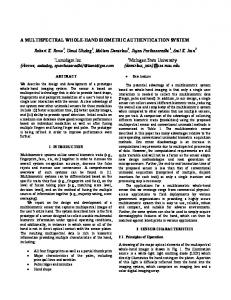
The gait identification and verification system detailed in this work shares the typical architecture (see Figure 2.1) with all other biometric systems. More generally formulated, it is a pattern recognition system. It works in two phases: the learning phase (enrolment), where several gait patterns are taken from the user; these are then pre-processed to enter the feature extraction block, where a set of measurements is performed. With the features extracted, the data reduction block determines the user’s template that is stored, for later reference, either in a central database or on a portable storage media together with the user’s ID. In the authentication (verification) phase, a single gait sequence is taken, pre-processed, and entered in the feature extraction block. This single set of features is compared to the template previously stored, obtaining a ratio of likeliness to verify the user’s claimed identity.

2.3 Identification vs. Authentication

19

Authentication Phase (verification)

Data Acquisition

Data Acquisition

Feature Extraction

Multiple Tries

Learning Phase (enrolment)

Feature Extraction

Data Reduction

Data Reduction

ID

(ID,template)

User Template Database

template

Classification

Accept

Reject

Figure 2.1: Typical architecture of a biometric authentication system.

2.3

Identification vs. Authentication

As has already been shown in the previous section, all biometric systems can be operated in two different modes: identification and authentication. In identification systems, a biometric signature of an unknown person is presented to a system. The system compares the newly acquired biometric signature to a database of biometric signatures of known individuals. This is called a “one-to-many” search, with the question “Do I know you?”. On the basis of the comparison, the system reports the probable identity of the unknown person from this database in the form of a list of likely candidates. Systems that rely on identification include those that the

20


police uses to identify people from fingerprints2 and mug shots. Civilian applications include those that check for multiple applications by the same person for welfare benefits and driver’s licenses. In authentication systems, a user presents a biometric signature and a claim (“I am user X”) that a particular identity belongs to the biometric signature. This is called a “one-to-one” search, with the question “Are you who you claim to be?”. Authentication is basically a binary classification problem, where the algorithm either accepts or rejects the claim. Alternatively, the algorithm can return a confidence measurement of the claim’s validity. Authentication applications include those that authenticate identity for physical access control of secure buildings or logical access control as used for cash dispensers. Because the claimed identity of a person presenting herself or himself for authentication is known in advance, the database search time is much faster than in identification and a matter of milliseconds rather than seconds. The quality requirements for authentication systems are generally weaker compared to identification systems, since not all people need to be differentiable. Just the probability of a missauthentications has to be small.

2.4

Physiological and Behavioural Characteristics

As can be seen in the biometric typology chart, Figure 2.2, human biometric characteristics can be separated into two different categories: the physiological and the behavioural traits. The physiological characteristics are relatively stable, such as a fingerprint, hand silhouette, iris pattern, blood vessel pattern of the retina, or DNA fingerprint. Those biometric traits are essentially fixed and do not change over time. On the other hand, behavioural characteristic are more prone to changes depending on factors such as aging, injuries, or even mood. The most common behavioural characteristic used today is the signature, although not in biometric systems. Other possible behaviours that can be used are how one speaks, types on a keyboard, or walks. Because 2 The AFIS (automated fingerprint identification system) systems are widely used in law enforcement.

2.4 Physiological and Behavioural Characteristics

21

Biometrics

Physiological Biometrics

Behavioural Biometrics

Hand

Eye

Voice

Gait

Face

Fingerprint

Signature

Keystroke

Ear Shape

DNA

Multimodal (Combination)

Figure 2.2: Typology of Biometric Methods. of the inevitable modest variations of all behavioural traits, many systems use an adaptation mechanism to update the reference template in order to compensate for slight changes of the biometric trait over time. Generally, behavioural biometrics work best with regular use. There are important differences between physiological and behavioural methods. First, the degree of intra-personal variation in a physiological characteristic is smaller than in a behavioural characteristic. Apart from injuries the iris pattern remains the same over time, whereas speech characteristics change and are influenced by many factors, e.g. the emotional state of the speaker. Developers of behaviour based systems, therefore, have a harder job in compensating for those intra-personal variations. Second, due to the intra-personal variations of behavioural methods, their discriminatory power (“How many distinguishable persons are there?”) is generally smaller than for physiological methods.

22


2.5

Living Person

While the term Living Person appears obvious, it is nevertheless important to explain it. A common question asked by newcomers to the field of biometrics is “Can’t biometric fingerprint systems be fooled by fake fingers made out of latex or by fingers that were cut off a living person?” The answer is that many but not all devices include measures to determine whether there is a live characteristic being presented or not. The methods are sometimes ingenious but usually simpler than one would expected. Face recognition systems for example often try to detect the blinking of the eyelid in order to differentiate a real face from a picture. However, most of those systems can be by-passed relatively easy by cutting a hole in a photograph and then holding it in front of the intruder’s face. This way the blinking of the intruder’s eyelid is detected but the image of the photograph is taken as the face. A different approach chosen by many commercial systems3 is to combine face recognition with a behavioural characteristic such as voice or lip movement. Although it is quite feasible to combine fingerprint detection with a different behavioural characteristic such as lip movement, a different approach is normally chosen to determine the living status of the user. Today’s modern fingerprint detection systems try to either measure the oxygen (O2 ) or carbon dioxide (CO2 ) level and its change over time in the finger’s blood stream. One of the main advantages of most behavioural biometric methods is that the living person detection is intrinsic, i.e. an integral part of the method, and no special measures need be taken. Possible examples include hand signature and gait recognition systems, but not speech, although a very popular behavioural characteristic, as it can be easily recorded. However, it is obvious that you cannot steal somebody’s signature by chopping off his or her hand.

2.6

Performance Measures

Performance statistics for identification systems differ substantially from those for authentication applications. The main performance measure 3 e.g.

BioID http://www.bioid.com/

2.6 Performance Measures

23

for identification systems is its ability to identify a biometric signature’s owner. More specifically, the performance measure equals the percentage of queries in which the correct answer is the top match. On the other hand, the performance of an authentication system, is commonly characterised by two error statistics: the False Reject Rate (FRR) also called Type I Error and the False Accept Rate (FAR) also known as Type II Error. These error rates come in pairs; for each False Reject Rate there is a corresponding False Accept Rate and vice versa, see Figure 2.3. These error rates are defined as follows FAR(λ) =

Number of False Accepts Number of Impostor Accesses

(2.1)

Number of False Rejects . Number of Client Accesses

(2.2)

and FRR(λ) =

A false accept status occurs when a system incorrectly approves an identity and a false reject status occurs, when a system incorrectly denies an identity. In a hypothetically perfect biometric system, both FAR and FRR would be zero. Unfortunately, biometric systems are not perfect, and the system operators must determine what trade-offs they are willing to make and set the variable security level appropriately, to attain the desired balance of FAR and FRR. If the security level is increased to make it harder for impostors to gain access, it will also become harder for authorised people to get access, i.e. as FAR decreases, FRR increases. Conversely, if the security level is decreased to make it easier for rightful people to gain access, then it will also be more likely that an impostor may slip through, i.e. as FRR decreases, FAR increases. The point at which these two curves intersect (see Figure 2.3) is generally referred to as the Equal Error Rate (EER), or the rate at which the number of people who are incorrectly accepted and incorrectly rejected is equal. Generally the lower the EER the better the biometric system. Table 2.1 on page 27 summarises EER values of two popular commercially available biometric systems. The EER is a parameter that gives valuable information about the quality of a biometric product or method. However, this information is generally not sufficient. A related but more specific quality measure was

24


Error Rate 100 [%]

FAR(¸)

FRR(¸)

Type II Error (FAR)

Type I Error (FRR)

EER+¢ A EER 0

¸0

¸EER

Weak

¸1 Strong

Security Level ¸

Figure 2.3: Plot of the dependencies of FAR, FRR from the security level. suggested by Lassmann et al. in [Lassmann98], that obtains closer information by determining how fast the two error rate functions FAR(λ) and FRR(λ) increase when moving the security level λ away from the optimal λEER point.

2.6 Performance Measures

25

For this purpose, a fixed value ∆ =5 % is considered and the size of the zone where FAR(λ) and FRR(λ) are both below EER + ∆ is calculated. Figure 2.3 shows the two curves for FRR and FAR with the crossover point at the EER. The area A between the horizontal line for EER + ∆ and the two curves represents the measurement for the discriminatory power and can be calculated with

λZ EER

A = (EER + ∆)(λ1 − λ0 ) −

Zλ1

FAR(λ)dλ − λ0

FRR(λ)dλ.

(2.3)

λEER

In practical applications it is often difficult to determine an adequate security level λ. Many biometric systems show substantial FAR and FRR deviations for only small changes from the theoretically optimal λEER . This makes it difficult to fine-tune the security level λ. However, methods with a large A are less prone to minute changes in λ and are thus more robust and have a larger discriminatory power. Yet another method to characterise the overall performance of a biometric authentication system is the so called Receiver Operating Characteristic (ROC) depicted in Figure 2.4, which represents the FRR as a function of the FAR [Melsa78]. The optimal point is at the lower left of the plot, and curves of well performing systems tend to bunch together near this corner. An improvement to this ROC plot visualisation tool, called the Detection Error Trade-off (DET) plot, has been introduced by Martin et al. in [Martin97]. The DET plot is a non-linear transformation of the aforementioned ROC plot, see Figure 2.6 for example. It improves the visual presentation of detection error trade-off by plotting the normal deviate of the False Alarm probability, i.e. False Reject, on the horizontal axis and the normal deviate of the Miss Probability, i.e. False Accept, on the vertical axis. Figure 2.5 illustrates the Accept and Reject Score Distributions that are assumed to be normally distributed4 with a mean of µ0 , µ1 and a standard deviation of σ0 , σ1 respectively. 4 Which

is a reasonable assumption as will be shown in the results chapter.

26


Strong Security

en ts

100%

Te

ch

no

lo

gy

False Reject Rate

Im

pr

ov

em

Method 1 Method 2

EER Points

0%

¸i

False Accept Rate

nc

re as

es

Weak Security

100%

Figure 2.4: Typical ROC plot with two different biometric methods. The operating threshold λ is shown by a bold line and the two error probabilities by shaded areas. Rather than plotting those two error probabilities, as in the ROC curves, the DET plot uses the normal deviates d0 , d1 that correspond to the probabilities instead. This linear deviation scale results in a non-linear probability scale, but the advantage is that the plots are visually more intuitive. In Figure 2.6 the probabilities are shown on the bottom and left axis, whereas the standard deviations are shown on the top and right axis. The curves are moved away from the lower left when performance is high, making comparisons between different methods easier. It can also be observed that if the distribution of error probabilities are Gaussian, then the resulting trade-off curves are straight lines and the distance between the curves depicts performance differences more meaningfully than the ROC curves. There are two important things to note about the DET curves. (1) If the resulting curves are straight lines, then the underlying distribution from the system are normal. (2) Each point on the DET curve represents

2.7 Principles of Human Locomotion

27

¾0

Reject Score Distribution

¾0 d0

¹0 False Reject Probability

Accept Score Distribution

d1

¹1

¸

False Accept Probability

Figure 2.5: Distributions of the accept and reject scores, the areas under the two curves correspond to the False Reject and False Accept Rate respectively. Biometric System FaceIt (face recognition) ID-3D (hand geometry)

EER 0.68% < 0.2%

Table 2.1: Equal Error Rate (EER) of two popular biometric systems. a particular security threshold λ. In particular, the two ◦’s in Figure 2.6 indicate the λEER point for the two methods. As is the case with all biometric systems, the False Accept Rate, False Reject Rate, and Equal Error Rate heavily depend on the particular user basis used for analysis. For a given system, a well trained and enthusiastic user base will realise a much higher level of performance compared to a group of disinterested users. In the latter case, this not only affects their inherent capability to use the system correctly, but also their attitude towards the system and eventually biometrics in general.

2.7

Principles of Human Locomotion

Gait is probably the most common of all human movements, see [Harris96]. It is difficult to learn, but once learned it becomes almost subconscious as

28


Normal Deviate 3

2 Method 1 Method 2

1.5 0

20 Normal Deviate

False Accept Rate [%]

40

2.5

10 5 2 1 .5

0.5 1 1.5 2 2.5

.2 .1

3 .1 .2 .5 1 2 5 10 20 False Reject Rate [%]

40

Figure 2.6: Typical example of two DET curves from different methods. Method 1 has a better performance. long as it is not disturbed by an injury, disease (or alcohol ;-). Two abilities are essential to walking. First, the ability to maintain the equilibrium, and second locomotion, the ability to initiate and maintain a rhythmic stepping motion. Although these two abilities are essential, there are many contributing factors involved such as the skeletal system with the joints as well as the neuro-muscular system. The field of gait analysis has turned into a major tool in orthopedic medicine and became widely used for diagnostic and rehabilitation tracking purposes. Therefore, physicians need accurate knowledge of gait so that they can detect and interpret deviations from the normal gait pattern. This research showed that each individual has certain superimposed variations from the normal gait pattern that are normally ignored in orthopedic medicine. However, those minute deviations from the normal gait pattern can be used to recognise people, as will be shown in this thesis. Of course, humans can do this differentiation very well as has been shown by Cutting in [Cutting77]. They can recognise friends and other close persons


Classification Weak Moderate Strong Very strong

FAR > 5% 5% − 1% 1% − 0.3% < 0.3%

29

FRR > 7% 7% − 3% 3% − 1% < 1%

Table 2.2: Security classification of biometric systems according to their FAR and FRR. from their gait very easily, even if they do not know the rationales behind. The following paragraphs explain the basic principles of human locomotion and the corresponding terminology. However, in this thesis only bipedal walking in contrast to running is considered. In particular, the foot of the supporting extremity remains in contact with the floor until the opposite foot has made floor-contact. The definition of the gait cycle is the time between two equal events in the walking cycle, such as the heel strike of the right foot, see Figure 2.7. The gait cycle of each individual foot can then be divided into two periods: the stance and the swing period. Roughly 60% of the gait cycle the foot is in the stance and in contact with the ground. The remaining time of the gait cycle constitutes the swing period, where the foot is in the air. The double support period, where both feet are in contact with the floor occurs twice in the gait cycle. In contrast, single support is the period of time where only one foot is in contact with the ground. The gait cycle, consisting of the stance and swing periods, can be further broken down into eight sub-phases; explained here for the right leg: 1. Initial Contact: the moment when the right foot, normally with the heel, touches the floor. 2. Loading Response: the double support phase, where body weight is transferred from the left to the right leg. 3. Mid Stance: the first half of the single limb support, that begins with the lifting of the left foot and continues until the body weight is aligned over the supporting right foot. 4. Terminal Stance: begins when the right heel rises and continues until the heel of the left foot hits the ground.

30

Chapter 2. Fundamentals One gait cycle

0% Rt heel strike

50% Lt heel strike Right stance

Right swing

Left swing

Left stance

Double support Gait sub- 1 2 phases

100% Rt heel strike

Single support 3

Double support 4

5

Single support 6

7

8

Figure 2.7: Diagram showing the different phases of the walking cycle. 5. Pre-Swing: the second double support phase in the gait cycle, that begins with the initial contact of the left foot and ends with the right foot toe-off. 6. Initial Swing: begins when the right foot is lifted and ends when the swinging right foot is opposite the stance foot. 7. Mid Swing: follows the initial swing phase until the swinging right limb is in front of the body and the lower limb is vertical. 8. Terminal Swing: begins when the lower limb is vertical and ends when the foot, normally the heel, touches the floor. Human gait can not only be characterised through the aforementioned phases, but also through a handful of common parameters. The stride length, cadence and velocity are three such interrelated parameters. Commonly misused, the term step length is not synonymous to the stride length. The step length is the distance from a given floor contact point, e.g. left heel, to the same floor contact point of the other foot, e.g. right heel. The stride length, on the other hand, includes a left- and a right-step length and thus is the distance covered in one gait cycle. The cadence refers to


31

the number of steps taken per time. Finally, the velocity combines the stride length and the cadence to express the distance covered in direction of progression per unit of time. While walking, both feet exert a certain force to the floor called the Ground Reaction Force (GRF). The GRF is a three dimensional vector as can be seen in Figure 2.8. All three force components, namely the anterior/posterior Fx , the vertical Fy , and the lateral/medial Fz component, can be measured with force plates such as the commercially available Kistler plate5 . GRF

Fy

Walking direction

Fz

Fx

Figure 2.8: The force plates are able to measure all three components of the ground reaction force (GRF). Figure 2.9 shows time series of the GRF in different directions. The vertical component Fy has two bumps, hence its name, the camel-back curve, both exceeding body weight. The first occurs after the heel strike during the loading phase, and the second during the push off phase. The anterior/posterior components Fx of the GRF shows posterior forces during the first half of the stance phase and anterior forces during the second half. There is a deceleration followed by an acceleration component. The lateral/medial component is the smallest in absolute values. It is mostly medial in direction and serves for balance purposes.

5 Kistler

Instrumente AG Winterthur, Switzerland, http://www.kistler.ch

200

1000

100

500

50

0

0

0 −200

0

0.5 Time [s] (a) Fx (t)

1

−500

0

0.5 Time [s] (b) Fy (t)

1

−50

0

0.5 Time [s]

1

(c) Fz (t)

Figure 2.9: All three components of the GRF in (a) anterior/posterior, (b) vertical, and (c) lateral/medial direction in units Newton.

Chapter 3

Description of the System This chapter describes the design and implementation of the laboratory prototype biometric system using gait characteristics, built during the course of this thesis. In order to minimise costs, the biometric system is mainly composed of commercially available parts: namely, the sensors and the processing unit, which are discussed in detail in the following sections. The design and component selection was directed towards a future product taking into consideration reliability, cost effectiveness, and simplicity.

3.1

System Overview

Figure 3.1 shows the schematic diagram of the experimental arrangement used during the course of this thesis. The setup consists mainly of three components: (1) the three force plates to measure the ground reaction force, (2) the CCD-camera to capture the video sequence, and (3) the data acquisition and processing hardware. These three components are arranged around the measuring zone where all the sensors are focused to. Whilst the subjects are passing the measuring zone, the sensors acquire the biometric data. The zone occupies an area of approximately 1 m×3 m and is depicted in Figure 3.2.

33

34

Chapter 3. Description of the System

Computer

A/DC Force plates

Framegrabber CCDCamera

Figure 3.1: Experimental setup with (1) the three force plates (2) the CCDcamera and (3) the processing hardware. In order to use the biometric system, people have to pass this measuring zone. This is also the place were all the sensors are focused to capture their data. To simplify the object/background segmentation for the video sensor, the backside of the measuring zone is equipped with a white cardboard wall. Although we are using this white wall its application does not restrict the generality of the method.

3.2

Sensors

The system consists of two sensors measuring different physical properties of the walking subjects. First, the force sensor measures the ground reaction force Fy (t) perpendicular to the floor and second, the video sensor captures a side view of the passing subject. For this thesis only the Fy (t) component of the GRF was considered, since it has the strongest discriminatory power, as can be seen in Figure 7.2(b) of the Results chapter. Both sensors are connected to the I/O-board of a standard off-the-shelf personal computer (Dell OptiPlex GXi). Although the force and video data is captured at the same time, the two data streams are not synchronised in any way.

35

. .. .. .

. .. .. .

60cm

150cm

Piezo Force Sensors

White Cardboard Wall

200cm

3.2 Sensors

60cm 400cm

Figure 3.2: Diagram of the measuring zone with the sensor arrangement.

3.2.1

Force Plate

In all biomechanical tests, the persons being tested must be unaware of the measuring devices to ensure that the movements are not influenced by the instrumentation. This is mandatory to guarantee reliable and reproducible measurements. Thus, subjects should be able to walk in their own natural way. Subjects should therefore be exempted from placing exactly one foot on each of the three force plates and be free to walk with their own accustomed stride length. Furthermore, the force plates should not raise above the surrounding floor and hinder the subjects from walking naturally. To avoid all those problems, ample priority has been paid to integrate the force plates flush with the surrounding floor. The force plates raise only about 1 mm above the surrounding floor and are operated discreetly, easily, and practically invisibly. Although from the technical side, care has been taken to permit reliable ground reaction force measurements, there is one problem that can not be

36


Walking Direction Fy(t) Fz(t)

Fx(t)

Piezo Sensor & Amplifier

Figure 3.3: Schematic of a force plate. solved. It is not easy to deliberately walk naturally. During our tests, several subjects felt awkward having to deliberately walk naturally. Figure 3.3 depicts the schematic diagram of a force plate where Fx (t) is the ground reaction force (GRF) in walking direction (anterior), Fy (t) is the ground reaction force perpendicular to the floor (vertical), and Fz (t) is the exerted force vertical to the walking direction and in the plane of the floor (lateral). Although our investigation reported in [Bachmann99] indicates that both Fx (t), as well as Fy (t) contain valuable subject specific information, only the GRF perpendicular to the floor Fy (t) is used in the course of this thesis; hereafter the Fy (t) component of the ground reaction force will be abbreviated as either ground reaction force or simply Fy (t). This simplification allows drastically straightening the construction of the three force plates. The double layered floor in our lab consists of an array of wooden tiles (60 cm × 60 cm) on metal poles, see Figure 3.4(a). Three such tiles were equipped with a piezo sensor in each corner (Figure 3.4(b)), giving a total of twelve sensors. The force sensors were built with a piezo crystal PI Ceramic 155 in an integrated package with the amplifier, see Appendix C for the detailed amplifier scheme.

3.2 Sensors

(a) Double layered floor

37

(b) Piezo sensor Integration

Figure 3.4: (a) Double layered floor with (b) the force sensors. Four such sensor and amplifier pairs were integrated on one oddly shaped PCB (see Figure 3.5) that snugly fits between the metal pole and wooden tiles, as can be clearly seen in Figure 3.4(b). Due to the piezo crystal’s capacitive property, this arrangement of measuring amplifier and piezo crystal measures the temporal derivative, F˙y (t), of the ground reaction force, rather than the force itself. Figure 4.1(a) on Page 43 illustrates a sample of the data provided by the sensors. Sensor Quality: Although the construction costs of the force sensors were very low (≈ 200 CHF) they seem perfectly adequate for this application. A comparison in [Bachmann99] with force data acquired by professionals1 in a specialised gait laboratory using Kistler force plates (≈ 60, 000 CHF) did not show a significant difference in recognition quality. 1 Dr.

Peter Erhart, Rehaklinik Bellikon, Postfach, 5454 Bellikon, Switzerland

38


3.2.2

Video Sensor

The CCD video camera is the system’s second sensor used to capture characteristic gait data. To simplify the feature extraction and to increase recognition quality the users are obliged to walk fronto-parallel to the camera with a fixed white background, see Figure 3.2, and the body never occluded. This situation can be easily realised by setting the camera in an apt position. The camera used is a standard interlaced CCD-camera with a resolution of 768 × 576 of 8-bit monochrome pixels, a framerate of 25 Hz, and a motorised zoom lens (Computar H6Z0812M). To avoid the problem of moving objects and interlaced cameras, only one half-frames was used per picture, the effective resolution thus being 768 × 288. The camera was mounted on the left hand side of the subject’s walking direction at a distance and height of approximately 4 m and 1.5 m, respectively. Figure 3.6 shows an example frame of the low vertical resolution grey-scale image.

3.3

Processing Unit

The basis of the processing unit is formed by a Personal Computer Dell OptiPlex GXi with a Pentium II 200 MHz Processor, 160 MB of main memory, and two PCI bus I/O expansion cards: 1. A Data Translation, Inc. Analog/Digital-Board DT301 with 16 single ended or 8 differential analog input channels featuring 12 bit resolution each and a maximum sampling rate of 150 kSamples/s. 2. A Data Translation, Inc. Frame Grabber card DT3155 with a resolution of up to 768 × 576 pixels with 8 bit monochrome pixels, and a maximum sampling rate of 30 Frames/s. Both the video sensor and the twelve force sensors are connected directly to the appropriate I/O-cards.

(a) Top view

(b) Bottom view Tile

}

} Plugs

Amplifier Piezo Sensor

Amplifier PCB Piezo Sensor Metal Pole

(c) Schematic side view

Figure 3.5: Piezo force sensor with amplifier.

Plugs

Figure 3.6: View from the CCD-camera.

Chapter 4

Feature Extraction This chapter describes the extraction of individual features of the acquired gait data. During the development, ample priority has been given to computationally efficient algorithms.

4.1

Introduction

Numerous different ways of extracting discriminative features from gait sequences have been proposed. Despite the broad variability of the methods they can be devided into two distinct groups: (1) systems that need to locate one step or a complete gait cycle and (2) systems that do not need to locate the gait cycle within the acquired data. (1) The biometric method proposed in this thesis as well as the systems proposed in [Orr00, Little98, Huang98b] need to locate one complete gait cycle in the data stream in order to extract the characteristic feature vectors. These feature vectors are subsequently projected into a lowerdimensional feature-space, where each gait sequence is represented by one single point. The main advantage of this approach lies on the one hand in the relatively easy classification. On the other hand it might prove difficult to locate the gait cycle. (2) In contrast, the methods of the second kind [Huang98f, Huang98c, Huang98d], need not to isolate the gait cycle. Conversely, their features

41

42

Chapter 4. Feature Extraction

vary over time and thus form a trajectory in feature-space. Each gait sequence is thus projected to a hopefully periodic trajectory in the lowdimensional feature-space. Those systems generally use a HMM to recognise and differentiate people from their trajectories. The main advantage of this method lies in the fact, that it is possible the recognise people without a complete gait cycle, but the final classification is slightly more difficult compared to the previous approach. Neither of the two approaches is per se better than the other, it is merely a way to classify the various methods.

4.2

What Features Should be Used?

In order to achieve a high recognition rate, discriminative features must be extracted from the available data. From a naive point of view, it would seem obvious to try to recognise people through their stride length, walking cadence, body weight, body height, and so forth. However tempting the aforementioned features might be, they are not ideal for a biometric system. In fact, they are highly insecure due to their static nature, that allows an impostor to easily mimic them; e.g. an impostor can easily adjust his body weight, stride length, and cadence to match that of a legitimate user and try to gain access to a restricted area. Conversely, the dynamic properties of human gait are far more difficult to imitate, since they depend on physiological properties of the user’s body, such as bone structure. The use of dynamic properties of human gait is therefore considered in this thesis.

4.3

Force Features

As already described in the preceding chapter, the piezo force sensors measure only the derivative ground reaction force perpendicular to the floor F˙y (t), see Figure 4.1(a). With a simple numerical integration one can determine the ground reaction force Fy (t). Figure 4.1(b) shows an example of the ground reaction force with its well-known camel-back shape.

43

Ground Reaction Force (GRF)

4.3 Force Features

d/dt(Ground Reaction Force)

Plate 1 Plate 2 Plate 3

0

1

2 3 Time [s] (a)

d F (t) dt y

4

5

0

1

2 3 Time [s]

4

5

(b) Fy (t)

Figure 4.1: Sample profile of (a) the vertical derivative GRF and (b) the vertical GRF of three consecutive steps. It is obvious from the phase plane graphs1 depicted in Figure 4.2 that the ground reaction force Fy (t) contains characteristics that could be used as a biometric. In particular, the phase plane plots show large similarities among the same subject but differ substantially for separate subjects. In our research reported in [Bosshard98] many different methods to extract characteristic features from the acquired GRF data have been tried. First, geometric properties extracted from the vertical GRF component were investigated, see Figure 4.1(b). In particular the area under the camel-back curve, the average body weight, the amplitudes of the heal strike and the toe-off peak, the elapsed time between the heal strike and toe-off peak, the number of local minimas of the camel-back curve, and the elapsed time for one step. Similar parameters were also proposed by Orr and Abowd in their publication [Orr00]. However, the extracted characteristics had only a very limited discriminatory power and the class separability was poor. Second, geometric parameters extracted from the phase plane graphs as depicted in Figure 4.2 were examined. Namely, the area within the curve, the position and area of the small loop, the maxima/minima in x- and y-direction, the center of gravity, as well as the shape of the parametric plot approximated with fourier descriptors. But 1 The

ground reaction force Fy (t) plotted against its derivative F˙y (t)

44


0

0 −0.5

−0.5 −100

−50 GRF

0 −0.5

−100

0

(a) Subject A

−50 GRF

0

−100

(b) Subject B

−0.5

0 −0.5

−100

−50 GRF

(d) Subject A

0

0

0.5 d/dt GRF

0

−50 GRF

(c) Subject C

0.5 d/dt GRF

0.5 d/dt GRF

0.5 d/dt GRF

0.5 d/dt GRF

d/dt GRF

0.5

0 −0.5

−100

−50 GRF

0

(e) Subject B

−100

−50 GRF

0

(f) Subject C

Figure 4.2: The parametric phase plane graphs of the ground reaction force (Fy (t), F˙y (t)) suggests that the GRF contains substantial individual characteristics. it proved very difficult to reliably extract parameters from the phase plane graphs. In [Bachmann99] we proposed the Power Spectral Density (PSD) of F˙y (t) as the characteristic feature, see Figure 4.3 for an example. The empirical investigation of the different feature extraction methods showed the best performance for the windowed2 Power Spectral Density (PSD) of the derivative ground reaction force F˙y (t). In particular, the 0 − 20 Hz frequency band is utilised to characterise subjects zforce = PSD0−20Hz (F˙y (t)).

(4.1)

Analysis of the ground reaction force, from gait data acquired at the Gait Laboratory in Bellikon, showed a slightly inferior discriminatory power for the Fx (t) and the Fy (t) component. Refer to Section 7.2 on Page 82 and Figure 7.2(b) for more details. 2 Hanning

window

45

Energy

4.4 Video Features

0

5

10 15 Frequency [Hz]

20

Figure 4.3: Sample power spectral density of the derivative of the ground reaction force F˙y (t).

4.4

Video Features

As mentioned earlier, the video camera is the second sensor used to capture characteristic gait data. It acquires for each gait sequence a 2 second video clip at a frame rate of 25 frames/s, i.e. fifty images I1 ...I50 . Additionally, the image I0 of the static background is grabbed, that subsequently eases body/background segmentation. In order to efficiently extract characteristics based on the subject’s silhouette and its variation in time it is essential to eliminate irrelevant background from each image. Thus, preprocessing of the image data is necessary. Figure 4.4 shows the preprocessing steps as required to extract the distinctive features of the human outline.

4.4.1

Image Segmentation

The first step of video feature extraction is the image segmentation, where the subject’s body is separated from the background by eliminating unrelated information. This is crucial for computationally efficient and accurate feature extraction.

46


Image Sequence I1

I2

I3 .

..

Image Segmentation

. * I* . . I*1 I 2 3 Stride Extraction

. . . . . . Hk+n-1 Hk Hk+1 Histogram Features

v1

v2

Temp.Templ. Features

v3

v4

Figure 4.4: Outline of the video feature extraction subprocesses. First the static background I0 is subtracted from every image I1 ...I50 . This already eliminates a major part of insignificant image data. Subsequently, these image differences are binarised with the iterative Markov thresholding method described in [Li95]. After locating the silhouette in the binarised images, they are cropped and scaled to a standard height of ∗ 200 pixels resulting in I1∗ ...I50 . The aspect ratio is kept constant when the height is normalised. Figure 4.5(a) shows the binarised and scaled image of the sample image shown in Figure 3.6.

4.4.2

Stride Extraction

In order to get reliable, stable and distinctive features the intra-personal variations of the features should be minimised. This can be achieved by ensuring that all gait features are always extracted from a complete gait cycle for every individual gait sequence; thus a left-right-step or a rightleft-step sequence respectively.

4.4 Video Features

47

(a)

(b)

Figure 4.5: (a) Segmented sample image Ii∗ with the corresponding (b) horizontal pixel histogram Hi . ∗ To locate this gait cycle in the image sequence I1∗ ...I50 the horizontal 3 pixel histogram Hi (∀ i = 1...50) is calculated for all the segmented and binarised images; see Figure 4.5(b) for a histogram example.

Since human gait is per se a periodic movement, the time series of histograms H1 ...H50 must be periodic as well. It is thus possible to locate the beginning and end of the gait cycle by least square fitting a periodic function4 at a particular height, such as the hip or knee, into the histogram series. This yields a sequence of n histograms Hk ...Hk+n−1 containing the complete gait cycle.

4.4.3

Histogram Features

Once the gait cycle is located, three different types of features (v1 , v2 , v3 ) are extracted from this subsequence Hk ...Hk+n−1 of histograms. Namely the average histogram vector

v1 :

µ ¯=

k+n−1 1 X Hj n j=k

3 The 4 The

number of white pixels in each of the 200 rows of the image. sine function was chosen for the course of this thesis.

(4.2)

48


with a size of 200 dimensions. The histogram variance vector

v2 :

σ2 =

k+n−1 1 X (Hj − µ ¯)2 n

(4.3)

j=k

with a size of 200 dimensions and finally the two-dimensional Fast Fourier Transform (FFT) v3 :

˜ = FFT2([H ~ k , ..., H ~ k+n−1 ]). H

(4.4)

with a size of 1, 000 dimensions. Together the three feature vectors span a hyper-space with 200 + 200 + 1000 = 1, 400 dimensions.

4.4.4

Temporal-Template Features

Davis et al. proposed in [Davis97, Davis99] a method to recognise human actions and gestures using two different variants of temporal-templates: (1) a binary motion-energy image (MEI) which represents where motion has occurred in an image sequence and (2) a motion-history image (MHI) which is a scalar-valued image where intensity is a function of recency of motion. The temporal-template feature used in the course of this thesis is a representation of how the person moves during one complete gait cycle, see Figure 4.6 for a sample. The pixel intensity in this temporal-template represents the number of pixels set in the binarised image sequence Ii∗ . The temporal-template can thus be calculated by summing up all the segmented images Ii∗ of the gait cycle i = k...k + n − 1

A=

k+n−1 X

Ii∗ .

(4.5)

i=k

As has been explained in Section 4.2, it is not recommended to try to recognise subjects through their stride length or their height directly. The recognition can be achieved in a better way by normalising the temporaltemplates to a standard width and height, the normalised temporaltemplate size thus being 256 × 768 pixels respectively. Figure 4.6(a) shows an example of such a normalised temporal-template. To further reduce

4.5 Summary

49

5

50

10 100 15 150

20

200

25 30

250 200

400

600

20

(a)

40

60

80

(b)

Figure 4.6: (a) Example temporal-template of a complete gait cycle and (b) it’s 8 × 8 subsampled version. data dimensionality the temporal-template is 8 × 8 subsampled, see Figure 4.6(b)

v4 :

SUBSAMPLE8×8 (A) = SUBSAMPLE8×8

k+n−1 X

! Ii∗

.

(4.6)

i=k

Thus the resulting feature vector v4 will have a size of 96 = 3072 dimensions.

4.5

256 768 8 8

= 32 ×

Summary

In this chapter the extraction of individual features of the acquired gait data was shown. The first section explains the advantages and disadvantages of the two different methods to extract characteristic features. The second section details why dynamic features are of particular interest for a biometric system. The third section describes the extraction of the FFT

50


Feature Type Force plate Histogram-mean Histogram-variance Histogram-FFT Temporal-template Total

fp v1 v2 v3 v4

Captured Data 6 kB 10 MB ” ” ” 10 MB

Extracted Features 128 Reals 200 Reals 200 Reals 1000 Reals 3072 Reals 4600 Reals

Table 4.1: Size of the captured input data and the number of extracted features thereof. features from the force plates, whereas the fourth section illustrates the extraction of the various features from the video sensor. The force feature extraction method uses the Power Spectral Density of the derivative ground reaction force. Investigations showed the best classification of the subjects in the frequency range of 0 − 20 Hz. For the extraction of the video features three different characteristics of the changing subject silhouette were used. The fourth temporal-template characteristic combines the changing silhouette as well as its forward motion. Table 4.1 summarises the amount of captured input data and the number of extracted features from this data. The original data size of more than 10 MB was reduced to 4600 Reals with 8 Bytes each. Thus, the five feature types span a hyper-space with 4600 dimensions.

Chapter 5

Transformation 5.1

Introduction

As seen in the previous chapter, several feature types are extracted from the ground reaction force and video data of every gait sequence with a total of 4, 600 dimensions. In principle it is possible to directly classify the different subjects within this high dimensional feature-space. However, large feature vectors are difficult to handle, computationally inefficient, and impractical for storage. Besides, not all of the previously extracted features have the same discriminatory power, some even contain random values. Since not all of them are equally relevant for the recognition task the less relevant ones can be safely neglected. Thus, it is possible to reduce data dimensionality without losing or, even better, improving class separability. One well known general method to perform such a transformation is the Principal Component Analysis (PCA) [Jolliffe86]. However, in this chapter a novel variant of the Generalised Principal Component Analysis (GPCA), developed in the framework of this thesis, is proposed to project the feature vectors into a lower dimensional feature-space. Typically, the first few dimensions (< 10) are sufficient for classification.

51

52

Chapter 5. Transformation

5.2

Linear Transformation

Each one of the next three sections describes a different approach to transform the high dimensional feature-space to a lower dimensional featurespace without losing class separability. Assume there are c training classes, i.e. persons, to be learned. Each class represents various training sequences of a single person, where w ~ i,j is the j-th training sequence of class i each with p features. Ni is the number of training sequences in class i. The total number of training sequences is then given by

N = N1 + N2 + ... + Nc =

c X

Ni .

(5.1)

i=1

The whole training set is represented by W = [w ~ 1,1 , ..., w ~ 1,N1 , w ~ 2,1 , ..., w ~ 2,N2 , w ~ c,1 , ..., w ~ c,Nc ]0

(5.2)

where w ~ i,j is a vector of n features. At first, all feature vectors of the training set w ~ i,j are z-transformed 1 with ~xi,j =

w ~ i,j − µ ~ , ~s

∀ i, j

(5.3)

where the mean feature vector of the set is defined by

µ ~=

c Ni 1 XX w ~ i,j N i=1 j=1

(5.4)

and the standard deviation respectively v u Ni c X u1 X ~s = t (w ~ i,j − µ ~ )2 . N i=1 j=1 1A

z-transformed distribution has a mean of 0 and a standard deviation of 1

(5.5)

5.2 Linear Transformation

53

Thus, the new z-transformed training set can be rewritten as X = [~x1,1 , ..., ~x1,N1 , ~x2,1 , ..., ~x2,N2 , ~xc,1 , ..., ~xc,Nc ]0 .

5.2.1

(5.6)

Principal Component Analysis

The Principal Component Analysis 2 (PCA) is based on statistical properties of the vector representations and is a means to extract a few characteristic features from a high-dimensional example data set. This quality makes it an interesting tool for this application. It is basically a systematic method to reduce data dimensionality of the input space by projecting the data from a correlated high-dimensional space to an uncorrelated lowdimensional space. PCA uses the eigenvalues and eigenvectors generated by the correlation matrix to rotate the original data coordinates along the direction of maximum variance. When ordering the eigenvalues and their corresponding eigenvectors, or Principal Components (PC), in decreasing order of magnitude, the first Principal Component (P C1 ) accounts for the largest variance in the original data set3 , the second orthogonal Principal Component (P C2 ) for the largest remaining variance and so forth. Over the years, several techniques from numerical analysis have been suggested to efficiently compute Principal Components (see Chapter 3.5 in [Jolliffe86]). Probably the most popular method is based on results from matrix theory, namely the Singular Value Decomposition (SVD), which is relevant to PCA in several aspects. Given the training set matrix X, of dimension N × p, and rank r, it can be rewritten using SVD as X =U ∗S∗V0

(5.7)

where U is an orthogonal N ×r matrix, V is an orthogonal p×r matrix with the eigenvectors4 [e1 , ..., er ], and S is a r × r diagonal matrix containing the square roots of the eigenvalues of the correlation matrix X 0 X, and hence the variances of the Principal Components. The r eigenvectors, i.e. Principal Components of matrix V , form an orthogonal basis that spans a new vector space, called feature-space. Thus, 2 This transform also is commonly referred to as Eigenvector, Hotelling, or discrete Karhunen-Lo` eve transform. 3 I.e. it points in the direction of the largest variance in the original data set. 4 In PCA theory commonly referred to as Principal Component or PC respectively.

54


each vector ~xi,j can be projected to a single point in this r-dimensional feature-space. However, according to the theory of PCA for highly correlated data, each training set vector can be approximated by taking only the first few k, where k ≤ r, Principal Components e1 , ..., ek . This partial set of k PCs span a lower-dimensional eigenspace in which ~yi,j are the projections of the original feature vectors ~xi,j given by

PC3

10 0 −10 −20 −30 −10

0

20 10

20 PC1 30 (a)

0 −20 PC2

Percent. of Total Variance [%]

~yi,j = [e1 , ..., ek ]0 ~xi,j .

(5.8)

60 50 40 30 20 10 0

2

4 6 8 10 12 Factor Number k (b)

Figure 5.1: (a) Sample feature-space of the first three Principal Components after the PCA transformation of a histogram-mean video feature set. (b) Eigenvalues of the correlation matrix. Figure 5.1(a) shows an example feature-space with the first three PCs and in Figure 5.1(b) the eigenvalues of the corresponding correlation matrix. Each class in the feature-space is represented with a different symbol. Preferably the different training sequences for each class form a cluster. However easy and efficient PCA might seem, one big disadvantage remains. Namely, the “a priori” known class membership is not considered when computing the transformation. Useful information is thus neglected which subsequently results in lower class discrimination. The following two sections describe two different enhancements that use the information available at the training stage to gain better class separability.


5.2.2

55

Canonical Space Transformation

Huang et al. proposed in [Huang98c] to extend the PCA with a subsequent Canonical Space Transformation that incorporates the class membership information to increase class separability. Given the PCA transformed vectors described in the preceding section, thus ~yi,j is the j-th vector in class i with k features, then the mean vector of the entire set can be calculated with

µ ~y =

c Ni 1 XX ~yi,j N i=1 j=1

(5.9)

and the mean vector of class i is represented by

µ ~i =

Ni 1 X ~yi,j . Ni j=1

(5.10)

Let the correlation matrix Cw denote the within-class scatter matrix and the correlation matrix Cb denote the between-class scatter matrix, thus

Cw

=

c Ni 1 XX (~yi,j − µ ~ i )(~yi,j − µ ~ i )T N i=1 j=1

(5.11)

Cb

=

c 1 X Ni (~ µi − µ ~ y )(~ µi − µ ~ y )T N i=1

(5.12)

where Cw represents the mean of within-class vectors distance and Cb represents the mean of between-class vectors distance. The objective is to minimise the within-class scattering Cw and maximise between-class scattering Cb simultaneously, that is to maximise the criterion function known as the generalised Fisher linear discriminant function [Devroye96] and given by

J(W ) =

W T Cb W . W T Cw W

(5.13)

56


The ratio is maximised by the selection of features W if ∂J = 0. ∂W

(5.14)

According to [Fukunaga72], Equation 5.14 can be solved and represented as Cb wi∗ = λi Cw wi∗

(5.15)

−1 Cw Cb wi∗ = λi wi∗

(5.16)

and thus we get

−1 where λi and wi∗ are the eigenvalue and eigenvector of Cw Cb . The Canonical Space Transformation can be realised by solving the generalised eigenvalue Equation 5.16. The eigenvectors wi∗ form an orthogonal basis that spans a new vector space, called canonical space. Thus, each vector ~yi,j can be projected to a single point in this canonical space. As in PCA, each training set vector can be approximated by taking only the first few k eigenvectors w1∗ , ..., wk∗ . This partial set spans a lower-dimensional space in which ~zi,j are the projections of the original feature vectors ~yi,j given by

~zi,j = [w1∗ , ..., wk∗ ]0 ~yi,j .

(5.17)

By merging the two linear transformations of Equation 5.8 and Equation 5.17 each image can be directly projected into one point in the lowdimensional canonical space by ~zi,j = [w1∗ , ..., wk∗ ]0 [e1 , ..., ek ]0 ~xi,j .

(5.18)

Figure 5.2(a) shows an example feature-space with the first three dimensions, i.e. k = 3, and Figure 5.2(b) depicts the eigenvalues of the −1 Cb . corresponding matrix Cw The Principal Component Analysis is useful to reduce the dimensionality of each gait template by projecting it from a highly correlated highdimensional space to an uncorrelated low-dimensional space. However,

57

PC3

10 0

−10 −20 −10

10

0

10 PC1 20 (a)

0 −10 PC

2

20



60 50 40 30 20 10 0

1 2 3 4 5 6 7 8 9 10 Factor Number k (b)

Figure 5.2: (a) Sample feature-space of the first three (k = 3) Principal Components after the CST transformation. (b) Eigenvalues of the correlation matrix. PCA is not sensitive to class structure in the gait data. Thus, PCA is used to reduce the template dimension in the first stage. In the subsequent second stage, CST then improves the class separability by maximising the between-class variations whilst minimising the within-class variations. It can be clearly seen in Figure 5.2(a) that all the gait sequences of each class form a nice cluster. Thus, CST has drastically improved class separability. The first data reduction with the PCA is essential to circumvent the singularity problem that occurs in the CST, when the number of elements p in the feature vectors is higher, than the number N of feature vectors in the training set.

5.2.3

Generalised Principal Component Analysis

The basic technique of the Principal Component Analysis has been adapted in many different ways. One such extension is the Generalised Principal Component Analysis (GPCA). This section describes the novel GPCA variant developed in the framework of this thesis which is equal to a PCA but ~ for every feature. In the special case with an additional weighting term ψ

58


~ = ~1 the GPCA is equivalent to the where the weighting term equals ψ PCA. Similar to the definition of the Principal Component Analysis in Equation 5.7, the base equation of the Generalised Principal Component Analysis can be written as

~ = U ∗S∗V0 X ∗ diag(ψ) Xψ = U ∗ S ∗ V 0

(5.19) (5.20)

~ the where X is the matrix with the training set feature vectors and ψ weighting vector. The left hand side of Equation 5.19 is known; the equation can be solved with a Singular Value Decomposition (SVD), where V contains the eigenvectors, i.e. the Principal Components, and the diagonal matrix S contains the square roots of the eigenvalues of the correlation matrix Xψ Xψ0 , and hence the variances of the Principal Components. ~ On the one hand, it is But how to choose the weighting term ψ? obvious that individuals can be best recognised with features that remain virtually constant for every trial of the individual. On the other hand, class separability increases, if the feature varies a lot within the group of individuals. Translated into a more mathematical formulation: features having a small variance within the class, i.e. person, but with a large variance among the different classes should be amplified. In practice, the “a priori” knowledge of the class membership can be used to calculate ~ As will be shown, including this knowledge is the weighting vector ψ. computationally efficient and greatly improves classification performance. Let µ ~ i be the mean feature vector of the i-th class defined by

µ ~i =

Ni 1 X ~xi,j Ni j=1

(5.21)

and the mean µ of all µ ~ i is defined by c

µ=

1X µ~i c i=1

(5.22)


59

then a measure for the between-class scattering, strictly speaking the variance, can be written as c

1 X (~ µi − µ)2 c − 1 i=1

v~b =

! 32 (5.23)

and the within-class scattering respectively

v~w =

Ni c X X

(~xi,j − µ ~ i )2 .

(5.24)

i=1 j=1

Since all features with a small scattering within the class, but a large scattering between the classes, should be amplified, the weighting vector ~ can be calculated as the ratio of Equation 5.23 and Equation 5.24 ψ ~ = v~b = ψ v~w

1 c−1 c P

c P

2

32

(~ µi − µ)

i=1 Ni P

(5.25)

(~xi,j − µ ~i

)2

i=1 j=1

where the numerator is a measure for the scattering between the classes and the denominator is a measure for the scattering within the classes, i.e. persons   ~ = Xψ = X ∗ diag(ψ)  

µ ~ 01 µ ~ 02 .. . µ ~ 0c

   ~  ∗ diag(ψ). 

(5.26)

To further reduce the computational load, only the weighted class means µ ~ i are used in Equation 5.26 to calculate the transformation. Similar to the theory of PCA, Equation 5.19 can be rewritten and solved with the Singular Value Decomposition of Xψ Xψ = U ∗ S ∗ V 0

(5.27)

60


PC3

5 0 −5

−10 −10

−5

0 PC1

5

5 (a)

10

0 −5 PC 2

15


where V represents the new orthogonal basis, called the feature-space transformation matrix. Figure 5.3(a) depicts the first three (and most significant) dimensions of a sample feature-space of a set of histogrammean µ ¯ feature vectors. Each cluster in the feature-space represents one class, i.e. person.

60 50 40 30 20 10 0

1 2 3 4 5 6 7 8 9 10 Factor Number k (b)

Figure 5.3: (a) Sample feature-space of the first three Principal Components after the GPCA transformation of video feature set. (b) Eigenvalues of the correlation matrix.

5.3

How Many Principal Components?

The major goal for using the Principal Component Analysis was to replace the p-dimensional feature-space with a much smaller m-dimensional feature-space, which nevertheless discards only little information. For most empirical data, a large part of the total variance can be sufficiently approximated with the first few Principal Components only. But how many Principal Components are needed? In literature, several “rules of thumb” have been proposed, see Chapter 6 in [Jolliffe86] or Section 15.4 in [Bortz93] for good compilations of the various methods.

5.3 How Many Principal Components?

61

Kaiser-Guttman (KG): The idea behind the Kaiser-Guttman rule, see Chapter 15.4 in [Bortz93], is that if all p variables of the feature-space are independent, then the PCs are the same as the original variables and all have unit variances5 . Thus any PC with a variance of less than one contains less information than the original variables and is therefore not worth retaining. Factor k Eigenvalue

1 87.2

2 29.2

3 13.3

4 8.2

5 6.5

6 6

7 3.7

8 3

9 2.3

10 0.0

Table 5.1: Eigenvalues, i.e. variances, of the Principal Components depicted in Figure 5.3. In other words the KG-rule retains only those PCs whose variances, i.e. eigenvalues, are ≥ 1. For the example in Table 5.1 it would thus retain 9 Principal Components. For large variable spaces p, the KG-rule usually retains too many PCs. It is nevertheless a useful and simple rule to derive an upper limit of PCs to be retained. Cumulative Variance: Probably the most obvious criterion for choosing m is to select a cumulative variance threshold t, say t = 90%, of the total variance that the first m PCs should account for. The required number of PCs is then the smallest value of m for which the chosen percentage is exceeded. From PCA theory, follows that the variance of the i-th PC, i.e. eigenvector, is equal to its corresponding eigenvalue λi . The total variance Tp can thus be calculated with

Tp =

p X

λi .

i=1 5 Because

they were initially z-transformed, see Equation 5.3

(5.28)

62


Since PCs are successively chosen to have the largest possible variance, the obvious definition of the cumulative variance accounted for by the first k PCs is therefore

tk =

k 1 X λi Tp i=1

(5.29)

and m is the smallest value k for which tk > t.

Cumulative Variance tk [%]

100

t=90% 80 60 40 20 0

2

4 6 8 Factor Number k

10

Figure 5.4: Cumulative variance graph. Figure 5.4 depicts the cumulative variance of the example in Figure 5.3. The dotted line represents a threshold t of 90%. Thus, only the first k = 5 PCs are needed to account for more than 90% of the total variance. This in contrast to the recommended nine Principal Components of the KG-rule described in the previous paragraph. Scree Test: The Scree Test which was described and named by Cattell (1966) involves looking at the plot of the eigenvalues λi against the factor number k, see Figure 5.3(b) for an example. The Scree Test involves a certain degree of subjectivity, because there is no formal numerical cut-off based on the λi . The idea behind the Scree Test, is that important factors have a large eigenvalue and as such also explain a large part of the total variance. If the eigenvalues are plotted, they form a curve heading towards almost

5.4 Comparison

63

0% variance explained by the last dimension. Thus, the point at which the curve levels out, sometimes referred to as the “elbow”, indicates the number of useful PCs which are present in the data. For the example, depicted in 5.3(b), the Scree Test suggests to retain the first six Principal Components.

5.4

Comparison

Now that three different methods have been introduced to reduce the data dimensionality of the feature vectors, the remaining problem is the quantification of their performance. It is unquestionably difficult to get an objective quality estimation by merely looking at the 3D cluster plots, e.g. Figure 5.1. The following section proposes a novel method to quantify the cluster quality based on the Mahalanobis Norm and subsequently compares the three different methods. Finally, the three transformations are compared according to their computational expenses.

5.4.1

Cluster Quality Assessment

As has already been mentioned, the quality assessment for the three transformations (PCA, CST, and GPCA) is not trivial. A similar problem occurs in cluster analysis that attempts to assess the relationship among patterns of the data set by organising the patterns into groups or clusters such that the patterns within a cluster are more similar to each other than are patterns belonging to different clusters. However, the engineering literature has paid very little attention to cluster quality issues, limiting the effort to present new clustering algorithms or dimensionality reducing methods. This section suggests a simple yet effective method to quantify the cluster quality.

64


Y2 ,y 2,

1

Axis2

d Y1

Y1

´´ ´ ´ ´´

d Y1,

´ y 2,1 ´ y 2,2 ´ y 2,3

y 2,3

dY

1 ,y c,1

yc,1 ´

Yc y c,3 ´ ´ yc,2 Axis1 Figure 5.5: Sample feature-space with three well separated clusters, i.e. classes (Y1 , Y2 , and Y3 ). Idea: It is obvious from Figure 5.5 that classification works best if (1) the clusters are well separated, and (2) the clusters are compact in size. The quality measure Q should therefore quantify the distance between the clusters with respect to their spreading. Additionally the quality measure should be scale invariant. The method proposes the average distance from all clusters to the other data vectors as the quality measure Q. But what distance measure suits the aforementioned prerequisites? Obviously the Euclidean norm does not, since it neglects cluster spreading and depends on scale. Conversely, the Mahalanobis norm6 removes all those limitations of the Euclidean metric and easily matches the prerequisites for a suitable distance measure. Rather than calculating the average distance, it is also possible to graphically compare different methods by sorting all distances in ascending order and plotting them in a 2-dimensional graph, see Figure 5.6 for an example. Definition: Assume there are c training classes Y1 , ..., Yc . Each class Yi represents various training sequences of a single person, where ~yi,j is the j-th vector of class i in the k-dimensional feature-space. Ni is the number 6 See

Appendix B for a detailed description of the Mahalanobis norm

5.4 Comparison

65

Method PCA CST GPCA

Quality Q 1.7 ∗ 103 3.3 ∗ 103 5.0 ∗ 103

Table 5.2: Mean mahalanobis distance of the three transformations presented in this section. of training sequences in class i. The total number of training sequences is thus given by

N=

c X

Ni

(5.30)

i=1

and the c cluster centres are given by Ni 1 X ¯ Yi = ~yi,j . Ni j=1

(5.31)

The distance dm,yi,j of the cluster centre Y¯m of class m to the training sequence ~yi,j can thus be written as dm,yi,j = ||Y¯m , ~yi,j ||

∀m, ∀~yi6=m,j .

(5.32)

Note that ||, || is the Mahalanobis norm. The quality measure Q can therefore be calculated with Q=

1 X dm,yi,j . N

(5.33)

Table 5.2 summarises the cluster quality Q for the three transformations presented in this thesis. The values were calculated with the data acquired during the course of this work. According to the table, GPCA shows the best performance. The superiority of GPCA over PCA and CST can also be seen quantitatively in Figure 5.6. The main drawback with the implementation of this cluster quality measure is computational, since calculating Q becomes computationally very expensive as N increases.

66


Log

10

Mahalanobis Distance

105

PCA CST GPCA

4

10

103 102 101 100

0

100 200 300 400 Feature−Space Point n

Figure 5.6: Plot of all sorted mahalanobis distances for the three transformations presented in this section. The GPCA shows the best performance, as it has larger mahalanobis distances than the other two methods. Additionally, it has the largest minimal distance.

5.4.2

Computational Aspects

At the very heart of all three transformations (PCA,CST, and GPCA) lies a Singular Value Decomposition. If matrix A has a size of m × n, then the computational complexity of the SVD is given by SVD(A)

:

O(m × n2 ).

(5.34)

Although all methods use the SVD, the matrix dimensions vary among them. Table 5.3 summarises the computational complexity of the various methods including a real world example. As can be seen in the last column, the GPCA method uses substantially less computational resources compared to the other two methods. The difference is roughly a factor of ν = N/c. The number of MFlops given in the Sample Figure column of Table 5.3, were used for the calculation of the corresponding sample images, i.e. Figure 5.1(a) for PCA, Figure 5.2(a) for CST, and Figure 5.3(a) for GPCA.

Method PCA CST GPCA

Computational Complexity O(N × p2 ) O(N × p2 ) + O(N × k 2 ) O(c × p2 )

Sample Figure 390 MFlops 391 MFlops 80 MFlops

Table 5.3: Comparison of the computational complexity.

Chapter 6

Fusion This chapter details the process of combining, i.e. fusing the different modalities and the subsequent classification of the result to come up with a decision.

6.1

Introduction

Fusing different biometric modalities results in a system that outperforms the different individual modalities. This is particularly true if the various modalities are not correlated. In Chapter 4, five different methods to extract characteristic features, i.e. biometric modalities, from the acquired gait data were presented. Chapter 5 then detailed on how to reduce the data dimensionality of the extracted feature vectors to a manageable size. However, the problem still remains to fuse and classify the 10-dimensional feature-spaces of the different modalities to come up with a decision whether to accept or reject the user. Different strategies such as multi-layer perceptron and decision trees have been proposed for analysing information obtained from multiple sources. The simplest technique is to form an extended feature vector, containing information from both the force and video sensors, and treat this vector as the vector output of a single source. However, this approach

69

70

Chapter 6. Fusion

is computationally expensive and it is successful only when all the modalities have comparable statistical characteristics and similar discriminatory powers. A different approach is depicted in Figure 6.1 that shows the typical architecture of a parallel multi-modal sensor fusion system, where a user claims an identity by providing a new template of his biometric trait. Each of the different N modalities has its own optimised local expert that compares the new template to the stored template associated to the claimed identity. All of them produce a match-score scorei that expresses the opinion of the local expert based on the available information. In the final stage, the global expert merges the local expert’s different opinions, i.e. match-scores, and makes a final decision whether to accept or reject that particular user. New Template

Local Expert 1 Local Expert 2

User Template Database

Local Expert N

score1 score2

Fusion

accept reject

scoreN

Figure 6.1: Principle of a parallel multi-modal fusion scheme. The parallel multi-modal sensor fusion approach as described in [Ben-Yacoub99] and as depicted in Figure 6.1 has been chosen for this work. Section 6.2 details the implementation of the local experts with the Bayes Risk Criterion and Section 6.3 describes the technology behind the global expert as used throughout this thesis.

6.2

Local Expert

To model the local experts, the Bayes Risk Criterion, see [Melsa78], has been used as subsequently described.

6.2 Local Expert

71

To explain the principle of the Bayes Risk Criterion, this section starts with the simplest class of decision problems: namely a binary decision with a single observation. The term binary decision implies that there are only two possible messages m1 and m2 in the message space and that the decision space has also only two possible elements d1 and d2 ; thus if message mi is present, then di is the correct decision. The problem is to select a decision rule such that it maps the observation space Z into the decision space in some optimal manner. Since it is a binary decision problem, the observation space Z can be divided into two disjoint decision regions Z1 and Z2 such that if the observation z ∈ Z1 decision d1 is taken and if z ∈ Z2 decision d2 is chosen.

p(z jm1)

p(z jm 2)

z Z1

Z2

Figure 6.2: Graphical representation of a binary decision rule. This requires the knowledge of the two conditional probability density functions p(z|m1 ) and p(z|m2 ) of the observations given each of the two possible messages. If the message is m1 , then the probability of receiving an observation in the range (z, z + dz) for sufficiently small dz is p(z|m1 )dz. On the other hand, if the message is m2 , then the probability of receiving an observation in the range (z, z + dz) is p(z|m2 )dz. Hence to select the more likely cause of an observation in the range (z, z + dz), one could decide d1 if p(z|m1 )dz > p(z|m2 )dz or d2 if p(z|m1 )dz < p(z|m2 )dz respectively. Cancelling the common dz yields the following simple decision rule

d(z) =

( d1

if p(z|m1 ) > p(z|m2 )

d2

if p(z|m1 ) < p(z|m2 ).

(6.1)

Figure 6.2 illustrates this simple decision rule commonly known as the Maximum Likelihood Decision Criterion.

72

Chapter 6. Fusion

There are two types of possible errors in a binary decision problem. On one hand, the type-one errors where d2 is decided when m1 is true. On the other hand, the type-two errors where d1 is decided when m2 is true. The type-one and type-two errors are also known from radar technology as the false alarm and miss probability. Translated to the common terms used in the field of biometrics a type-one error represents a person incorrectly rejected, i.e. False Rejection, and the type-two error a person incorrectly accepted by the system, thus False Acceptance. In addition to the two errors, there are also two correct decisions in a binary decision problem. One might decide d1 when m1 is present and d2 when m2 is present. In terms of the conditional probability densities these four cases can be expressed as

Z P {d1 |m1 } = P {z ∈ Z1 |m1 } =

p(z|m1 )dz

(correct)

(6.2)

p(z|m2 )dz

(type-two) (6.3)

p(z|m1 )dz

(type-one) (6.4)

p(z|m2 )dz.

(correct) (6.5)

Z1

Z P {d1 |m2 } = P {z ∈ Z1 |m2 } = Z1

Z P {d2 |m1 } = P {z ∈ Z2 |m1 } = Z2

Z P {d2 |m2 } = P {z ∈ Z2 |m2 } = Z2

The basic idea behind the Bayes Risk Criterion method is to assign a cost to each one of those correct, as well as incorrect, decisions. The Bayes Risk Criterion then tries to minimise the average total cost. Let Cij be the cost of making decision di when mj is true, then the binary decision problem has four possible costs: C11 C12 C21 C22

= = = =

Cost Cost Cost Cost

of of of of

deciding deciding deciding deciding

d1 d1 d2 d2

when when when when

m1 m2 m1 m2

is is is is

true true true true.

C11 and C22 are costs associated with correct decisions whilst C12 and C21 are costs assigned to incorrect decisions. Although it may seem strange at first to assign a cost to a correct decision, there is nothing fundamentally inconsistent in doing so.

6.2 Local Expert

73

The expected average cost B is thus given by

B = C11 P {d1 , m1 }+C12 P {d1 , m2 }+C21 P {d2 , m1 }+C22 P {d2 , m2 }. (6.6) Since P {dj , mk } = P {dj |mk }P {mk }

(6.7)

Equation 6.6 can be rewritten and the average cost becomes

B = (C11 P {d1 |m1 } + C21 P {d2 |m1 }) P {m1 }+ (C12 P {d1 |m2 } + C22 P {d2 |m2 }) P {m2 }.

(6.8)

Since for every m1 or m2 a decision has to be taken, the following equation hold

P {d1 |m1 } + P {d2 |m1 } = 1 P {d1 |m2 } + P {d2 |m2 } = 1 or

P {d1 |m1 } = 1 − P {d2 |m1 } P {d1 |m2 } = 1 − P {d2 |m2 }. Thus the average cost can be rewritten as

B =C11 P {m1 } + (C21 − C11 )P {d2 |m1 }P {m1 }+ C12 P {m2 } − (C12 − C22 )P {d2 |m2 }P {m2 } B =C11 P {m1 } + C12 P {m2 }+ Z Z (C21 − C11 )P {m1 } p(z|m1 )dz − (C12 − C22 )P {m2 } p(z|m2 )dz. z2

z2

(6.9)

74

Chapter 6. Fusion

Combining the two integrals yields

B =C11 P {m1 } + C12 P {m2 }+ Z [(C21 − C11 )P {m1 }p(z|m1 ) − (C12 − C22 )P {m2 }p(z|m2 )]dz. z2

(6.10) The Bayes decision criterion requires the selection of region Z2 so that the average cost B, as given in Equation 6.10 is minimal. Since the first two terms of the right side of the equation are independent of Z2 they are not relevant for the minimisation and can thus be neglected. The integral becomes minimal, if all the values z for which the integrand is negative, are assigned to Z2 . Therefore

(C21 − C11 )P {m1 }p(z|m1 ) − (C12 − C22 )P {m2 }p(z|m2 ) < 0

(6.11)

and thus

d2

(C12 − C22 )P {m2 }p(z|m2 ) ≷ (C21 − C11 )P {m1 }p(z|m1 ).

(6.12)

d1

Assuming that the cost for a correct decision is less than for an incorrect decision, the following inequality holds (C12 − C22 ) > 0

(6.13)

and the Bayes decision rule can be rewritten in the form of a likelihoodratio test p(z|m2 ) d2 (C21 − C11 )P {m1 } ≷ . p(z|m1 ) d1 (C12 − C22 )P {m2 }

(6.14)

6.3 Combination of Local Experts

6.3

75

Combination of Local Experts

Since, the extracted force and video features generated by the different sensors are statistically independent, Equation 6.14 can be extended to n Y pi (zi |m2 )

d2

pi (zi |m1 )

d1

i=1

≷

(C21 − C11 )P {m1 } . (C12 − C22 )P {m2 }

(6.15)

With the standard “0-1” cost function, described in [Melsa78], that assigns 0 costs to a correct decision and 1 to an incorrect decision

C11 = C22 = 0 C12 = C21 = 1

and with the assumption that both events m1 , m2 are equally likely P {m1 } = P {m2 } = 1/2, Equation 6.15 can be further simplified to n Y pi (zi |m2 )

d2

pi (zi |m1 )

d1

i=1

≷λ

(6.16)

where λ = 1. Depending on the application’s security requirements, λ can be tuned to meet a specific False Reject Rate, or False Accept Rate respectively. To model the likelihood functions pi (zi |m) a normal distribution was assumed [Berger85] and its parameters µi and σi were estimated from the training set.

76

6.4

Chapter 6. Fusion

Estimation of the Method’s Potential

Although improving biometric technologies can advance performance, inherent limitations remain to every biometric that cannot be defeated, except by combining multiple independent modalities. These limitations are unique to each kind of biometric technology and are generally referred to as the Biometric Complexity, i.e. the number of degrees-of-freedom of variation in it’s metric across the human population. The Biometric Complexity is crucial, as it limits the number of users that can be differentiated. It can be informally approximated with the question: How many distinguishable gaits are there? However easy this question sounds, the biometric community, for example, was according to [Phillips00] not yet able to establish an upper limit for most biometric technologies. Nonetheless, Daugman et al. proposes in [Daugman93] a method to estimate the Biometric Complexity for his iris recognition system. His estimate of the complexity in a sample of the human population reveals a variation corresponding to an entropy of roughly 173 bits or n = 2173 ≈ 1052 distinguishable iris codes, respectively. Although Murray suspects in [Murray67] that gait is a unique personal characteristic, if all gait movements are considered, it is unclear whether the gait movements can be measured with remote sensors and occluding clothes with a precision high enough to differentiate all users. The following paragraph tries to estimate the Biometric Complexity of the proposed gait features. How many distinguishable gaits are there? An upper limit of the Biometric Complexity, for a given biometric system, can be estimated from the acquired gait data. This is done by first estimating the number of distinguishable gaits for each feature-space dimension d = 1..10 individually and then multiplying them. The number of distinguishable gaits per feature-space dimension can be estimated using the ratio of the between-class spreading and the average within-class spreading, see Figure 6.3. The spreading itself is estimated

6.4 Estimation of the Method’s Potential

s(bd)

s(bd)

2sw(d)

77

PCn

0

} n(d)=18 Figure 6.3: The number of distinguishable gaits n(d) is estimated for each feature-space dimension with the ratio of the standard deviation of all per(d) (d) sons sb and the average standard deviation within the persons sw . with the standard deviation. The average “within-class spreading” can thus be calculated with

s(d) w =

v uP u Ni (d) (d) (yi,j − y¯i )2 u c 1 X t j=1 c

Ni − 1

i=1

(6.17)

(d)

where y¯i is the average feature for person i in the d-th dimension. The “between-class spreading” is defined by

(d)

sb

=

v uP u N (d) u (yi,j − y¯(d) )2 t ∀i,j N −1

(6.18)

where y¯(d) is the average feature for all persons in the d-th dimension. Consequently, the number of distinguishable gaits for the d-th featurespace dimension can be calculated by (d)

n(d) =

sb

(d)

sw

(6.19)

78

Chapter 6. Fusion

Feature Type Force plate Hist.-mean Hist.-variance Hist.-FFT Temp.-templ. Fusion

fp v1 v2 v3 v4

Number of Gaits n log2 (n) 7.2 ∗ 103 13 bit 149 ∗ 106 27 bit 36 ∗ 103 15 bit 46 ∗ 103 15 bit 64 ∗ 103 16 bit 1 ∗ 1026 < 86 bit

Table 6.1: Estimated number of gaits in the 10-dimensional feature-space for the different feature types. and the total number of distinguishable gaits for all 10 dimensions is finally given by

n=

10 Y

n(d) .

(6.20)

d=1

Table 6.1 summarises the number of distinguishable gaits n for all five feature types investigated during the course of this thesis. Additionally, the entropy of the biometric complexity is also given in number of significant bits, that each feature type explains. The figures given in the table only represent the number of distinguishable gaits inherent with the proposed method and sample set. It is very well possible that, with other sensors or feature extraction methods, better results can be achieved. With an entropy of 27 bit, the histogram-mean feature explains the largest entropy of all five modalities, whereas the remaining four modalities explain an entropy of 13 − 16 bit each. For the fused system an entropy between 27 bit and 86 bit can be expected, depending on the statistical independence of the five modalities.

6.5

Summary

In this chapter the principle of fusing several independent modalities was explained. In a first step the modeling of the local experts with the Bayes

6.5 Summary

Feature Type Hist.-mean Fusion

79

EER 0.9% 1.6%

λ0 10−43.8 10−187.2

λ1 10−4.4 10−14.9

A 1.05 5.01

Table 6.2: Performance comparison of the best modality (histogram-mean) with the fusion of all five modalities. Risk Criterion was illustrated. Then the fusion of the different local experts was mathematically described. Finally, an estimation of the Biometric Complexity of all five modalities as well as the fused modalities was derived. Multimodal identity verification is a promising approach. It combines the advantages of the different modalities and has the potential to compensate for weaknesses of some modalities. The fused system thus performs better than any of the single modalities; in particular the robustness of the biometric system can be drastically improved. To visualise the usefulness of modality fusion, Table 6.2 compares the performance of the single best modality (histogram-mean) with the performance of the fused modalities. A detailed discussion of all results can be found in Chapter 7 starting on Page 81. Although sensor fusion slightly degrades the achieved Equal Error Rate from 0.9% to 1.6%, sensor fusion improves the system robustness1 A by a factor of ≈ 5. This is important, since it is often difficult to determine an adequate security level λ in practical applications. For example, systems with a week robustness A show substantial FAR and FRR deviations for only small changes of the theoretically optimal λ. Furthermore, the exact position of the optimal λ not only depends on security requirements but also from the user group itself. Conversely, biometric methods with a large A are more robust and as such less prone to minute changes in λ and variations in the user group.

1 Refer

to Figure 2.3 on Page 24 for further details.

Chapter 7

Experimental Results The following chapter first describes the results of a preliminary proof of concept study. Subsequently it compares and discusses the performance and robustness of the different modalities as well as their fusion. All results are based on data acquired during the course of this work.

7.1

Introduction

The performance estimation of biometric systems is not a simple task, because the de facto standard performance measures (FAR, FRR, and EER) are in general not enough to fully quantify the performance and robustness of biometric systems. Additionally, they have various caveats. Firstly, a prospective system operator must know precisely how the performance figures were calculated. For example: How many sample gaits were taken? What was the size and profile of the user population and so forth. Secondly, none of the figures should be quoted out of context. A False Accept Rate value on its own, is of limited use to understand the performance of a biometric system. Ideally, it should be quoted together with FRR, EER, and the security level λ. It is thus very important to know the exact acquisition conditions of the biometric data, as well as the calculation procedures in order to verify the performance conditions or compare different biometric systems.

81

82

Chapter 7. Experimental Results

Two completely different sets of gait data were acquired. On the one hand, ground reaction force (GRF) data was collected at the gait laboratory of the Rehabilitation Clinic in Bellikon1 for the proof of principle study, see [Bachmann99]. On the other hand, GRF and video data was collected in a subsequent step, under more realistic conditions, with the system setup described in Chapter 3.

7.2 7.2.1

Proof of Principle Data Set

The gait data for the proof of principle study was acquired in a professional gait laboratory in the Rehabilitation Clinic in Bellikon. The data set consists of GRF data of twenty different persons with non-pathological gait. The subjects’ gender and age is unknown. For each one of the twenty subjects, eight sequences of a complete gait cycle, i.e. two steps, four starting with the left and four starting with the right foot, were recorded. Subjects were walking bare foot and had to place one foot on each of the two Kistler force plates. The distance between the two force plates was adjusted according the subjects step length. The walking rhythm was dictated by a metronome. The two force plates were integrated flush with the surrounding floor but although they were covered with a piece of carpet, they were clearly visible to the subjects. All three components of the GRF, namely the anterior/posterior, vertical, and the lateral/medial force were recorded with a sample frequency of fs = 300 Hz.

7.2.2

Performance Analysis

As has been explained in Section “Principles of Human Locomotion”2 , the anterior/posterior Fx and the vertical force component Fy are large in value, whilst the remaining lateral/medial force component Fz is the smallest in value and serves for balance purpose mainly. It is also known that the anterior/posterior force, for example, is the accelerating and decelerating force in walking direction and as such depends on the muscle and bone structure of the person. But it is not clear whether those three 1 Dr.

Peter Erhart, Rehaklinik Bellikon, Postfach, 5454 Bellikon, Switzerland 2.7 on Page 27

2 Section

7.2 Proof of Principle

83

0.5

0

50 100 Freq. [Hz]

0.5

0

150

(a) Person A

0

150

0.5

0

50 100 Freq. [Hz]

(d) Person A

150

50 100 Freq. [Hz]

150

1

0.5

0

0

(c) Person C

1

Power

Power

50 100 Freq. [Hz]

0.5

(b) Person B

1

0

0

Power

0

1

Power

1

Power

Power

1

0

50 100 Freq. [Hz]

(e) Person B

150

0.5

0

0

50 100 Freq. [Hz]

150

(f) Person C

Figure 7.1: GRF feature vectors of the anterior/posterior Fx component for three persons with two sample vectors each. ground reaction forces can be measured accurately enough to be used as a characteristic personal feature. A first and promising indication showing that gait can indeed be used as a biometric, is depicted in Figure 7.1. It shows feature vectors3 of the anterior/posterior force component of three different persons with two sample gaits each. It is clearly visible, that feature vectors of the same person (subplot a+d, b+e, c+f) show great similarities, whereas the feature vectors of the three persons differ substantially. Figure 7.2(a) depicts the first three Principal Components of the feature-space after reducing the feature vector dimensionality with the GPCA. This plot further substantiates the applicability of gait as a biometric trait as it shows distinctly separated clusters for all seven persons in the data set. The corresponding DET curves plotted in Figure 7.2(b) 3 The

Power Spectral Density of the time series.

84


Fx Fy Fz

PC

3

2 0

−2 −4 −4

−2

4 0

2 2 PC1

4

0 6 (a)

−2

PC2


40 20 10 5 2 1 .5 .2 .1

.1 .2 .5 1 2 5 10 20 40 False Reject Rate [%] (b)

Figure 7.2: (a) Fy feature-space of the first three Principal Components after the GPCA transformation of a Bellikon gait laboratory feature set. (b) Comparison of the DET curves for the different GRF components measured with Kistler force plates. discloses that the vertical force component Fy has the strongest discriminatory power4 with an EER of 5.3 %. The lateral/medial component Fz has a slightly inferior discriminatory power and an EER of 6.6 %. Finally, the anterior/posterior force component Fx has an EER of 10.5 %. Transferring these results to data acquired with the system setup described in Chapter 3 proved difficult. The reason being, that some subjects had compact clusters, see Figure 7.3, whereas other subjects’ clusters were spread over a large part of the feature-space. Closer investigation revealed, that only tall subjects with long stride lengths had widely spread clusters. The reason for the poor clustering lies in the fact that all subjects were forced to place one foot on each of the three force plates, see Figure 7.4(a). This restriction required tall people to shorten their stride length significantly and therefore prevented them from walking in their natural and accustomed way. This resulted in 4 The discriminatory power is stronger for curves closer to the lower left corner (see Chapter 2).

7.3 Five Modalities System

85

PC3

5 0 −5

−10 −20 −10 PC1

10 0

0 −10

PC2

Figure 7.3: 3D force plate feature-space. Data was recorded in a sampling, where subjects had to place one foot on each of the three force plates. The first subject “C” has a step length that is significantly longer than the force plate distance, whereas the second subject’s “·” step length matches the force plate distance. inconsistent and volatile force feature vectors. After exempting subjects from this restriction, see Figure 7.4(b), and covering the three force plates with an opaque and thin foam carpet the extracted features improved significantly.

7.3

Five Modalities System

Based on the know-how of the preliminary concept study, the system was enhanced with an additional CCD video sensor. On the other hand the GRF measurement was simplified to measure only the vertical components Fy . This simplification is reasonable, as the concept study empirically showed, that the vertical component has the strongest discriminatory power of all three force components. See Chapter 3 for a detailed description of the sensor setup. As described in Chapter 4, five different modalities, namely the force plate, histogram-mean, histogram-variance, histogram-FFT, and temporal-template feature, are extracted from the two sensors. The statistical analysis of those five modalities is important to get an idea of their

86


(a)

(b)

Figure 7.4: (a) Subjects have to place exactly one foot on each plate. (b) Subjects are free to walk over the force plate. discriminatory power on the one hand and of their complementarity on the other hand.

7.3.1

Data Set

The gait data was collected with the sensor setup described in Chapter 3. To ensure an uncluttered video background, subjects walked in front of a white cardboard wall. To further conceal the force plates, the floor was covered with a thin opaque foam carpet. Subjects were therefore unaware of the exact force plate location. Sample gait data was collected from sixteen subjects of different ages5 and gender6 . Subjects were waiting at the starting line, approximately 1 m in front of the first force plate, for a beep indicating the beginning of the measurement. A basic set of ten gait sequences was acquired in short succession, for every subject. In particular, five gait sequences starting with the right and five starting with the left foot were collected. For some subjects additional gait sequences with different shoes, backpacks, and 5 The 6 Two

age range was between 22 and 63 years female and fourteen male subjects


87

bags were acquired. For some subjects supplementary gait sequences were recorded a week later. All users showed great acceptance of the system, noting the ease of use and needed only a few instructions. Some subjects felt awkward having to deliberately walk in a natural way. However, this effect could not be correlated with a bad recognition quality of those users. Six walking sequences of each person were used for training. The remaining four sequences were then taken for testing.

7.3.2

Performance Analysis

In the performance analysis, the eigenvalues of the GPCA transformation, the minimum number of required Principal Components, the DET curve and the robustness of each individual modality, as well as the fused system are investigated. To determine the reported results, the GPCA transformation was used as the only method to reduce data dimensionality. Number of Principal Components As described in Section 5.3, the eigenvalues, i.e. variances of the GPCA are a good indication of the dimensionality of the input data. They can be used to determine the number of useful Principal Components in the data, that should be retained. Since the Kaiser-Guttman rule, as described in the previously mentioned section, requires all variables of the feature-space to have unit variance, it is not applicable together with the GPCA transformation. The reason being, that the GPCA scales the variance of all variables according to their importance to recognition. On the other side, the Cumulative Variance Criterion and the Scree Test both provide useful results on how many PCs to retain. In Figure 7.5(a), the eigenvalues of the orthogonal eigenvectors of the force plate feature are plotted in decreasing order of magnitude. Figure 7.5(b) shows the corresponding cumulative variance. The decrease in magnitude for successive eigenvalues suggests, that a large part of the original data’s variance can be approximated by the first few principal components only. On the one hand, the subjective Scree Test, described on Page 62, suggests the first 8 PCs as a reasonably good approximation of


60

100 Cumulative Variance tk [%]


88

50 40 30 20 10 0

2

4 6 8 10 Factor Number k

(a) Force plate feature

12

80 60 40 20 0

2


12

(b) Force plate feature

Figure 7.5: (a) Percentage of the total variance accounted by each eigenvalue for the force plate features (b) Cumulative variance (t = 90%). the original data set. On the other hand, the Cumulative Variance Criterion, described on Page 61, suggests with a threshold of t = 90% to retain the first 9 PCs. Figure 7.6(a) and Figure 7.6(b) depict the eigenvalues of the histogrammean feature and their cumulative variance. The first eigenvalue is very dominant and accounts for slightly more than 50% of the total variance. Since the eigenvalues decrease significantly faster than for the previous force plate features, less PCs are needed to approximate the original data. Therefore, both the Cumulative Variance Criterion as well as the Scree Test propose that 7 PCs are enough to represent a large part of the variance of the original data set. The histogram-variance eigenvalues are depicted in Figure 7.7(a) and the cumulative variance in Figure 7.7(b). The Cumulative Variance Criterion suggests to retain the first 11 PCs, whilst the Scree Test would retain only the first 5 Principal Components accounting for only 67% of the total variance. Figure 7.8(a) shows the histogram-FFT eigenvalues and the corresponding cumulative variance can be found in Figure 7.8(b). There is no dominant eigenvalue present, but the first three PCs represent more than

89

60




50 40 30 20 10 0

2


(a) Hist.-mean feature

12

80 60 40 20 0

2


12

(b) Hist.-mean feature

Figure 7.6: (a) Percentage of the total variance accounted by each eigenvalue for histogram-mean features v1 (b) Cumulative variance (t = 90%). 10% of the total variance each. The “elbow” of the Scree Test is around the 5th Principal Component, whereas the cumulative variance threshold is only reached after the 12th PC. The missing dominant eigenvalue indicates a weak discriminatory power of the histogram-FFT feature. The graph of the temporal-template feature eigenvalues depicted in Figure 7.9(a) shows a very dominant first eigenvalue. This eigenvalue alone represents slightly less than 40% of the total variance. The eigenvalues then immediately drop to 10% and slowly level off. Due to the very dominant first eigenvalue, the Scree Test suggests retaining the first 6 PCs, whereas the cumulative variance threshold t = 90% is reached only after the 9th Principal Component. Table 7.1 summarises the number of useful Principal Components to retain, determined with the Cumulative Variance Criterion and the Scree Test. According to these results, it seems reasonable to retain the first 10 Principal Components for each modality.


60



90

50 40 30 20 10 0

2


12

80 60 40 20 0

(a) Hist.-variance feature

2


12

(b) Hist.-variance feature

Figure 7.7: (a) Percentage of the total variance accounted by each eigenvalue for histogram-variance features v2 (b) Cumulative variance (t = 90%). Discriminatory Power and Robustness To establish the discriminatory power of the different biometric modalities, two different performance measures were estimated from the sample data set: Firstly the Detection Error Trade-off (DET) curves and secondly the Equal Error Rate (EER). Figure 7.10 depicts the DET curve of all five modalities. As has been explained in Section 2.6, the discriminatory power of a modality is higher the closer it is to the lower left corner. Thus, the discriminatory power of the histogram-mean v1 feature is the highest, followed by the histogramvariance feature v2 , the histogram-FFT feature v3 , the force plate feature fp, and finally the temporal-template feature v4 . This sequence is also reflected in Equal Error Rate achieved by each modality, see Table 7.2. Compared to the DET curve, Figure 7.2(b), acquired in the gait laboratory, the force plate feature showed only a slightly inferior discriminatory power under more realistic conditions. The cheap force sensors thus adequately represent the dynamic behaviour of gait.

91

60




50 40 30 20 10 0

2


(a) Hist.-FFT feature

12

80 60 40 20 0

2


12

(b) Hist.-FFT feature

Figure 7.8: (a) Percentage of the total variance accounted by each eigenvalue for histogram-FFT features v3 (b) Cumulative variance (t = 90%). Figure 7.11 shows the DET curve for the fused modalities. Compared to the best single modality so far (histogram-mean), the fused system possesses a somewhat better False Accept Rate for low False Reject Rates. Conversely it has a slightly higher False Reject Rate for low False Accept Rates and the Equal Error Rate is also higher. However, with sensor fusion the necessary system robustness can be achieved as will be shown below. As has been shown in Section 2.6 all biometric recognition methods share the dilemma of the right choice for the security level λ. On the one Feature Type Force plate Histogram-mean Histogram-variance Histogram-FFT Temporal-template

fp v1 v2 v3 v4

Cum. Var. Crit. 9 7 11 12 9

Scree Test 8 7 5 5 6

Table 7.1: Recommended number of Principal Components to retain, determined with the “Cumulative Variance Criterion” (threshold t = 90%) and the “Scree Test”.


60



92

50 40 30 20 10 0

2


(a) Temp.-templ. feature

12

80 60 40 20 0

2


12

(b) Temp.-templ. feature

Figure 7.9: (a) Percentage of the total variance accounted by each eigenvalue for temporal-template features v4 (b) Cumulative variance (t = 90%). hand, authorised persons should not be rejected, i.e. a low False Reject Rate is desired. On the other hand, impostors should be prevented from getting access and thus, the False Accept Rate should also be low. It mainly depends on the particular application, whether the minimisation of the FAR or FRR has priority. For high security applications, it is important to prevent any unauthorised access, i.e. the security level λ is shifted to a lower FAR value. Conversely, in customer service applications it is desirable to tune the security level λ to lower FRR values. The EER value is thus only one parameter that provides information about Feature Type Force plate Hist.-mean Hist.-variance Hist.-FFT Temp.-templ. Fusion

fp v1 v2 v3 v4 fp,v1 ,v2 ,v3 ,v4

EER 9.4% 0.9% 4.3% 7.8% 10.9% 1.6%

Table 7.2: “Equal Error Rate” for the different modalities as well as of the fused system.

7.4 Backpacks, Bags, and Shoes

v1 v2 v3 v4 fp

40 False Accept Rate [%]

93

20 10 5 2 1 .5 .2 .1 .1 .2 .5 1 2 5 10 20 False Reject Rate [%]

40

Figure 7.10: Detection Error Trade-off curves for the force plate fp, histogram-mean v1 , histogram-variance v2 , histogram-FFT v3 , and the temporal-template v4 gait features. The circles mark the EER points. the quality of a biometric system. However, this information alone is not sufficient; closer information can be obtained by looking how fast the two error rates increase in the vicinity of the EER point. The search for the optimal security level is difficult for practical applications. Thus, in biometric systems with a large area A, it is easier to achieve a system performance that is close to the theoretical optimal performance. The factor A can therefore be seen as a measure for the robustness of a biometric system. Table 7.3 summarises the robustness factors A, for the different modalities and their fusion. It is important to note, that the Equal Error Rate for the fused modalities is slightly higher than the best single modality; sensor fusion improved the system robustness by a factor of ≈ 5 compared to the best single modality.

7.4

Backpacks, Bags, and Shoes

Although one can assume a certain cooperation of the users of a biometric authentication system, one can not demand users to always wear the

94


fusion


40 20 10 5 2 1 .5 .2 .1 .1 .2 .5 1 2 5 10 20 False Reject Rate [%]

40

Figure 7.11: Plot of DET curve for the fused modalities. The circle marks the EER point. The curves in light colour are included for reference and correspond to the curves in Figure 7.10. same clothes and shoes. The biometric system should therefore have tolerance with regards to changing clothing. This includes insensitivity to the carrying of bags or backpacks and change of shoes. Three different approaches are possible to achieve this goal: 1. make the system insensitive, 2. train the special cases, or Feature Type Force plate Hist.-mean Hist.-variance Hist.-FFT Temp.-templ. Fusion

fp v1 v2 v3 v4 fp,v1 ,v2 ,v3 ,v4

λ0 10−5.1 10−43.8 10−10.9 10−9.8 10−21.7 10−187.2

λ1 10−1.6 10−4.4 10−4.4 10−1.7 10−8.9 10−14.9

A 0.11 1.05 0.19 0.21 0.37 5.01

Table 7.3: Robustness of the different modalities as well as of their fusion.


95

3. add additional equipment to avoid such situations. The first approach implies additions to the feature extraction algorithms in order to make them insensitive for certain changes of the users outfit. Possible examples include adaptive image segmentation algorithms that are insensitive to changes in clothing colour or lighting conditions. The second proposition is a very pragmatic approach. As will be shown in the following sections, it is possible to train the system with, for example different pairs of shoes, and thus make the recognition more tolerant. Although it is feasible, this approach should be avoided, as it significantly increases the number of training gait sequences required and therefore reduces user friendliness. The third and last approach uses additional equipment to improve recognition quality. A possible scenario is it to eliminate the colour and, to a large extent, shadow sensitivity in image segmentation by using backlight illumination. The increased person/background contrast almost completely eliminates segmentation difficulties. Another possible scenario is to provide a conveyor belt, similar to metal detectors in airports, where users can put their backpacks or bags before passing the measuring area. Shoes: Figure 7.12 shows the influence of different shoes on the performance of the system. To visualise the effect of different shoes during the training and challenging phase, Figure 7.12(a) depicts the first three Principal Components of the force plate feature-space of a single person. It can be clearly seen, that the five training gaits, marked by a dot, and the three test gaits with the same pair of shoes7 form a compact cluster, whereas the five test gaits wearing a different pair of shoes8 form a detached but distinct cluster. To quantify the influence of different shoes on the feature types, the mean cartesian distance of the training cluster centre to the test gaits was calculated for the class of the same shoes and the class of different shoes. Figure 7.12(b) depicts the mean distance for all five features types as well as their standard deviation. Data from tests using the same and different pair of shoes in the training and challenging phase is denoted by a circle and a square, respectively. The vertical bars indicate the standard 7 flat

soled shoes

8 sandals

96


20

Mean Distance

PC3

5 0

−5

15 10 5

10

0 5 PC1

0 10 (a)

−10

PC2

0

fp

v1 v2 v3 Feature Type

v4

(b)

Figure 7.12: (a) Force plate feature-space with a detached cluster of test gaits wearing different shoes. (b) Mean cartesian distance and standard deviation in 3D feature-space from the centre of the training cluster to the test gaits for gait sequences using the same shoes as in training and for a different pair of shoes . deviation. As one would expect the choice of shoes increases the mean cartesian distance for the force plate features, whilst the video features show no significant change. Although the force plate features seem to depend on the choice of shoes, the problem can be alleviated by incorporating several pair of shoes during the training. Figure 7.13 shows exactly the same gait sequences as in Figure 7.12(a) with the difference, that two gait sequences with a different pair of shoes were added to the training gaits. It is thus possible to learn different pairs of shoes and improve recognition performance. The graphs and diagrams in this paragraph were calculated based on a sample set of ten persons and five training gaits each. Additionally, gait sequences of five persons wearing different shoes were used. Shoes ranging from slippers to gym shoes, flat soled shoes and heavy hiking boots were used.


97

PC3

2 0 −2 −4 0 5 10 PC1

0 −5 −10 PC 2

Figure 7.13: After using sequences with both shoes for training the cluster forms a compact unit again. Backpacks and Bags: The same analysis as in the previous paragraph can also be applied to persons wearing a backpack or carrying a bag. Figure 7.14(a) illustrates the influence of backpacks and bags on the first three Principal Components of the histogram-mean v1 feature-space. As can be seen, the training gaits, marked with a dot, form a nice cluster together with the challenging gait sequences wearing the same clothes as in training. However, the four test gait sequences of the same subject wearing a backpack (6kg) form a separate cluster, see symbol . Figure 7.14(b) shows the mean cartesian distance and standard deviation of the test gaits and the test gaits with a backpack for the different feature types. The backpack has virtually no influence on the force plate feature, whilst all vision modalities are heavily perturbed. In particular, the modalities v2 , and v4 are substantially degraded in their recognition quality. The modalities v1 , and v3 depart from the training cluster, but the small standard deviation suggests, that they form a cluster that might be trained to the system. As was noted before in connection with the shoe test, the system can be trained for the user challenging the system with or without a backpack or bag. Figure 7.15(a) was calculated with the same training gait sequences as in Figure 7.14(a) and two additional training gait sequences with the person wearing a bag over the left shoulder. However, the approach of

98


30

Mean Distance

25

PC3

5 0

−5

20 15 10 5

−10

−5 PC1

0

5 (a)

−5

10 5 0 PC 2

0 fp

v1 v2 v3 Feature Type

v4

(b)

Figure 7.14: (a) First three PCs of the v1 feature-space with a detached cluster of test gaits wearing a backpack: (b) Mean cartesian distance and standard deviation to the training cluster in the 3D feature-space without a backpack and with wearing a backpack . including additional training gaits to improve recognition quality does not always produce the desired results as can be seen in Figure 7.15(b). Although two supplementary training gaits with a backpack were added to the training set, there are still two clearly distinguishable clusters visible. The graphs and diagrams in this paragraph were calculated based on a sample set of ten persons and five training gaits each. Additional gait sequences of three persons wearing either a backpack or carrying a bag over one shoulder were used. In contrast to the shoes, backpacks and bags influence not just one but several modalities. In fact, all vision features are distorted. In this case sensor fusion does not help. However, for real world applications a conveyor belt, similar to the ones used by airport security, could be provided. Backpacks and bags would then bypass the biometric authentication system.

99

5

5

0

0

PC3

PC3

7.5 Summary

−5

−10 −10 0

PC1

10

5 0 −5 PC 2 −10

(a) Trained with bag

−5

−10 −10 0 PC1

10

5 0 −5 PC2 −10

(b) Trained with backpack

Figure 7.15: First three PCs of the v1 feature-space of two subjects after having been trained with (a) bag over the left shoulder and (b) a backpack.

7.5

Summary

In the first section of this chapter, the proof of principle with ground reaction force data acquired in a professional gait laboratory was described. The strongest discriminatory power was achieved by the vertical force component Fy with an EER of 5.3 %, followed by an EER of 6.6 % for the lateral/medial force component Fz , and finally the anterior/posterior component Fx with an EER of 10.5 %. Based on the promising preliminary study, a multi-modal biometric system with five different modalities was developed. The second section starts with a detailed description of the data set used for the five modality system. According to the analysis it seemed reasonable to retain the first 10 Principal Components for each of the five modalities. To establish the discriminatory power for all modalities, the Equal Error Rate (EER) and the Detection Error Trade-off (DET) curves were estimated from the sample data set. The discriminatory power of the histogram-mean feature was the highest, whereas the histogram-FFT feature had the lowest discriminatory power. For the fused modalities

100


an EER of 1.6 % was achieved. Robustness analysis revealed that sensor fusion increased the overall system robustness by a factor of 5. Finally, the influence of backpacks, bags, and different pairs of shoes on the recognition quality were investigated. Alternatives to circumvent problems with backpacks, bags and shoes were provided as well.

Chapter 8

Ethics and Privacy This chapter sheds some light on privacy legislation closely related to the application of biometric technology. The information presented does not only apply to the biometric system presented in this thesis, but is of a more general nature and is relevant for all biometric techniques.

8.1

Introduction

David L. Sobel, General Counsel at the Electronic Privacy Information Center1 , once stated: ”Biometric technology is definitely a double-edged sword” And indeed it is a double-edged sword. On the one hand, biometric technology is a great tool for computer security and user authentication which will enhance user privacy, but on the other hand it also poses a substantial risk to privacy rights. The issue of privacy plays a central role 1 http://www.epic.org/epic/staff/sobel/

101

102

Chapter 8. Ethics and Privacy

in biometrics. But what does privacy entail in the context of biometrics? Woodward summarised the various aspects in [Woodward97] as follows: • “control we have over information about ourselves” • “control over who can sense us” • “control over the intimacies of personal identity” In other words, the control over information about ourselves and its confidentiality lies at the heart of the concerns raised by this new technology. People have an interest in who stores what, when, and why and to whom this information is disclosed. The biometric technology presented in this thesis adds a new twist to the privacy problem in the sense that people can be remotely identified without their explicit consent, this in stark contrast to most other biometric methods where at least some user-machine interaction is required. People might not even be aware of an ongoing scanning process. Today’s technological reality of biometrics is not yet optimally reflected in the law. The law and policy concerns raised by biometric technology are important and the politicians, engineers and scientists should explore what is required to safeguard public interest and to ensure optimal results for society. In the following three examples, reports from the media are given, where the aforementioned three rules of privacy have been unquestionably violated. Genetic Screening: The Times Newspaper reported in [Kite01] that one of Britan’s biggest insurance companies Norwich Union Life admitted using unapproved genetic tests for potentially fatal diseases when assessing whether to offer life cover. They have been using experimental genetic tests for breast and ovarian cancer and for Alzheimer’s disease. Super Bowl 2001: The Los Angeles Times reported in [Sahagun01] about a secret field test of the Tampa Police in Florida at the 2001 Super Bowl. Unknown to the 100’000 people attending the event, hidden cameras scanned each of their faces and compared them to mug shots of known terrorists and criminals. The undisclosed test of the technology2 at this 2 Graphco

Technologies Inc.

8.2 What Information is Revealed?

103

major sporting event raised arguments about privacy vs. security and questions about the future of such spying. Cryptographer, security and privacy expert Bruce Schneier3 warned of the increasing intrusion on civil liberties. Newham England: The borough of Newham, outside London, England, uses face recognition technology4 for crime-fighting, using a closed-circle of more than 200 cameras. The cameras monitor strategic locations in Newham and match all captured faces against a precompiled database of suspects and known criminals. Police are automatically alerted when a match is positive. Although crime rate dropped by more than 40% in the Newham area, the implications on personal privacy remain a major concern, not only for privacy activists. Even though it is not easy to draw a clear line between the rights of privacy and public security, regulations are needed considering the rather high potential of abuse.

8.2

What Information is Revealed?

To enrol a user in a biometric authentication system, one is required to interact with it in a particular manner, thus supplying biometric traits. Hence information about the body is given away and out of personal control. One therefore has to trust the system operator that this information is treated properly, protected against theft and not traded to an unauthorised party. To increase transparency it is important that the users know exactly what information is stored about them, in what database and who has access to this information. However, this is difficult to achieve since sometimes there is more information hidden in the acquired biometric data than one might expect. In particular, some biometrics might capture more than just mere identification information. Information about a person’s health and medical 3 Bruce Schneier is founder and chief technical officer (CTO) of Counterpane Internet Security Inc. and author of the book Secrets & Lies: Digital Security in a Networked World 4 Visionics’ FaceIt, http://www.visionics.com/

104


history might also be incidentally obtained. Research in the field of dermatoglyphics [Bartsocas81] shows that fingerprint, finger and palm imaging might disclose a host of medical information about a person. For example, Dr. Harold Chen, in his work on dermatoglyphics [Chen88], or the study of the patterns of the ridges of the skin on parts of the hands and feet, notes that “certain chromosomal disorders are known to be associated with characteristic dermatoglyphic abnormalities” specifically citing Down syndrome (1 child in 700), Turner’s syndrome (1 woman out of 2000), and Klinefelter’s syndrome (1 man in about 800), as chromosomal disorders that cause unusual fingerprint patterns in a person. In [Orczykowska85], Orczukowska and Krajewska presented a method of paternity probability analysis based on dermatoglyphic features. And in [Rodewald86], Rodewald et al. showed a strong association between the X-linked mental retardation (fragile X syndrome) and dermatoglyphic features observed in male patients and also in female carriers hence heterozygotes. Ahuja et al. showed in [Ahuja82] a considerable decrease in the ridge count for congenital heart disease (CHD)5 patients. Even nonchromosomal disorders, such as chronic intestinal pseudoobstruction (CIP), leukemia, breast cancer, and Rubella syndrome, have also been implicated [Chen88] by certain unusual fingerprint patterns. From examining the retina and iris, an expert can determine that a patient may be suffering from common afflictions like diabetes, arteriosclerosis, and hypertension; furthermore, unique diseases of the iris and the retina can also be detected by a medical professional. In [Schmidt00] mentions the possibility of diagnosing Parkinson from examining a patients gait pattern.

8.3

Privacy Interest Groups

There are a handful of independent international groups and organisations particularly concerned with privacy and privacy legislation. Namely the London, England, based Privacy International 6 (PI) a human rights group formed in 1990 as an independent watchdog on surveillance by governments and corporations. PI has conducted campaigns throughout the world on issues ranging from wiretapping and national security activities, 5 The group included tetralogy of Fallot (TF), patent ductus arteriosus (PDA), pulmonic stenosis (PS), atrial septal defect (ASD) and ventricular septal defect (VSD) 6 http://www.privacyinternational.org/

8.4 Legislation in Switzerland

105

to ID cards, video surveillance, data matching, police information systems, medical privacy. The Electronic Privacy Information Center 7 (EPIC) is a public interest research centre located in Washington, D.C. It was established in 1994 to focus public attention on emerging civil liberty issues and to protect privacy. EPIC works in association with PI and other international human rights groups. The International Biometric Industry Association (IBIA) 8 is a trade association founded in September 1998 in Washington, D.C., to advance, advocate, defend and support the collective international interests of the biometric industry. IBIA is governed by biometric developers, manufacturers and integrators, and is impartially dedicated to serve all biometric technologies in all applications. As a condition of IBIA membership, members adopt and pledge to observe several principles and codes of ethics: Namely, the members adhere to the principle that biometric technologies should be used solely for legal, ethical, and non discriminatory purposes.

8.4

Legislation in Switzerland

9

Biometrics is a young technology and therefore not yet regulated in special laws to protect privacy. However, a large part of the population is sceptical and worried about the consequences and dangers coming from this new technology. However, for the successful application of biometric technology in society, broad acceptance is essential. The near future will show whether the existing laws are sufficient, or whether additions are needed. The protection of privacy is regulated in Switzerland through various laws and guaranteed by independent surveillance authorities, namely: • Federal Constitution, Art. 13 • Federal Law on Data Protection • Decree for the Federal Law on Data Protection 7 http://www.epic.org/ 8 http://www.ibia.org/ 9 The

german translation of this section can be found in the appendix.

106


• Council of Europe, Convention 108 • Federal Data Protection Commissioner • Federal Data Protection Commission

8.4.1

Legal Regulations

Since all biometric systems are databases with personal information, in the narrower sense, they are subject to the Federal Law on Data Protection (FLDP), which is based on Article 13 of the Federal Constitution: Federal Constitution Article 13, Right to Privacy 1. All persons have the right to receive respect for their private and family life, home, and secrecy of the mails and telecommunications. 2. All persons have the right to be protected against the abuse of personal data. Of particular interest, with respect to biometric technology, is Paragraph 2 that protects persons from the abuse of their personal data. This Federal Constitution Article is statutorily regulated in the Federal Law on Data Protection 10 and in incremental detail in the Decree for the Federal Law on Data Protection 11 . The FLDP, as it stands today, is suitable to protect peoples privacy with respect to biometric systems. For example Art. 4, Para. 3 of the FLDP regulates that the personal data should only be processed for the purpose for which it was collected, pursuant to legal provisions or circumstances. Additionally, personal data must be protected from unauthorised processing using appropriate organisational and technical means (FLDP Art. 7) and no-one has the right to transfer the data to a third party without justification (FLDP Art. 12, Para. 2c). The biggest problem, however, will be to reliably verify the abidance of the FLDP. On October 2nd , 1997 the Swiss Government ratified the Council of Europe’s Convention 108, that protects individuals privacy with regard to automatic processing of personal data. The purpose of this convention 10 SR# 11 SR#

235.1, http://www.admin.ch/ch/d/sr/c235 1.html 235.11, http://www.admin.ch/ch/d/sr/c235 11.html

8.4 Legislation in Switzerland

107

is to secure the rights and fundamental freedom, in particular the right to privacy, with regards to automatic processing of personal data. At the same time the Convention reaffirms the commitment to freedom of information flow regardless of frontiers.

8.4.2

Surveillance and Arbitration Bodies

Besides the legal basis to protect privacy, there are two independent surveillance and arbitration bodies, namely the Federal Data Protection Commissioner and the Federal Data Protection Commission. Their field of duty is regulated in the FLDP. The Federal Data Protection Commissioner 12 performs his tasks autonomously but is administratively attached to the Federal Department of Justice and Police. He supervises the application of the law and other regulations concerning data protection and clarifies facts either on his own or upon the request of a third party. Furthermore, the commissioner can advise private individuals on the issue of data protection. The Federal Data Protection Commission 13 is an independent arbitration and appeal body. It makes decisions on recommendations of the Commissioner and appeals against decisions made by Federal bodies in the data protection field.

8.4.3

The New Swiss Passport

During the consultation for the new Swiss Passport14 the integration of biometric technology was discussed intensively. Biometric features would be a helpful tool in fighting “Impostors” or “Look-a-likes”. Illegal immigration has increased in recent years and could be successfully prevented with biometric technology. There is an international trend towards the integration of such machine readable features. However, since the responsible workinggroup of the International Civil Aviation Organization (ICAO) has not yet released generally binding standards, the integration of biometric features into the new Swiss Passport seems precipitated. Nevertheless, a broad discussion is vital, whilst the necessary legal regulations are worked out. 12 FLDP

Art. 26-32 Art. 33 14 Introduced approximately 2003 13 FLDP

108


Despite the decision not to integrate biometric data into the new Swiss Passport in 2003, the Swiss Border Control corps will be equipped with Automatic fingerprint identification systems (Afis) in 2002 [NZZ01]. Afis will be applied in cases where persons have no documents at all or fake documents.

Chapter 9

Conclusions There’s no doubt that security applications play an important role in the future and biometric technology is one component of an overall security solution. Although 100% protection can never be achieved it is important to determine the right biometric technology for each application. This thesis is a contribution to the development of a new generation of comfortable and easy to use secure biometric systems, that open up a new field of possible applications.

9.1

Contributions

A novel biometric system using human gait as the discriminatory feature was described that allows to authenticate people with an Equal Error Rate of 1.6 %. This is achieved by fusing five modalities extracted from a force plate and a video sensor. The main advantage of the biometric system presented here is that it requires no direct interaction of the subject with the system other than walking by. Conversely, most other biometric systems for example require the subject to touch a sensor, look into a camera or iris scanner, or interact in some other way with the sensor. Three different methods to reduce data dimensionality were described; the Principle Component Analysis (PCA), the Canonical Space Transformation (CST), and a novel variant of the Generalised Principal Component Analysis (GPCA) developed in the framework of this thesis. Furthermore, 109

110

Chapter 9. Conclusions

a simple yet effective method was proposed to assess and compare the cluster quality of the three aforementioned transformations. An estimation of the Biometric Complexity, i.e. number of degreesof-freedom, for all five modalities suggests a complexity of ≈ 86 bit for the fused modalities. This in contrast to the estimated 173 bit for an iris recognition system. The achievements can be summarised as follows: • The theoretical background for the development of a biometric system using human gait as the discriminatory feature has been presented. • A practical implementation of such a biometric system has been detailed and tested. • A method to fuse multiple biometric modalities has been shown. • A novel and computationally efficient variant of the Generalised Principal Component Analysis (GPCA) was developed to reduce data dimensionality without losing class separability. • A novel method, based on the Mahalanobis metric, has been proposed to assess the performance of clustering algorithms. • An estimation of the Biometric Complexity of all five modalities is given.

9.2

Open Issues and Possible Improvements

In the course of the present work, a great deal of knowledge in the field of biometrics has been gathered. Although the basic phenomena are understood and could be successfully demonstrated, some important problems remain. • Adaptive Classification: Since human gait is a behavioural biometric, it is subject to small changes in the gait pattern over time. The classification should automatically correct for such small changes.

9.2 Open Issues and Possible Improvements

111

• Camera Setup: With a tilted flat mirror positioned right above the measuring zone, as used in [Murray67], the video camera gets an additional top-view of the walking person. This additional information source could be used to further improve the recognition rate. Of particular interest is the shoulder-rolling that is of great value for identity verification. • Large Scale Test: The performance and discriminatory power (FAR, FRR, EER, and DET curves) of the biometric features have only been estimated based on a relatively small number of subjects; 17 subjects with a total of approximately 200 gait sequences. The performance estimations should be refined with a prototype system using more subjects and more gait sequences. For a desired significance level, the needed sample set size can be calculated using a formula from [Lassmann98] nτ =

Zτ δ

2 h(1 − h)

(9.1)

where nτ is the sample set size, τ is the level of significance, h the expected EER, δ the maximum tolerance from the expected EER, and Zτ the two-sided normal distributed random variable1 . Thus, with a significance level τ = 95 %, an expected EER of h = 1 %, and a maximum tolerance δ = 0.5 % the data set must contain at least 1522 data sets. • Long Time Test: The time frame of the aforementioned large scale test should be long enough to incorporate possible longtime changes in human gait and the classification should be modified accordingly. • Backpacks/Bags/Shoes: As has been shown in the results chapter, backpacks, bags and shoes pose a problem in certain situations. Methods should be developed to reduce their influence on the extracted features. • Biometric Complexity: The Biometric Complexity, i.e. number of degrees-of-freedom, is unique to every kind of biometric technology. The number of degrees-of-freedom of variation in it’s metric across the human population is crucial, as it limits the number of users that can be differentiated. In Section 6.4 an estimation of the 1 According

to [Lassmann98]: Z95% = 1.96,Z99% = 2.5758

112

Chapter 9. Conclusions

Biometric Complexity was given for all modalities by answering the question “How many distinguishable gaits are there?”. However, this estimation bases on the assumption that all gaits are equally likely. Since this is not true, the question “What is the probability that two people’s gait are the same?” would be a more accurate estimation of the Biometric Complexity. • Sensor Fusion: The fusion of the local experts, see Figure 6.1, could be further improved with a feedback scheme, that allows to compensate for more specific deficiencies of the various modalities and user groups. Present knowledge of gait as a biometric indicates that successful application of a system, as described in the present work, seems feasible. Gait opens up a whole new generation of user friendly and easy to operate biometric authentication systems.

Bibliography [Addlesee97]

M. Addlesee, A. Jones, F. Livesey, and F. Samaria. The ORL Active Floor. IEEE Personal Communications, vol. 4(5):pp. 35–41. 1997. URL citeseer.nj.nec.com/addlesee97orl.html

[Ahuja82]

Y. Ahuja, V. Annapurna, Y. Reddy, G. Reddy, V. Rao, and P. Rao. Dermatoglyphic studies in congenital heart disease in India. Acta Anthropogenetica, vol. 6(3):pp. 141–50. 1982.

[Bachmann99]

I. Bachmann. Personen Identifikation anhand von individuellen Charakteristiken der Gangart II. Tech. rep., Institute of Robotics, ETH Z¨ urich. February 1999.

[Bartsocas81]

C. S. Bartsocas. Progress in Dermatoglyphic Research, vol. 84 of Progress in Clinical and Biological Research. Alan R. Liss INC. ISBN 0-8451-0084-X. September 1981.

[Ben-Yacoub99] S. Ben-Yacoub, Y. Abdeljaoued, and E. Mayoraz. Fusion of Face and Speech Data for Person Identity Verification. IEEE Transactions on Neural Networks, vol. 10(5):pp. 1065–74. ISSN 1045-9227. September 1999. [Berger85]

J. O. Berger. Statistical Decision Theory and Bayesian Analysis. Springer. ISBN 0-387-96098-8. 1985.

[Bobick01]

A. F. Bobick and A. Johnson. Gait recognition using static activity-specific parameters. In IEEE Conference on Computer Vision and Pattern Recognition. Dec 2001.

113

114

BIBLIOGRAPHY

[Bortz93]

J. Bortz. Statistik f¨ ur Sozialwissenschaftler. Springer. 1993.

[Bosshard98]

J. Bosshard. Human Identification via Gait Characteristics of Ground Reaction Forces. Tech. rep., Institute of Robotics, ETH Z¨ urich. June 1998.

[B¨ ullingen00]

F. B¨ ullingen and A. Hillebrand. Mit Biometrie zu neuen TK-Diensten - Eine empirische Untersuchung zu Akzeptanz-, Daten- und Verbraucheraspekten. WIK Newsletter, (38). Wissenschaftliches Institut f¨ ur Kommunikation GmbH, http://www.wik.org/. 2000.

[Burdet96]

E. Burdet. Algorithms of Human Motor Control and their Implementation in Robotics. Ph.D. thesis, Swiss Federal Institute of Technology, Z¨ urich. 1996.

[Cattin00]

P. C. Cattin, D. Zlatnik, and R. Borer. Biometrisches Verfahren und Vorrichtung zur Identifikation und Authentifikation von Personen. Swiss Patent Nr. 2000 1634/00. August 2000.

[Cattin01a]

P. C. Cattin, D. Zlatnik, and R. Borer. Biometric System using Human Gait. In Mechatronics and Machine Vision in Practice (M2VIP 2001). Hong-Kong. August 2001.

[Cattin01b]

P. C. Cattin, D. Zlatnik, and R. Borer. Sensor Fusion for a Biometric System using Gait. In Multisensor Fusion and Integration for Intelligent Systems (MFI 2001). August 2001.

[Chen88]

H. Chen. Medical Genetics Handbook. Warren H. Green. ISBN 0-87527-371-8. 1988.

[Collins02]

R. T. Collins, R. Gross, and J. Shi. Silhouette-based Human Identification from Body Shape and Gait. To appear at International Conference on Automatic Face and Gesture Recognition. May 2002.

[Cutting77]

J. E. Cutting and L. T. Kozlowski. Recognizing Friends by their Walk: Gait Perception without Familiarity Cues. Psychonomic Society, vol. 9(5):pp. 353–6. 1977.

BIBLIOGRAPHY

115

[Daugman93]

J. G. Daugman. High Confidence Visual Recognition of Persons by a Test of Statistical Independence. IEEE Transactions on Pattern Analysis and Machine Intelligence, vol. 15(11):pp. 1148–61. November 1993.

[Davis97]

J. W. Davis and A. F. Bobick. The representation and recognition of action using temporal templates. In Computer Vision and Pattern Recognition (CVPR). 1997.

[Davis99]

J. W. Davis. Recognizing Movement using Motion Histograms. Tech. Rep. 487, MIT Media Laboratory. 1999.

[Devroye96]

L. Devroye, L. Gy¨ orfi, and G. Lugosi. A Probabilistic Theory of Pattern Recognition. Springer. 1996.

[Fukunaga72]

K. Fukunaga. Introduction to Statistical Pattern Recognition. Academic Press, New York and London. 1972.

[Funk00]

W. Funk, M. Finke, and H. Daum. Comparative Study of Biometric Identification Systems. Technical study: Public final report, Fraunhofer Institute of Graphical Data Processing. May 2000.

[Gross01]

R. Gross and J. Shi. The CMU Motion of Body (MoBo) Database. Tech. Rep. CMU-RI-TR-01-18, Robotics Institute, Carnegie Mellon University. June 2001.

[Harris96]

G. F. Harris and P. A. Smith (Editors). Human Motion Analysis. IEEE Press. ISBN 0-7803-1111-6. 1996.

[Huang98a]

P. Huang, C. Harris, and M. Nixon. Comparing Different Template Features for Recognizing People by their Gait. In Lewis and Nixon [Lewis98], pp. 639–48. September 1998.

[Huang98b]

P. Huang, C. Harris, and M. Nixon. Recognizing Humans by Gait Using a Statistical Approach for Temporal Templates. In SMC’98 Conference Proceedings. 1998 IEEE International Conference on Systems, Man, and Cybernetics, vol. 5. IEEE. October 1998.

[Huang98c]

P. S. Huang, C. J. Harris, and M. S. Nixon. Canonical Space Representation for Recognizing Humans by Gait and Face. In IEEE Southwest Symposium on Image Analysis and Interpretation. IEEE. April 1998.

116

BIBLIOGRAPHY

[Huang98d]

P. S. Huang, C. J. Harris, and M. S. Nixon. Recognising Humans by Gait via Parametric Canonical Space. In Proc. of the International Symposium on Engineering of Intelligence Systems, vol. 3. February 1998.

[Huang98e]

P. S. Huang, C. J. Harris, and M. S. Nixon. A Statistical Approach for Recognizing Humans by Gait Using Spatial-Temporal Templates. In International Conference on Image Processing, vol. 3. October 1998.

[Huang98f]

P. S. Huang, C. J. Harris, and M. S. Nixon. Visual Surveillance and Tracking of Humans by Face and Gait Recognition. In Proceedings of AIRTC’98, IFAC International Symposium on Artificial Intelligence in Real-Time Control. October 1998.

[Huang99]

P. Huang, C. Harris, and M. Nixon. Human Gait Recognition in Canonical Space using Temporal Templates. Vision, Image and Signal Processing, vol. 146(2):pp. 93– 100. April 1999.

[Johnson01]

A. Y. Johnson and A. F. Bobick. A Multi-view Method for Gait Recognition Using Static Body Parameters. In International Conference on Audio- and Video Based Biometric Person Authentication. June 2001.

[Jolliffe86]

I. Jolliffe. Principal Component Analysis. Springer. 1986.

[Kite01]

M. Kite. Insurance firm admits using genetic screening. Times Newspaper. February 8, 2001.

[Lassmann98]

G. Lassmann, D. Bartmann, T. B¨ uschgens, M. Köhntopp, H. Kalo, A. M¨ odl, G. Ulrich, and B. Wirtz. Bewertungskriterien zur Vergleichbarkeit biometrischer Verfahren. www.teletrust.de. August 1998.

[Lewis98]

P. Lewis and M. Nixon (Editors). Proceedings of the 9th British Machine Vision Conference (BMVC 98). September 1998.

[Li95]

S. Li. Markov Random Field Modeling in Computer Vision. Springer. ISBN 0-387-70145-1. 1995.

BIBLIOGRAPHY

117

[Little98]

J. Little and J. Boyd. Recognizing People by their Gait: the Shape of Motion. Videre, vol. 1(2). 1998.

[Liu02]

Y. Liu, R. T. Collins, and Y. Tsin. Gait Sequence Analysis using Frieze Patterns. To appear at European Conference on Computer Vision. May 2002.

[Martin97]

A. Martin, G. Doddingtin, T. Kamm, M. Ordowski, and M. Przybocki. The DET Curve in Assessment of Detection Task Performance. In Eurospeech, vol. 4. September 1997.

[Melsa78]

J. L. Melsa and D. L. Cohn. Decision and Estimation Theory. McGraw-Hill. 1978.

[Meyer98]

D. Meyer, J. P¨ osl, and H. Niemann. Gait classification with HMMs for trajectories of body parts extracted by mixture densities. In Lewis and Nixon [Lewis98], pp. 459–68. September 1998.

[Murase96]

H. Murase and R. Sakai. Moving object recognition in eigenspace representation: gait analysis and lip reading. Pattern Recognition Letters, vol. 17(2):pp. 155–162. ISSN 0167-8655. Feb 1996.

[Murray67]

M. Murray. Gait as a total pattern of movement. American Journal of Physical Medicine, vol. 46(1):pp. 290–333. ISSN 0002-9491. February 1967.

[Nash98]

J. M. Nash, J. N. Carter, and M. S. Nixon. Extraction of Moving Articulated-Objects by Evidence Gathering. In Lewis and Nixon [Lewis98], pp. 609–18. September 1998.

[NZZ01]

Fingerabdr¨ ucke an der Grenze. Neue Z¨ urcher Zeitung. (67):pp. 14. M¨ arz 2001.

[Orczykowska85] S. Z. Orczykowska and A. Krajewska. The probability of paternity on the basis of 70 dermatoglyphic features. Studies in Physical Anthropology, vol. 0(8):pp. 53–70. 1985. [Orr00]

R. Orr and G. Abowd. The smart floor: A mechanism for natural user identification and tracking. In Conference on Human Factors in COmputing Systems. 2000.

118

BIBLIOGRAPHY

[Phillips00]

J. P. Phillips, A. Martin, C. Wilson, and M. Przybocki. An Introduction to Evaluating Biometric Systems. IEEE Computer, vol. 33(2):pp. 56–63. February 2000.

[Phillips02]

J. P. Phillips, S. Sarkar, I. Robledo, P. Grother, and K. W. Bowyer. Baseline Results for the Challenge Problem of Human ID Using Gait Analysis. To appear at International Conference on Automatic Face and Gesture Recognition. May 2002.

[Rodewald86]

A. Rodewald, I. U. Froster, E. Kab, U. Angenbeck, A. Schinzel, A. Schmidt, E. Schwinger, P. Steinbach, H. Veenema, R. Wegner, A. Wirtz, H. Zankl, and M. Zankl. Dermatoglyphic peculiarities in families with X-linked mental retardation and fragile site Xq27: A collaborative study. Clinical Genetics, vol. 30(1):pp. 1–13. 1986.

[Sahagun01]

L. Sahagun and J. Meyer. Secret Cameras Scanned Crowd at Super Bowl for Criminals. Los Angeles Times. February 1 2001.

[Schmidt00]

C. O. Schmidt. Der bewegte Mensch. Magazin f¨ ur Computer Technik c’t, vol. 23:pp. 118–22. 2000.

[Staff00]

I. Staff. Technical Evaluation Criteroa for the Assessment and Clasification of Biometric Systems. Technical report draft ver. 0.5-1, Fraunhofer Institute of Graphical Data Processing. August 2000.

[Woodward97]

J. D. Woodward. Biometrics: Privacy’s Foe or Privacy’s Friend? Proceedings of the IEEE, vol. 85(9):pp. 1480– 92. September 1997.

[Zlatnik98]

D. Zlatnik. Intelligently Controlled Above Knee Prosthesis. Ph.D. thesis, Swiss Federal Institute of Technology, Z¨ urich. 1998.

Appendix A

Gesetzgebung in der Schweiz Die Biometrie ist eine junge Technologie und ist daher noch nicht in eigenen Gesetzen zum Schutz der Privatsph¨ are geregelt. Breite Bevölkerungsschichten sind aber skeptisch und besorgt u ¨ber die möglichen Konsequenzen und Gefahren, welche von diesen neuen Technologien ausgehen. F¨ ur eine erfolgreiche Integration der biometrischen Systeme in der Gesellschaft ist aber eine breite Aktepanz Voraussetzung. In naher Zukunft muss sich desshalb zeigen, ob die bestehende Gesetzgebung ausreichend ist, oder ob Ergänzungen vonn¨ oten sind. Der Schutz der Privatsph¨ are wird in der Schweiz durch mehrere Gesetze ¨ gew¨ ahrleistet: und Uberwachungsinstanzen • Bundesverfassung Art. 13 • Bundesgesetz u ¨ber den Datenschutz (DSG) • Verordnung zum Bundesgesetz u ¨ber den Datenschutz (VDSG) • Europarat Konvention 108 • Eidg. Datenschutzverantwortlicher • Eidg. Datenschutzkommission (Schieds- und Rekurskommission)

119

120

A.1

Chapter A. Gesetzgebung in der Schweiz

Gesetzliche Grundlagen

Da die biometrischen Systeme im engeren Sinn eine Datenbank mit persönlichen Informationen darstellen, unterliegen sie automatisch dem Datenschutzgesetz, welches auf Art. 13 der Bundesverfassung basiert: Bundesverfassung Art. 13 Abs. 2 Schutz der Privatsphäre 1. Jede Person hat Anspruch auf Achtung ihres Privat- und Familienlebens, ihrer Wohnung sowie ihres Brief-, Post- und Fernmeldeverkehrs. 2. Jede Person hat Anspruch auf Schutz vor Missbrauch ihrer persönlichen Daten. Im Speziellen interessiert hier der Abs. 2 zum Schutz vor Missbrauch der persönlichen Daten. Dieser BV Artikel ist im Bundesgesetz u ¨ber den Datenschutz 1 (DSG) gesetzlich verankert und in der entsprechenden Verordnung zum Bundesgesetz u ¨ber den Datenschutz 2 (VDSG) noch genauer geregelt. Das DSG wie es zur Zeit vorliegt ist gut geeignet den Schutz der Privatsphäre im Zusammenhang mit biometrischen Systemen zu garantieren. So ist z.B. in DSG Art. 4 Abs. 3 festgehalten, dass die Personendaten nur f¨ ur den vorgesehenen Zweck, der bei der Beschaffung angegeben wurde, verwendet werden d¨ urfen. Auch m¨ ussen die Datensammlungen durch angemessene technische und organisatorische Massnahmen vor unbefugtem Zugriff gesch¨ utzt werden (DSG Art. 7) und d¨ urfen auch nicht an Dritte weitergegeben werden (DSG Art. 12 Abs. 2c). Das wohl grösste Problem wird es aber sein die Einhaltung dieser Gesetze zuverlässig zu u ¨berwachen. Am 2. Oktober 1997 hat die Schweiz die Europarat Konvention 108 zum Schutz der Privatsph¨ are ratifiziert. Seit 1. Februar 1998 ist sie f¨ ur die Schweiz in Kraft getreten. Die Konvention 108 ist ein Länder ¨ u zum Schutz des Menschen bei der au¨bergreifendes Ubereinkommen tomatischen Verarbeitung personenbezogener Daten. Ziel ist es eine engere Verbindung zwischen seinen Mitgliedern herbeizuf¨ uhren, die vor allem auf der Achtung des Vorranges des Rechts sowie der Menschenrechte und Grundfreiheiten beruht. Der grenz¨ uberschreitende Verkehr automatisch verarbeiteter personenbezogener Daten soll dabei erleichtert und 1 SR# 2 SR#

235.1, http://www.admin.ch/ch/d/sr/c235 1.html 235.11, http://www.admin.ch/ch/d/sr/c235 11.html

A.2 Kontrollinstanzen

121

vereinheitlicht werden, unter Ber¨ ucksichtigung des Rechts auf Achtung des Persönlichkeitsbereichs.

A.2

Kontrollinstanzen

Neben den gesetzlichen Grundlagen zum Schutz der Privatsphäre gibt es auch noch unabh¨ angige Kontrollinstanzen, den Eidg. Datenschutzverantwortlichen sowie eine Schieds- und Rekurskommission, die Eidg. Datenschutzkommission. Die Aufgabenbereiche und Verantwortlichkeiten beider Instanzen sind im Datenschutzgesetz (DSG) geregelt. Der Eidg. Datenschutzbeauftrage 3 erf¨ ullt seine Aufgaben unabängig, ist aber administrativ der Bundeskanzlei zugeordnet. Seine Aufgabe besteht darin die Einhaltung der gesetzlichen Richtlinien durch die Bundesorgane zu u ¨berwachen und gegebenenfalls Empfehlungen abzugeben. Im weiteren berät er private Personen, Organe der Kantone sowie des Bundes in Fragen des Datenschutzes. Die Eidg. Datenschutzkommission 4 ist eine Schieds- und Rekurskommission. Sie entscheidet u ¨ber Empfehlungen des Datenschutzbeauftragten und Beschwerden gegen Verf¨ ugungen des Datenschutzbeauftragten.

A.3

Der neue Schweizer Pass

Im Rahmen der Vernehmlassung zum neuen Schweizer Pass5 wurde die Integration von biometrischen Merkmalen im Pass intensiv diskutiert. Biometrische Merkmale w¨ aren ein ¨ ausserst wirksames Hilfsmittel im Kampf gegen die sogenannten ”Imposters” oder ”Look-a-likes”. Die so praktizierte illegale Immigration hat in den letzten Jahren zugenommen und könnte durch biometrische Merkmale erfolgreich verhindert werden. International zeichnet sich denn auch die Entwicklung ab, dass solche Daten in maschinenlesbare Reisedokumente aufgenommen werden sollen. Da aber die verantwortliche Fachgruppe der ICAO6 noch keine allgemeinverbindliche Standards vorgeschlagen hat, scheint eine Integration von biometrischen 3 DSG

Art. 26-32 Art. 33 5 Einf¨ uhrung ca. 2003 6 International Civil Aviation Organization 4 DSG

122

Chapter A. Gesetzgebung in der Schweiz

Merkmalen in den neuen Schweizer Pass als verfr¨ uht. Dennoch darf man die Augen davor nicht verschliessen. Eine breite Diskussion dar¨ uber wird notwendig, wenn die f¨ ur die Einf¨ uhrung biometrischer Daten notwendigen gesetzlichen Grundlagen erarbeitet werden m¨ ussen. Trotz der Entscheidung biometrische Daten im Schweizer Pass von 2003 noch nicht zu integrieren, wird ab 2002 das Schweizer Grenzwachkorps an allen grösseren Grenz¨ uberg¨ angen mit der n¨ otigen Infrastruktur eines Automatischen Fingerabdruck Identifikations Systems (Afis) ausger¨ ustet [NZZ01]. Afis soll demgem¨ ass an der Grenze bei Personen ohne oder mit gefälschten Dokumenten zur Anwendung gelangen.

Appendix B

Mahalanobis Norm Consider one feature x. Suppose that it has n examples of patterns that all belong to the same class. Let the different values for the feature x be x1 , x2 ,..., xn . x can be characterised with the mean µ and its standard deviation s. If x is multiplied by a scale factor a, then both the mean and the standard deviation are multiplied by a. But when measuring distances it is often desirable to measure it relative to the standard deviation. Thus the distance r can be written as x − µ . r= s Note that r is now invariant to translation and invariant to scale. This suggests an important generalisation of the Euclidean norm. The equation above can be rewritten as r2 = (x − µ)

1 (x − µ) s2

and the matrix generalisation of this scalar expressen turns out to be r2 = (~x − µ ~ )0 C −1 (~x − µ ~)

123

124

Chapter B. Mahalanobis Norm

where C is the covariance matrix. The quantity r in the equation above is called the Mahalanobis distance. It can be shown that the surfaces on which r is constant are ellipsoids that are centred about the mean µ ~ . In the special case where the features are uncorrelated and the variances in all directions are the same, these surfaces are spheres, and the Mahalanobis distance becomes equivalent to the Euclidean distance.

Appendix C

Amplifier Scheme C5 47nF 8

R9 10k

IC1A

3 2 D1.1

R7 4.7k

1

D1.2

TL052 4

R1 1M

MBR0540T1 PIC1551 1nF

6 5

IC1B 7

R3 1M

TL052 R11 75E

1 2 3

C3 1nF +12V AGND -12V

1 2 3

J1 +/-12V In J2 +/-12V Out

C7 4.7uF

C8 4.7uF

Sign 1 1 AGND 2 Sign 2 3 AGND 4

J3

SignOut 8

R12 75E

IC2A 1

3 2

PIC1552 1nF

D2.2

TL052 4

D2.1

R2 1M

MBR0540T1

C6

R8 4.7k R4 1M

47nF 6 5

R10 10k

IC2B

7

TL052 C4 1nF

Figure C.1: Piezo sensor amplifier scheme.

125

Curriculum Vitae Name: Date of Birth: Place of Birth: Nationality: Education: 1974 – 1979 1979 – 1980 1980 – 1984 1984 – 1988 Degree 1988 – 1991 Degree 1991 – 1992 1992 – 1995 Degree 1995 – 1997 1997 – 2002

Awards: 1988 1991 1995

Philippe Claude Cattin May 6, 1967 Baden, Switzerland Swiss

Elementary School, Birr High School, Lupfig High School, Windisch Apprenticeship, ABB Baden Physics Laboratory Technician University of Applied Sciences, HTL Brugg-Windisch Bachelor in Computer Science (Dipl. Inf.-Ing. HTL) Transfer Course HTL-ETH, Winterthur Swiss Federal Institute of Technology, ETH-Zurich Masters in Computer Science (Dipl. Inf.-Ing. ETH) Research Assistant, Institute of Robotics, ETH-Zurich, BRITE/EURAM Project IDEAS Ph.D. Student, Institute of Robotics, ETH-Zurich

Best Final Exam Kraftwerk Laufenburg Award for the Bachelor Diploma ABB Research Award for the Masters Diploma

Biometric Authentication System Using Human Gait - CiteSeerX

Biometric Authentication System Using Human Gait - CiteSeerX

Suggest Documents

Biometric Authentication System Using Human Gait - CiteSeerX

Biometric Authentication System Using Human Gait - CiteSeerX

Biometric authentication system using human gait - ETH E-Collection

Biometric authentication system using human gait - Research Collection

Biometric authentication system

Predicting Biometric Authentication System

Multi-modal biometric authentication system using ... - QScience.com

IRJET- User Authentication using Palmprint Biometric System

AUTOMATED AUTHENTICATION USING HYBRID BIOMETRIC SYSTEM

Biometric Authentication System using Non- Linear

Personal Authentication System using Hand Vein Biometric - CiteSeerX

Efficient Multimodal Biometric Authentication Using Fast ... - CiteSeerX

Biometric Authentication using Online Signatures - CiteSeerX

Biometric Authentication

Proposed System of Biometric Authentication Using Palm Print ... - ijcst

Human gait analyses using multibody system ...

Towards Generic Institutional Biometric Authentication System (PDF ...

A Multispectral Whole-hand Biometric Authentication System

Biometric Authentication System on Mobile ... - Semantic Scholar

Secure Remote Authentication Using Biometric Data

Biometric authentication technique using smartphone sensor (PDF ...

Multimodal Biometric Authentication Using Choquet Integral ... - waset

Multimodal Biometric Authentication using PSO based Watermarking

Biometric authentication data with three traits using