DRAFT
Biosignal Processing Applications for Speech Processing Stefan Pantazi School of Health Information Science University of Victoria
[email protected] Abstract Speech is a biosignal that is amenable to general biosignal processing methodologies such as frequency domain processing. This is supported today by the availability of inexpensive digital multimedia hardware and by the developments of the theoretical aspects of signal processing. However, sound processing must be also regarded through the prism of the psychoacoustic reality of the human hearing system. Speech processing applications such as speech synthesis and compression and the analysis of speech data, alongside with the frequency domain analysis and the traditional statistical tools, have started to employ adaptive approaches such as artificial neural networks, in the attempts to improve the overall analysis and processing efficiency.
1
Introduction
1.1
Speech Speech represents a complex acoustic biosignal produced by the phonatory apparatus, to which humans are able to assign meanings through a complex process of recognition that takes place in their auditory system. The air stream flowing through the upper respiratory tract represents the energy source of the human speech. This air stream makes other anatomical structures (e.g. glottis for voiced phonemes) to vibrate due to Bernoulli effect and contributes to other various aerodynamic effects which account for the variability of phonemes. The phonatory apparatus could be regarded as a filter bank with variable transfer functions, modified by the changes in the stiffness or elasticity of the muscle structures and by the changes in the shape of the vocal tract. The phonatory apparatus also works as an amplifier, enhancing certain frequency components of the complex signal that passes through, by the mean of resonators (e.g. chest and lower body, mouth cavity, nasal cavities, sinuses, bones of the skull, etc.). The source-filter theory of speech production tries to explain how different phonemes can be obtained by applying the variable transfer function of the vocal tract to the frequency spectrum of the sound sources (i.e. glottis and air flow turbulences) (Harrington & Cassidy, 1999). Speech can be recorded and processed using adapted biosignal processing techniques which have to take into account the psychoacoustics of the human auditory system.
1.2
Digital sound computer devices In the last decade, multimedia devices have become standard equipment for computers. Sound capture and playback hardware is offered in great variety and this may become a problem when one writes sound processing software applications. However, the new operating systems architectures usually provide common platforms for programming multimedia devices, through device drivers and application programming interfaces (API). The software writer needs not be concerned anymore with the hardware particularities of a certain device when designing an application.
1
DRAFT
A standard sound card is usually capable to record and playback digital sound at sampling rates up to 44.1 kHz and resolutions up to 16 bits per sample. However, it can be shown that recording of human speech at a very low sampling rate (e.g. 5512 Hz) are still intelligible, despite the very low fidelity. This is a coarse indication of what would be the minimum amount of digital acoustic data necessary for recording intelligible human speech and, in the same time, a rough estimation of how much the speech recognition relies on the natural language understanding mechanisms.
1.3
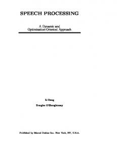
Psychoacoustics (perceptual coding) The processing that takes place in the human auditory system is limited by the perceptual capabilities of the hearing system for which some of the acoustic data is irrelevant. This is of great importance because the digital treatment of signals is still limited by the power of existing computers. In addition, the storage and retrieval of digitally recorded signals could be made more efficient by discarding non-relevant features in the signals. Perceptual acoustic modeling gives us the possibility to judiciously remove some of the speech data that is not perceived by the auditory system and focus on the processing of data is relevant for the human hearing system. The basilar membrane in the internal ear is one of the most important structures for the processing and coding of the acoustic data. The frequency coding represents the equivalent of the spectral analysis which in signal processing is accomplished through the time-domain to frequency-domain transforms. The human auditory system has a frequency-dependent frequency resolution that translates in the requirements to use perceptually weighted frequency scales such as the Mel scale or the Bark scale (see (Harrington & Cassidy, 1999)). The human auditory system also presents a frequency-dependent absolute threshold of hearing as well as a close to logarithmic scale of coding the signals amplitudes (e.g. loudness) which has resulted in the adoption of the decibel scale (Figure 1). Signal components whose amplitudes are below the absolute threshold of hearing can be removed without any loss in the quality of the sound.
80
Sound pressure level (dB)
60
40
20
0
-20 10
100
1000 Frequency (Hz)
Figure 1. The absolute threshold of hearing in quiet for an average listener.
2
10000
100000
DRAFT
The movements of the basilar membrane in the internal ear are collected by the hair cells receptors and the amplitude and frequency information is transmitted to the brain on separate nervous fibers of the auditory nerve (Gold & Morgan, 2000; Møller, 2000). Although we know that the frequency information is transmitted tonotopically to the brain (i.e. nerve fibers are frequency specific), much less is known about how the amplitude information is coded. Modeling the auditory system as a bank of highly overlapping band pass filters of non-uniform bandwidth allows one to account for the psychoacoustics phenomena such as “tone masking” and explain notions such as “critical bands”, all involved in the perception of multiple tone sounds. The “critical bands” notion is well founded on psychoacoustic measurements and knowledge of the hearing organs and implies that the ear can only detect the total sound energy level within a critical band and that the subband frequency details are non-perceptible (Painter & Spanias, 2000). The critical bands are well approximated by the Bark scale and correspond to the human ear frequency resolution and represent the perceptual quantization in frequency (Figure 2). 5000 4500
Critical bandwidth (Hz)
4000 3500 3000 2500 2000 1500 1000 500 0 10
100
1000
10000
100000
Frequency (Hz)
Figure 2. The critical bandwidth increase exponentially with the frequency; The Bark scale models best this behavior.
Frequency masking is a related phenomenon which describes the effect produced by stronger sounds on weaker ones, which are adjacent in the frequency spectrum. For example, when two pure tones close in frequency are presented simultaneously, the stronger one masks the other which may become inaudible (Gold & Morgan, 2000; Painter & Spanias, 2000). These advances made it possible for engineers to devise signal processing algorithms which remove irrelevant features and compress acoustic data beyond the possibilities offered by the general data compression techniques.
1.4
Spectral analysis Spectral analysis or frequency-domain analysis of signals is the main process taking place at the internal ear level. Its most widely used digital signal processing counterpart is the Discrete Fourier Transform (DFT). The Fast Fourier Transform (FFT), a faster implementation of the DFT, is known to
3
DRAFT
1.5
1.5
1
1.0
0.5
0.5
imaginary
imaginary
offer a good approximation for the calculation of the spectrum of signals, providing in the same time improvements in computation time. The DFT and FFT are both particular variants of a more general transform known under the name of z-transform whose name is given by the fact that the computations are performed in the complex numbers plane called the z-plane. Another reason for using spectral analysis is that when dealing with big amounts of digitally recorded sound data, a method of data compression is desirable. As sounds often contain quasi-periodic components, the compression algorithms based on spectral analysis offer the greatest compression ratio and are therefore the most appropriate to use, despite their relatively high computing power demands when compared with other general data compression algorithms. The insights provided by the psychoacoustics research showed that the human auditory system has a non-linear frequency resolution property. Because the FFT is performed at equally distanced points in the frequency plane, many of the resulting higher frequency spectral coefficients are non-relevant from a psychoacoustic point of view. This is so, because the internal ear frequency discrimination is very good at low frequencies and poor at high frequencies, behavior that is modeled by the psychoacoustically correct scales such as the Bark scale. FFT provides a uniform, fixed frequency resolution across the whole spectrum, due to the sampling points which are equally spaced on the unit circle (Figure 3a). This has led to improvements currently known as the Warped Discrete Fourier Transform (WDFT) (Franz, 2002; Makur & Mitra, 2001), a special case of the Non-uniform Discrete Fourier Transform (NDFT), which can model more accurately the human ear frequency-domain processing (Härmä, 1997; Härmä & Laine, 2001). These transforms are using non-uniformly spaced sampling points on the unit circle (Figure 3b). An important consequence of the frequency domain warping is that the energy of the signal is not preserved in the transform which has to be corrected by weighting the sampling points in accord to their density on the z-plane (Pietarila, 2001). In addition, fast implementations such as FFT, for the warped counterparts may not be possible because of the lack of symmetry of the sampling points.
0
0.0
-0.5
-0.5
-1
-1.0
-1.5 -1.5
-1.5 -1.0
-0.5
0.0
0.5
1.0
-1.5
1.5
-1.0
-0.5
0.0
0.5
1.0
1.5
real
real
Figure 3. The z-planes of the FFT and WDFT. a) equally distanced sampling points. b) the non-equally distanced sampling points are more dense in the regions of interest of the frequency spectrum
4
DRAFT
2
Signal processing applications to speech
2.1
Speech synthesis Speaking machines are one of the oldest form of speech application and date from the 1780 (Gold & Morgan, 2000). There is a long history of attempts to speech synthesis which recently concretized in astonishing results (http://www.naturalvoices.att.com/).
A simple model of a speech synthesis system is presented in Figure 4. The two acoustic sources in speech production are the noise and the glottal source. The noise source is always present in the fricative phonemes (e.g. consonants such as /f/, /s/, /ʃ/ /ʃ/), while the glottal source has importance for the voiced phonemes (e.g. the vowels /a/, /a/, /e/, /o/, /u/). The two switches, when both closed, enable the production the phonemes which are both fricative and voiced (e.g. /v/, /z/, /ʒ/ /ʒ/).
Figure 4. A simple model for a speech synthesis system; the glottal source is not a pure tone at the pitch frequency but has a complex spectrum, with many non-zero frequency components (f0, f1, … fn)
2.2
Audio and speech compression The traditional lossless data compression methods (Hufmann, Lempel-Ziv) do not wok well on acoustic data. The audio compression methods are therefore always lossy and are ranging from simple (e.g. silence removers) to more complicated adaptive algorithms (e.g. Adaptive Differential Pulse Code Modulation – ADPCM) which achieve rates of data rate of 16 or 32 kbit/sec by encoding the differences between consecutive signal values rather than the values themselves. Speech compression is usually performed using predictive algorithms such as the Linear Predictive Coding – LPC or Code Excited Linear Predictor (CELP) for data rates of 2.4-4.8 kbit/sec by fitting the signals to a speech model and encoding only the parameters of the model and optionally error terms between the encoded and the original signals (Spanias, 1994). The latest developments in audio compression make use of the insights into the psychoacoustics of the human auditory system and are therefore called perceptual encoders because they remove the non-audible acoustic data by the means of complex signal processing techniques in the frequency domain. The best known compression of this kind is the MPEG-audio compression which achieves data rates of 256 kbit/sec for CD quality audio playback. It is expected that the perceptual compression of speech, whose bandwidth requirements are much smaller than those of CD quality recordings, may achieve much lower bitrates in the condition of a high quality speech recording. This technology is today present in the personal IC (integrated-circuit) recorders. Statistical analysis of speech data1 Frequency-domain speech data is amenable to statistical processing using general multivariate data analysis tools such as principal component analysis. The spectral coefficients need to be normalized on the RMS (i.e. root-mean-square) level of the recordings, in order to account for the differences in energy between the different phonemes.
2.3
1
This is based on work done previously, together with Dr. Tiberiu Spircu, in the Department of Medical Informatics, “Carol Davila” University of Medicine and Pharmacy, Bucharest
5
DRAFT
The map and the confusion matrix of Romanian phonemes 126 spectral coefficients of Romanian language phonemes extracted from recordings made with an ordinary soundcard and microphone, have been fed into a principal component analysis application. Special conditions for studying voiced plosive (e.g. /b/, /d/) and the short (e.g. /g/) voiced consonants have been met, namely to analyze separately the pressure buildup period which is a small component with the frequency of the speaker’s pitch. It is known (Gold & Morgan, 2000) that the spectra of such phonemes exhibit two different patterns, the initial pressure buildup which is very common, followed by the actual acoustic burst with a duration under 20 ms. The principal component analysis yielded a number of three (factors) which "explained" 48% of the variability of the data. The first two principal components have been used to construct a Romanian phoneme map (Figure 5). The "explaining" of the principal components was not an easy task as they are usually associated with many features present in the data. Factor 1 was linked to the 4000-5000 Hz bandwidth, Factor 2 was linked with a particular frequency of around 1330 Hz and Factor 3 was not easy explainable.
Figure 5. A 2-dimensional map of the Romanian phonemes drawn using the first two principal components
From the three principal components, a phoneme distance matrix was obtained (Table 1) by calculating scaled values (i.e. between 0.00 and 1.00) of the relative Euclidean distances between the phoneme spectra, in the 3-dimensional space of principal components. The matrix may help with explaining some of the confusions that are found in spoken Romanian language. The maximal value in the table (i.e. 1.00) was found between the phonemes /e/ and /s/, that is between a vowel and the fricative consonant with high frequency components in its spectrum. This can be explained by the simple observation that the spectra of the two phonemes are complementary, i.e. the /e/ is a vowel (i.e. voiced phoneme) with a rich low frequency spectrum while the /s/ is a non-voiced fricative with a rich high-frequency spectrum. This complementarity yields the increased value of the Euclidean distance.
6
DRAFT
The minimal values in the table (i.e. 0.00-0.01) are between the spectra of pressure buildup of the plosive (i.e. /b/, /d/, /g/ and voiced fricative consonants /ɣ/. Other observations that can be derived from the distance matrix are the very similar phoneme pairs such as /m/– /m/–/n/ (main difference in Factor 3), /u/– /u/–/l/ (main difference in Factor 1) and /o/– /o/–/b2/ (main difference in Factor 1), where /b2/ represents the acoustic burst of the phoneme /b/. Other possible confusion pairs with small relative distances are: •
/m/– /m/–/b2/,
•
/v/– /v/–/r/,
differences in Factors 1 and 2;
•
/l/– /l/–/n/,
difference in Factor 3;
•
/u/– /u/–/n/,
•
/ɨ/– ɨ/–/l/,
•
/ɨ/– ɨ/–/u/,
•
/p/– /p/–/b2/,
•
/m/– /m/–/p/,
•
/ɣ/ ɣ/– –/ʒ/,
differences in Factors 1 and 2;
•
/l/– /l/–/m/,
difference in Factor 3;
•
/o/– /o/–/m/,
differences in Factors 1 and 2;
•
/ə/– ə/–/d2/,
difference in Factor 1.
main difference in Factor 2;
difference in Factor 1;
difference in Factor 2; differences in Factors 1 and 2. main difference in Factor 1;
differences in Factors 1 and 2;
The study of formant transitions When a speaker is making a transition from a vowel to another during the pronunciation of a word, the natural way to do this is by performing a format transition from the first vowel to the second vowel. So, between the two actual phonemes there will be a short transition zone, which sometimes could resemble another phoneme. This may be of importance to speech intelligibility because it provides a clear indication of the direction of the frequency spectrum shifting which could overcome a possible faulty audition of one of the two phonemes. For example, the transition from the /i/ to /a/ (Figure 6 - left) contains a short zone, momentarily resembling the phoneme /e/ (Figure 6 - right). The spectral analysis indicates that there is no pure /ia/ utterance but rather variants of /iea/ in which the /e/ is quite short, therefore difficult to perceive. This idea is also suggested by the way some people feel natural to pronounce the interjection /ia/ as /iea/ and record in writing this particular utterance as “yeah” which describes more accurately the acoustic phenomenon.
7
DRAFT
/i/ transition /a/
Figure 6. The spectrograms of /ia/ (left) and /e/ (right)
After preprocessing, the short term spectral data of the recorded /ia/ was regarded as successive points in a multidimensional space, traveling from a starting point represented by the beginning of the /i/, to the end point, the silence after the phoneme /a/. It is important to note that, in this particular experiment, the beginning of the /i/ was represented by the silence before pronunciation and the end of the phoneme /a/ by the silence after pronunciation. Therefore, the evolution in time of the acoustic patterns formed a loop with a common start-end point. The three principal components extracted by the factorial analysis from the given acoustic parameters set, made possible graphical representation of the pronunciation evolution. The representation of the utterance /ia/ in the plane of the first two principal components looks like Figure 7. A separately recorded phoneme /e/ was also represented.
Figure 7. The graphic representation of the utterance /ia/ in the plane of the first two principal components
8
DRAFT
Figure 8. The graphic representation of the utterance /ia/ in the plane of the first and third principal components
As one may observe, the pronunciation evolution overlaps partially the pattern space of the phoneme especially during the transition phase, which has been labeled "IA". The phenomenon is better depicted in the plane of the factors 1 and 3 (Figure 8). The initial observation that when pronouncing /ia/ one actually pronounces a variant of /iea/, is confirmed experimentally.
/e/,
2.4
Analysis of speech data using artificial neural networks Artificial neural network emerged in the last 20 years as powerful, adaptive data processing models for pattern classification and feature extraction (Rumelhart, Hinton, & Williams, 1986). They come in various configurations and their main characteristic is the capability of learning from examples, creating new information processing functions such as specific feature detectors. It is stated (Kohonen, 2001) that only neural networks are able to create higher abstractions (symbolisms) from raw data, completely automatically and this is what makes them intelligent. A well known speech processing application of neural networks employed self organizing maps (Kohonen, 2001). Finish phoneme maps obtained demonstrated how systems are able to automatically cluster the phonemes based on the similarity of their spectral coefficients of the speech signals and help with the visualization of the trajectory of utterances, analysis of speech articulation, and speech pathology analysis (Figure 9) (Kangas, 1994).
9
DRAFT
Figure 9. A self organizing map computed from Finish speech samples from 15 men. The trajectory produced by the utterance /sa:ri/ is shown by the poly-line starting in /s/ and ending in /i/ (from (Kangas, 1994))
3
Outlook
Signal processing applications for speech processing and the psychoacoustic modeling of the human hearing system are very well advanced. However, the higher level processing of speech, i.e. the cognitive phenomena and information processing taking place in the brain are still separated from sound analysis. The coupling between speech and sound processing with the higher cognitive faculties such as language processing, must therefore be pursued as they will surely prove fruitful. It is commonly accepted that human speech recognition is based on a continuum of information processing operations which couple sound and speech processing with natural language understanding and that the exceptionally low signal to noise ratios of speech that humans are able to tolerate comes mainly from the natural language processing abilities. The idea of a unifying model for speech and natural language processing similar to Fletcher’s recognition chain discussed in (Allen, 1995), although potentially unfeasible with the computing power available today, is therefore a very desirable direction of research.
10
DRAFT IPA Description p b1 b2 t d1 d2 c g1
g2 m n r f v
Voiceless bilabial stop Voiced bilabial stop Voiceless alveolar stop Voiced alveolar stop Voiceless palatal stop Voiced velar stop Bilabial nasal Alveolar nasal Alveolar trill Voiceless labiodental fricative Voiced labiodental fricative
p
Code 101 101 0.09 102 0.05 103 0.16 0.09 104 0.09 107 0.60 0.08 110 0.52 114 0.05 116 0.06 122 0.16 128 0.54 129 0.21
b1b1 -b2
102
0.10 0.25 0.01 0.18 0.64 0.02 0.59 0.06 0.07 0.22 0.62 0.27
t
103
d1d1-d2
104
c
107
g1g1-g2
110
m
n
r
f
302 304 307 308 317 322
301 0.33 0.51 0.27 0.23 0.20 0.26
i
0.17 0.10 0.09 0.58 0.08 0.50 0.04 0.06 0.15 0.55 0.19
0.25 0.08 0.51 0.24 0.37 0.20 0.21 0.12 0.39 0.15
e
0.18 0.64 0.01 0.59 0.05 0.06 0.22 0.63 0.27
a
0.57 0.16 0.45 0.12 0.12 0.14 0.48 0.18
o
0.64 0.27 0.62 0.64 0.43 0.40 0.38
u
0.58 0.04 0.05 0.21 0.62 0.26
ɨ
0.55 0.56 0.37 0.20 0.33
v
s
z
ʃ
ʒ
e
a
o
u
ɨ
ə
0.69 0.55 0.53 0.49 0.50
z
Voiced alveolar fricative Voiceless postalveolar fricative Voiced postalveolar fricative Voiceless velar stop Voiced velar fricative Voiceless uvular fricative Alveolar lateral approximant Cardinal vowel 1: close front unrounded Cardinal vowel 2: close-mid front unrounded Cardinal vowel 4: open front unrounded Cardinal vowel 7: close-mid back rounded Cardinal vowel 8: close back rounded Close central unrounded vowel Mid central vowel
133 134 135 140
ʃ ʒ k ɣ1
ɣ2 χ l i e a o u ɨ ə
141 142 155 301 302 304 307 308 317 322
0.40 0.44 0.41 0.53 0.25 0.45 0.21 0.19 0.25 0.46 0.25 0.17 0.21 0.17 0.11
0.29 0.63 0.48 0.56 0.00 0.50 0.26 0.10 0.32 0.63 0.35 0.11 0.11 0.14 0.18
0.39 0.50 0.44 0.55 0.18 0.47 0.22 0.10 0.22 0.48 0.29 0.09 0.12 0.08 0.05
0.59 0.73 0.72 0.86 0.64 0.77 0.38 0.64 0.77 0.88 0.29 0.59 0.66 0.63 0.54
Table 1. Relative distances between Romanian language phonemes.
11
0.30 0.62 0.48 0.56 0.01 0.50 0.25 0.09 0.31 0.62 0.34 0.09 0.09 0.13 0.17
0.64 0.53 0.62 0.77 0.59 0.68 0.37 0.55 0.59 0.63 0.30 0.51 0.56 0.53 0.44
0.32 0.60 0.48 0.57 0.05 0.51 0.23 0.05 0.28 0.58 0.32 0.05 0.06 0.09 0.13
0.34 0.60 0.48 0.57 0.06 0.51 0.25 0.04 0.26 0.57 0.34 0.06 0.04 0.08 0.13
0.33 0.54 0.46 0.59 0.22 0.50 0.09 0.21 0.36 0.58 0.15 0.16 0.22 0.20 0.12
0.64 0.36 0.50 0.64 0.63 0.55 0.47 0.59 0.58 0.59 0.40 0.56 0.60 0.56 0.49
χ
l
142 155
0.30 0.36 0.06 0.35 0.06 0.04 0.26 0.07 0.12 0.09 Scale 0.00 0.01 0.02 0.05 0.06 0.10 0.11 0.20
132 0.52 0.49 0.56 0.59 0.51 0.59 0.73 0.52 0.79 0.54 0.56 0.54 0.74 0.55 0.34 0.59 0.48 0.58 0.09 0.52 0.20 0.07 0.28 0.57 0.28 0.02 0.08 0.08 0.08
141
0.02 0.19 0.20 0.59 0.60 0.43 0.24 0.25 0.04 0.39
Voiceless alveolar fricative
0.28 0.62 0.47 0.55 0.01 0.49 0.26 0.10 0.32 0.63 0.35 0.11 0.11 0.14 0.18
ɣ1ɣ1-ɣ2
302 304 307 308 317
s
0.32 0.55 0.43 0.53 0.09 0.46 0.22 0.07 0.26 0.56 0.37 0.08 0.11 0.11 0.13
k
114 116 122 128 129 132 133 134 135 140
0.35 0.53 0.47 0.60 0.27 0.51 0.08 0.26 0.40 0.60 0.11 0.21 0.27 0.25 0.17
0.21 0.40 0.23 0.72 0.42 0.46 0.51 0.43 0.55 0.59 0.71 1.00 0.58 0.58 0.60 0.62 0.61
0.66 0.42 0.50 0.29 0.44 0.33 0.38 0.55 0.84 0.38 0.36 0.39 0.41 0.40
0.41 0.70 0.71 1.00 0.31 0.39 0.63 0.34 0.62 0.58 0.46 0.47 0.61 0.59 0.60 0.56 0.54
0.14 0.48 0.05 0.53 0.48 0.46 0.65 0.55 0.50 0.50 0.49 0.49
0.56 0.09 0.66 0.57 0.53 0.72 0.68 0.59 0.59 0.58 0.60
0.51 0.26 0.10 0.32 0.63 0.35 0.10 0.11 0.14 0.18
0.57 0.51 0.48 0.67 0.59 0.53 0.53 0.52 0.52
0.27 0.44 0.66 0.09 0.21 0.28 0.27 0.19
0.23 0.53 0.35 0.06 0.02 0.04 0.11
DRAFT
References Allen, J. B. (1995). How do humans process and recognize speech? In R. P. Ramachandran & R. J. Mammone (Eds.), Modern methods of speech processing (pp. xvii, 470). Boston: Kluwer Academic Publishers. Franz, S. M., S.K.; Schmidt, J.C.; Doblinger, G. (2002). Warped discrete Fourier transform: a new concept in digital signal processing. Paper presented at the Acoustics, Speech, and Signal Processing, 2002 IEEE International Conference on. Gold, B., & Morgan, N. (2000). Speech and audio signal processing : processing and perception of speech and music. New York: John Wiley. Härmä, A. (1997). Perceptual aspects and warped techniques in audio coding. Unpublished Master of Science, Helsinki University of Technology, Helsinki. Härmä, A., & Laine, U. K. (2001). A Comparison of Warped and Conventional Linear Predictive Coding. IEEE TRANSACTIONS ON SPEECH AND AUDIO PROCESSING, 9(5), 579-588. Harrington, J., & Cassidy, S. (1999). Techniques in speech acoustics. Dordrecht Boston: Kluwer Academic Publishers. Kangas, J. (1994). On the Analysis of Pattern Sequences by Self-Organizing Maps. Unpublished PhD, Helsinki University of Technology, Espoo, Finland. Kohonen, T. (2001). Self-Organizing Maps ( 3rd ed. ed. Vol. 30). Berlin Heidelberg New York: Springer-Verlag. Makur, A., & Mitra, S. K. (2001). Warped Discrete-Fourier Transform: Theory and Applications. IEEE TRANSACTIONS ON CIRCUITS AND SYSTEMS, 48(9), 1086-1093. Møller, A. R. (2000). Hearing : its physiology and pathophysiology. San Diego: Academic Press. Painter, T., & Spanias, A. (2000). Perceptual coding of digital audio. Proceedings of the IEEE, 88(4), 451-515. Pietarila, P. (2001). A Frequency-Warped Front-End for a Subband Audio Codec. Unpublished Diploma, University of Oulu, Oulu. Rumelhart, D. E., Hinton, G. E., & Williams, R. J. (1986). Parallel Distributed Processing ( Vol. 1-2): MIT Press. Spanias, A. (1994). Speech coding: A tutorial review. Proceedings of the IEEE, 82(10), 1541-1582.
12