To make a clinical decision on someone, one ... more assumptions may have to
be made about the data. Categorizing .... It is easy to include more information in
a box-whisker plot. ...... Given a sample of disease free subjects, an alternative.
Biostatistics Made Easy: A Guide for Air Force Public Health Professionals Contents 1.
Data display and summary
2.
Mean and standard deviation
3.
Populations and samples
4.
Statements of probability and confidence intervals
5.
Differences between means: type I and type II errors and power
6.
Differences between percentages and paired alternatives
7.
The t-tests
8.
The chi-squared tests
9.
Exact probability test
10. Rank score tests 11. Correlation and regression 12. Survival analysis 13. Study design and choosing a statistical test Appendix A - Probabilities related to multiples of standard deviations for a Normal distribution Appendix B - Distribution of t (two tailed) Appendix C - Distribution of µ Appendix D - Wilcoxon test on paired samples: 5% and 1% levels of P Appendix E - Mann-Whitney test on unpaired samples: 5% and 1% levels of P Appendix F - Random Numbers Glossary of Statistical Terms
Adapted and Modified from: T.D.V. Swinscow, Statistics at Square One, 9th Edition, Revised by M.J. Campbell, University of Southampton, UK
Chapter 1.
Data Display and Summary Types of data The first step, before any calculations or plotting of data, is to decide what type of data one is dealing with. There are a number of typologies, but one that has proven useful is given in Table 1.1. The basic distinction is between quantitative variables (for which one asks "how much?") and categorical variables (for which one asks "what type?"). Quantitative variables can be continuous or discrete. Continuous variables, such as height, can in theory take any value within a given range. Examples of discrete variables are: number of children in a family, number of attacks of asthma per week. Categorical variables are either nominal (unordered) or ordinal (ordered). Examples of nominal variables are male/female, alive/dead, blood group O, A, B, AB. For nominal variables with more than two categories the order does not matter. For example, one cannot say that people in blood group B lie between those in A and those in AB. Sometimes, however, people can provide ordered responses, such as grade of breast cancer, or they can "agree", "neither agree nor disagree", or "disagree" with some statement. In this case the order does matter and it is usually important to account for it. Table 1.1 Examples of types of data Quantitative Continuous
Discrete
Blood pressure, height, weight, age
Number of children Number of attacks of asthma per week Categorical
Ordinal (Ordered categories)
Nominal (Unordered categories)
Grade of breast cancer Better, same, worse Disagree, neutral, agree
Sex (male/female) Alive or dead Blood group O, A, B, AB
Variables shown at the left of Table 1.1 can be converted to ones further to the right by using "cut off points". For example, blood pressure can be turned into a nominal variable by defining "hypertension" as a diastolic blood pressure greater than 90 mmHg, and "normotension" as blood pressure less than or equal to 90 mmHg. Height (continuous) can be converted into "short", "average" or "tall" (ordinal). In general it is easier to summarize categorical variables, and so quantitative variables are often converted to categorical ones for descriptive purposes. To make a clinical decision on someone, one does not need to know the exact serum potassium level (continuous) but whether it is within the normal range (nominal). It may be easier to think of the proportion of the population who are hypertensive than the distribution of blood pressure. However, categorizing a continuous variable reduces the amount of information available and statistical tests will in general be more sensitive - that is they will have more power (see Chapter 5 for a definition of power) for a continuous variable than the corresponding nominal one, although more assumptions may have to be made about the data. Categorizing data is therefore useful for summarizing results, but not for statistical analysis. It is often not appreciated that the choice of appropriate cut off points can be difficult, and different choices can lead to different conclusions about a set of data. These definitions of types of data are not unique, nor are they mutually exclusive, and are given as an aid to help an investigator decide how to display and analyze data. One should not debate long over the typology of a particular variable!
Stem and leaf plots Before any statistical calculation, even the simplest, is performed the data should be tabulated or plotted. If they are quantitative and relatively few, say up to about 30, they are conveniently written down in order of size. For example, a pediatric registrar in a district general hospital is investigating the amount of lead in the urine of children from a nearby housing estate. In a particular street there are 15 children whose ages range from 1 year to under 16, and in a preliminary study the registrar has found the following amounts of urinary lead ( ), given in Table 1.2 what is called an array:
Table 1.2 Urinary concentration of lead in 15 children from housing area X ( ) 0.6, 2.6, 0.1, 1.1, 0.4, 2.0, 0.8, 1.3, 1.2, 1.5, 3.2, 1.7, 1.9, 1.9, 2.2
A simple way to order, and also to display, the data is to use a stem and leaf plot. To do this we need to abbreviate the observations to two significant digits. In the case of the urinary concentration data, the digit to the left of the decimal point is the "stem" and the digit to the right the "leaf".
We first write the stems in order down the page. We then work along the data set, writing the leaves down "as they come". Thus, for the first data point, we write a 6 opposite the 0 stem. These are as given in Figure 1.1.
Figure 1.1 Stem and leaf "as they come" Stem
Leaf
0
6
1
4
8
1
1
3
2
5
2
6
0
2
3
2
7
9
9
We then order the leaves, as in Figure 1.2
Figure 1.2 Ordered stem and leaf plot Stem
Leaf
0
1
4
6
8
1
1
2
3
5
2
0
2
6
3
2
7
9
9
The advantage of first setting the figures out in order of size and not simply feeding them straight from notes into a calculator (for example, to find their mean) is that the relation of each to the next can be looked at. Is there a steady progression, a noteworthy hump, a considerable gap? Simple inspection can disclose irregularities. Furthermore, a glance at the figures gives information on their range. The smallest value is 0.1 and the largest is 3.2 .
Median To find the median (or mid point) we need to identify the point which has the property that half the data are greater than it, and half the data are less than it. For 15 points, the mid point is clearly the eighth largest, so that seven points are less than the median, and seven points
are greater than it. This is easily obtained from Figure 1.2 by counting the eighth leaf, which is 1.5 . To find the median for an even number of points, the procedure is as follows. Suppose the pediatric registrar obtained a further set of 16 urinary lead concentrations from children living in the countryside in the same county as the hospital? (Table 1.3)
Table 1.3 Urinary concentration of lead in 16 rural children ( ) 0.2, 0.3, 0.6, 0.7, 0.8, 1.5, 1.7, 1.8, 1.9, 1.9, 2.0, 2.0, 2.1, 2.8, 3.1, 3.4 To obtain the median we average the eighth and ninth points (1.8 and 1.9) to get 1.85 . In general, if n is even, we average the n/2nd largest and the n/2 + 1st largest observations. The main advantage of using the median as a measure of location is that it is "robust" to outliers. For example, if we had accidentally written 34 rather than 3.4 in Table 1.2 , the median would still have been 1.85. One disadvantage is that it is tedious to order a large number of observations by hand (there is usually no "median" button on a calculator).
Measures of variation It is informative to have some measure of the variation of observations about the median. The range is very susceptible to what are known as outliers, points well outside the main body of the data. For example, if we had made the mistake of writing 34 instead 3.4 in Table which is clearly misleading. 1.2, then the range would be written as 0.1 to 34 A more robust approach is to divide the distribution of the data into four, and find the points below which are 25%, 50% and 75% of the distribution. These are known as quartiles, and the median is the second quartile. The variation of the data can be summarized in the interquartile range, the distance between the first and third quartile. With small data sets and if the sample size is not divisible by four, it may not be possible to divide the data set into exact quarters, and there are a variety of proposed methods to estimate the quartiles. A simple, consistent method is to find the points midway between each end of the range and the median. Thus, from Figure 1.2, there are eight points between and including the smallest, 0.1, and the median, 1.5. Thus the mid point lies between 0.8 and 1.1, or 0.95. This is the first quartile. Similarly the third quartile is mid-way between 1.9 and 2.0, or 1.95. Thus, the . interquartile range is 0.95 to 1.95
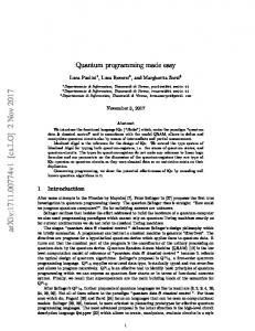
Data display The simplest way to show data is a dot plot. Figure 1.3 shows the data from Tables 1.2 and 1.3 and together with the median for each set.
Figure 1.3 Dot plot of urinary lead concentrations for urban and rural children.
Sometimes the points in separate plots may be linked in some way, for example the data in Table 1.2 and Table 1.3 may result from a matched case control study (see Chapter 13 for a description of this type of study) in which individuals from the countryside were matched by age and sex with individuals from the town. If possible the links should be maintained in the display, for example by joining matching individuals in Figure 1.3. This can lead to a more sensitive way of examining the data. When the data sets are large, plotting individual points can be cumbersome. An alternative is a box-whisker plot. The box is marked by the first and third quartile, and the whiskers extend to the range. The median is also marked in the box, as shown in Figure 1.4
Figure 1.4 Box-whisker plot of data from Figure 1.3
It is easy to include more information in a box-whisker plot. One method, which is implemented in some computer programs, is to extend the whiskers only to points that are 1.5 times the interquartile range below the first quartile or above the third quartile, and to show remaining points as dots, so that the number of outlying points is shown.
Histograms Suppose the pediatric registrar referred to earlier extends the urban study to the entire estate in which the children live. He obtains figures for the urinary lead concentration in 140 children aged over 1 year and under 16. We can display these data as a grouped frequency table (Table 1.4). Table 1.4 Lead concentration in 140 children Lead concentration ( )
Number of children
0-
2
0.4-
7
0.8-
10
1.2-
16
1.6-
23
2.0-
28
2.4
19
2.8-
16
3.2-
11
3.6-
7
2.4
19
2.8-
16
3.2-
11
3.6-
7
4.0-
1
4.4Total
140
Figure 1.5 Histogram of data from Table 1.4
Bar charts Suppose, of the 140 children, 20 lived in owner occupied houses, 70 lived in council houses and 50 lived in private rented accommodation. Figures from the census suggest that for this
age group, throughout the county, 50% live in owner occupied houses, 30% in council houses, and 20% in private rented accommodation. Type of accommodation is a categorical variable, which can be displayed in a bar chart. We first express our data as percentages: 14% owner occupied, 50% council house, 36% private rented. We then display the data as a bar chart. The sample size should always be given (Figure 1.6).
Figure 1.6 Bar chart of housing data for 140 children and comparable census data
.
Common questions How many groups should I have for a histogram? In general one should choose enough groups to show the shape of a distribution, but not too many to lose the shape in the noise. It is partly aesthetic judgment but, in general, between 5 and 15, depending on the sample size, gives a reasonable picture. Try to keep the intervals (known also as "bin widths") equal. With equal intervals the height of the bars and the area of the bars are both proportional to the number of subjects in the group. With unequal intervals this link is lost, and interpretation of the figure can be difficult.
What is the distinction between a histogram and a bar chart? Alas, with modern graphics programs the distinction is often lost. A histogram shows the distribution of a continuous variable and, since the variable is continuous, there should be no
gaps between the bars. A bar chart shows the distribution of a discrete variable or a categorical one, and so will have spaces between the bars. It is a mistake to use a bar chart to display a summary statistic such as a mean, particularly when it is accompanied by some measure of variation to produce a "dynamite plunger plot"(1). It is better to use a box-whisker plot.
What is the best way to display data? The general principle should be, as far as possible, to show the original data and to try not to obscure the design of a study in the display. Within the constraints of legibility show as much information as possible. If data points are matched or from the same patients link them with lines. (2) When displaying the relationship between two quantitative variables, use a scatter plot (Chapter 11) in preference to categorizing one or both of the variables.
References 1. Campbell M J. How to present numerical results. In: How to do it: 2. London: BMJ Publishing, 1995:77-83. 2. Matthews J N S, Altman D G, Campbell M J, Royston J P. Analysis of serial measurements in medical research. BMJ1990; 300:230-5.
Exercises Exercise 1.1 From the 140 children whose urinary concentration of lead were investigated 40 were chosen who were aged at least 1 year but under 5 years. The following concentrations of copper (in ) were found. 0.70, 0.45, 0.72, 0.30, 1.16, 0.69, 0.83, 0.74, 1.24, 0.77, 0.65, 0.76, 0.42, 0.94, 0.36, 0.98, 0.64, 0.90, 0.63, 0.55, 0.78, 0.10, 0.52, 0.42, 0.58, 0.62, 1.12, 0.86, 0.74, 1.04, 0.65, 0.66, 0.81, 0.48, 0.85, 0.75, 0.73, 0.50, 0.34, 0.88 Find the median, range, and quartiles.
Chapter 2.
Mean and Standard Deviation The median is known as a measure of location; that is, it tells us where the data are. As stated in, we do not need to know all the exact values to calculate the median; if we made the smallest value even smaller or the largest value even larger, it would not change the value of the median. Thus the median does not use all the information in the data and so it can be shown to be less efficient than the mean or average, which does use all values of the data. To calculate the mean we add up the observed values and divide by the number of them. The total of the values obtained in Table 1.1 was 22.5 , which was divided by their number, 15, to give a mean of 1.5 . This familiar process is conveniently expressed by the following symbols:
(pronounced "x bar") signifies the mean; x is each of the values of urinary lead; n is the number of these values; and , the Greek capital sigma (our "S") denotes "sum of". A major disadvantage of the mean is that it is sensitive to outlying points. For example, replacing 2.2 by , whereas the median will be unchanged. 22 in Table 1.1 increases the mean to 2.82 As well as measures of location we need measures of how variable the data are. We met two of these measures, the range and interquartile range, in Chapter 1. The range is an important measurement, for figures at the top and bottom of it denote the findings furthest removed from the generality. However, they do not give much indication of the spread of observations about the mean. This is where the standard deviation (SD) comes in. The theoretical basis of the standard deviation is complex and need not trouble the ordinary user. We will discuss Sampling and Populations in Chapter 3. A practical point to note here is that, when the population from which the data arise have a distribution that is approximately "Normal" (or Gaussian), then the standard deviation provides a useful basis for interpreting the data in terms of probability.
The Normal distribution is represented by a family of curves defined uniquely by two parameters, which are the mean and the standard deviation of the population. The curves are always symmetrically bell shaped, but the extent to which the bell is compressed or flattened out depends on the standard deviation of the population. However, the mere fact that a curve is bell shaped does not mean that it represents a Normal distribution, because other distributions may have a similar sort of shape. Many biological characteristics conform to a Normal distribution closely enough for it to be commonly used - for example, heights of adult men and women, blood pressures in a healthy population, random errors in many types of laboratory measurements and biochemical data. Figure 2.1 shows a Normal curve calculated from the diastolic blood pressures of 500 men, mean 82 mmHg, standard deviation 10 mmHg. The ranges representing , , and about the mean are marked. A more extensive set of values is given in Table A (Appendix)
Figure 2.1 Normal curve calculated from diastolic blood pressures of 500 men, mean 82 mmHg, standard deviation 10 mmHg.
The reason why the standard deviation is such a useful measure of the scatter of the observations is this: if the observations follow a Normal distribution, a range covered by one standard deviation above the mean and one standard deviation below it (
) includes
about 68% of the observations; a range of two standard deviations above and two below ( ) about 95% of the observations; and of three standard deviations above and three below ( ) about 99.7% of the observations. Consequently, if we know the mean and standard deviation of a set of observations, we can obtain some useful information by simple arithmetic. By putting one, two, or three standard deviations above and below the mean we can estimate the ranges that would be expected to include about 68%, 95%, and 99.7% of the observations.
Standard Deviation from Ungrouped Data The standard deviation is a summary measure of the differences of each observation from the mean. If the differences themselves were added up, the positive would exactly balance the negative and so their sum would be zero. Consequently the squares of the differences are added. The sum of the squares is then divided by the number of observations minus one to give the mean of the squares, and the square root is taken to bring the measurements back to the units we started with. (The division by the number of observations minus one instead of the number of observations itself to obtain the mean square is because "degrees of freedom" must be used. In these circumstances they are one less than the total. The theoretical justification for this need not trouble the user in practice.) To gain an intuitive feel for degrees of freedom, consider choosing a chocolate from a box of n chocolates. Every time we come to choose a chocolate we have a choice, until we come to the last one (normally one with a nut in it!), and then we have no choice. Thus we have n-1 choices, or "degrees of freedom". The calculation of the variance is illustrated in Table 2.1 with the 15 readings in the preliminary study of urinary lead concentrations (Table 1.2). The readings are set out in column (1). In column (2) the difference between each reading and the mean is recorded. The sum of the differences is 0. In column (3) the differences are squared, and the sum of those squares is given at the bottom of the column.
Table 2.1 Calculation of standard deviation (1) Lead concentration
(2) Differences from mean
(3) Differences squared
(4) Observations in column (1) ß squared
0.1
-1.4
1.96
0.01
0.4
-1.1
1.21
0.16
Total n= 15,
0.6
-0.9
0.81
0.36
0.8
-0.7
0.49
0.64
1.1
-0.4
0.16
1.21
1.2
-0.3
0.09
1.44
1.3
-0.2
0.04
1.69
1.5
0
0
2.25
1.7
0.2
0.04
2.89
1.9
0.4
0.16
3.61
1.9
0.4
0.16
3.61
2.0
0.5
0.25
4.00
2.2
0.7
0.49
4.84
2.6
1.1
1.21
6.76
3.2
1.7
2.89
10.24
22.5
0
9.96
43.71
= l.5
The sum of the squares of the differences (or deviations) from the mean, 9.96, is now divided by the total number of observation minus one, to give the variance. Thus,
In this case we find:
Finally, the square root of the variance provides the standard deviation:
from which we get
This procedure illustrates the structure of the standard deviation, in particular that the two extreme values 0.1 and 3.2 contribute most to the sum of the differences squared.
Calculator procedure Most inexpensive calculators have procedures that enable one to calculate the mean and standard deviations directly, using the "SD" mode. For example, on modern Casio® calculators one presses SHIFT and '.' and a little "SD" symbol should appear on the display. On earlier Casio®'s one presses INV and MODE, whereas on a Sharp® 2nd F and Stat should be used. The data are stored via the M+ button. Thus, having set the calculator into the "SD" or "Stat" mode, from Table 2.1 we enter 0.1 M+, 0.4 M+, etc. When all the data are entered, we can check that the correct number of observations have been included by Shift and n and "15" should be displayed. The mean is displayed by Shift and and
and the standard deviation by Shift
. Avoid pressing Shift and AC between these operations as this clears the statistical
memory. There is another button (
) on many calculators. This uses the divisor n rather than
n - 1 in the calculation of the standard deviation. On a Sharp calculator
is denoted
,
whereas is denoted s. These are the "population" values, and are derived assuming that an entire population is available or that interest focuses solely on the data in hand, and the results are not going to be generalized (see Chapter 3 for details of Samples and Populations). As this situation very rarely arises, should be used and ignored, although even for moderate sample sizes the difference is going to be small. Remember to return to normal mode before resuming calculations because many of the usual functions are not available in "Stat" mode. On a modern Casio® this is Shift 0. On earlier Casio®'s and on Sharps® one repeats the sequence that call up the "Stat" mode. Some calculators stay in "Stat" mode even when switched off. Mullee (1) provides advice on choosing and using a calculator. The calculator formulas use the relationship
The right hand expression can be easily memorized by the expression mean of the squares minus the mean square". The sample variance
is obtained from
The above equation can be seen to be true in Table 2.1, where the sum of the square of the observations,
, is given as 43.7l. We thus obtain
the same value given for the total in column (3). Care should be taken because this formula involves subtracting two large numbers to get a small one, and can lead to incorrect results if the numbers are very large. For example, try finding the standard deviation of 100,001, 100,002, 100,003 on a calculator. The correct answer is 1, but many calculators will give 0 because of rounding error. The solution is to subtract a large number from each of the observations (say 100,000) and calculate the standard deviation on the remainders, namely 1, 2, and 3. Standard Deviation from Grouped Data We can also calculate a standard deviation for discrete quantitative variables. For example, in addition to studying the lead concentration in the urine of 140 children, the pediatrician asked how often each of them had been examined by a doctor during the year. After collecting the information he tabulated the data shown in Table 2.2 columns (1) and (2). The mean is calculated by multiplying column (1) by column (2), adding the products, and dividing by the total number of observations. Table 2.2 Calculation of the standard deviation from qualitative discrete data (1) Number of visits to or by doctor
(2) Number of children
(3) Col (2) x Col (1)
(4) Col (1) squared
(5) Col (2) x Col (4)
0
2
0
0
0
1
8
8
1
8
2
27
54
4
108
3
45
135
9
405
4
38
152
16
608
5
15
75
25
375
6
4
24
36
144
7
1
7
49
49
Total
140
455
Mean number of visits = 455/140 = 3.25.
1697
As we did for continuous data, to calculate the standard deviation we square each of the observations in turn. In this case the observation is the number of visits, but because we have several children in each class, shown in column (2), each squared number (column (4)), must be multiplied by the number of children. The sum of squares is given at the foot of column (5), namely 1697. We then use the calculator formula to find the variance:
and
Note that although the number of visits is not Normally distributed, the distribution is reasonably symmetrical about the mean. The approximate 95% range is given by
This excludes two children with no visits and six children with six or more visits. Thus there are eight of 140 = 5.7% outside the theoretical 95% range. Note that it is common for discrete quantitative variables to have what is known as skewed distributions, that is they are not symmetrical. One clue to lack of symmetry from derived statistics is when the mean and the median differ considerably. Another is when the standard deviation is of the same order of magnitude as the mean, but the observations must be nonnegative. Sometimes a transformation will convert a skewed distribution into a symmetrical one. When the data are counts, such as number of visits to a doctor, often the square root transformation will help, and if there are no zero or negative values a logarithmic transformation will render the distribution more symmetrical.
Data Transformation An anesthetist measures the pain of a procedure using a 100mm visual analogue scale on seven patients. The results are given in Table 2.3, together with the loge transformation (the ln button on a calculator).
Table 2.3 Results from pain score on seven patients (mm) Original scale:
1, 1, 2, 3, 3, 6, 56
Loge scale:
0, 0, 0.69, 1.10, 1.10, 1.79, 4.03
The data are plotted in Figure 2.2, which shows that the outlier does not appear so extreme in the logged data. The mean and median are 10.29 and 2, respectively, for the original data, with a standard deviation of 20.22. Where the mean is bigger than the median, the distribution is positively skewed. For the logged data the mean and median are 1.24 and 1.10 respectively, indicating that the logged data have a more symmetrical distribution. Thus it would be better to analyze the logged transformed data in statistical tests than using the original scale.
Figure 2.2 Dot plots of original and logged data from pain scores
. In reporting these results, the median of the raw data would be given, but it should be explained that the statistical test was carried out on the transformed data. Note that the median of the logged data is the same as the log of the median of the raw data - however, this is not true for the mean. The mean of the logged data is not necessarily equal to the log of the mean of the raw data. The antilog (exp or on a calculator) of the mean of the logged data is known as the geometric mean, and is often a better summary statistic than the mean for data from positively skewed distributions. For these data the geometric mean in 3.45 mm.
Between (inter-)subjects and Within (intra-)subjects Standard Deviation If repeated measurements are made of, say, blood pressure on an individual, these measurements are likely to vary. This is within subject, or intra-subject, variability and we can calculate a standard deviation of these observations. If the observations are close together in time, this standard deviation is often described as the measurement error. Measurements made on different subjects vary according to between subject, or inter-subject, variability. If many observations were made on each individual, and the average taken, then we can assume that the intra-subject variability has been averaged out and the variation in the average values is due solely to the inter-subject variability. Single observations on individuals clearly contain a mixture of inter-subject and intra-subject variation. The coefficient of variation (CV%) is the intra-subject standard deviation divided by the mean, expressed as a percentage. It is often quoted as a measure of repeatability for biochemical assays, when an assay is carried out on several occasions on the same sample. It has the advantage of being independent of the units of measurement, but also numerous theoretical disadvantages. It is usually nonsensical to use the coefficient of variation as a measure of between subject variability.
Common questions When should I use the mean and when should I use the median to describe my data? It is a commonly held misapprehension that for Normally distributed data one uses the mean, and for non-Normally distributed data one uses the median. Unfortunately, this is not so: if the data are Normally distributed the mean and the median will be close; if the data are not Normally distributed then both the mean and the median may give useful information. Consider a variable that takes the value 1 for males and 0 for females. This is clearly not Normally distributed. However, the mean gives the proportion of males in the group, whereas the median merely tells us which group contained more than 50% of the people. Similarly, the mean from ordered categorical variables can be more useful than the median, if the ordered categories can be given meaningful scores. For example, a lecture might be rated as 1 (poor) to 5 (excellent). The usual statistic for summarizing the result would be the mean. In the situation where there is a small group at one extreme of a distribution (for example, annual income) then the median will be more "representative" of the distribution.
My data must have values greater than zero and yet the mean and standard deviation are about the same size. How does this happen? If data have a very skewed distribution, then the standard deviation will be grossly inflated, and is not a good measure of variability to use. As we have shown, occasionally a transformation of the data, such as a log transform, will render the distribution more symmetrical. Alternatively, quote the interquartile range.
References 1. Mullee M A. How to choose and use a calculator. In: How to do it 2.BMJ Publishing Group, 1995:58-62.
Exercises Exercise 2.1 In the campaign against smallpox a doctor inquired into the number of times 150 people aged 16 and over in an Ethiopian village had been vaccinated. He obtained the following figures: never, 12 people; once, 24; twice, 42; three times, 38; four times, 30; five times, 4. What is the mean number of times those people had been vaccinated and what is the standard deviation? Exercise 2.2 Obtain the mean and standard deviation of the data in and an approximate 95% range.
Exercise 2.3 Which points are excluded from the range mean - 2SD to mean + 2SD? What proportion of the data is excluded?
Chapter 3.
Populations and Samples Populations In statistics the term "population" has a slightly different meaning from the one given to it in ordinary speech. It need not refer only to people or to animate creatures - the population of Britain, for instance or the dog population of London. Statisticians also speak of a population of objects, or events, or procedures, or observations, including such things as the quantity of lead in urine, visits to the doctor, or surgical operations. A population is thus an aggregate of creatures, things, cases and so on. Although a statistician should clearly define the population he or she is dealing with, they may not be able to enumerate it exactly. For instance, in ordinary usage the population of England denotes the number of people within England's boundaries, perhaps as enumerated at a census. But a physician might embark on a study to try to answer the question "What is the average systolic blood pressure of Englishmen aged 40-59?" But who are the "Englishmen" referred to here? Not all Englishmen live in England, and the social and genetic background of those that do may vary. A surgeon may study the effects of two alternative operations for gastric ulcer. But how old are the patients? What sex are they? How severe is their disease? Where do they live? And so on. The reader needs precise information on such matters to draw valid inferences from the sample that was studied to the population being considered. Statistics such as averages and standard deviations, when taken from populations are referred to as population parameters. They are often denoted by Greek letters: the population mean is denoted by
(mu) and the standard deviation denoted by
(lower case sigma).
Samples A population commonly contains too many individuals to study conveniently, so an investigation is often restricted to one or more samples drawn from it. A well chosen sample will contain most of the information about a particular population parameter but the relation between the sample and the population must be such as to allow true inferences to be made about a population from that sample. Consequently, the first important attribute of a sample is that every individual in the population from which it is drawn must have a known non-zero chance of being included in it; a natural suggestion is that these chances should be equal. We would like the choices to be made independently; in other words, the choice of one subject will not affect the chance of other subjects being chosen. To ensure this we make the choice by means of a process in which
chance alone operates, such as spinning a coin or, more usually, the use of a table of random numbers. A limited table is given in the Table F (Appendix), and more extensive ones have been published.(1-4) A sample so chosen is called a random sample. The word "random" does not describe the sample as such but the way in which it is selected. To draw a satisfactory sample sometimes presents greater problems than to analyze statistically the observations made on it. A full discussion of the topic is beyond the scope of this book, but guidance is readily available(1)(2). In this book only an introduction is offered. Before drawing a sample the investigator should define the population from which it is to come. Sometimes he or she can completely enumerate its members before beginning analysis - for example, all the livers studied at necropsy over the previous year, all the patients aged 20-44 admitted to hospital with perforated peptic ulcer in the previous 20 months. In retrospective studies of this kind numbers can be allotted serially from any point in the table to each patient or specimen. Suppose we have a population of size 150, and we wish to take a sample of size five. contains a set of computer generated random digits arranged in groups of five. Choose any row and column, say the last column of five digits. Read only the first three digits, and go down the column starting with the first row. Thus we have 265, 881, 722, etc. If a number appears between 001 and 150 then we include it in our sample. Thus, in order, in the sample will be subjects numbered 24, 59, 107, 73, and 65. If necessary we can carry on down the next column to the left until the full sample is chosen. The use of random numbers in this way is generally preferable to taking every alternate patient or every fifth specimen, or acting on some other such regular plan. The regularity of the plan can occasionally coincide by chance with some unforeseen regularity in the presentation of the material for study - for example, by hospital appointments being made from patients from certain practices on certain days of the week, or specimens being prepared in batches in accordance with some schedule. As susceptibility to disease generally varies in relation to age, sex, occupation, family history, exposure to risk, inoculation state, country lived in or visited, and many other genetic or environmental factors, it is advisable to examine samples when drawn to see whether they are, on average, comparable in these respects. The random process of selection is intended to make them so, but sometimes it can by chance lead to disparities. To guard against this possibility the sampling may be stratified. This means that a framework is laid down initially, and the patients or objects of the study in a random sample are then allotted to the compartments of the framework. For instance, the framework might have a primary division into males and females and then a secondary division of each of those categories into five age groups, the result being a framework with ten compartments. It is then important to bear in mind that the distributions of the categories on two samples made up on such a framework may be truly comparable, but they will not reflect the distribution of these categories in the population from which the sample is drawn unless the compartments in the framework have been designed with that in mind. For instance, equal numbers might be admitted to the male and female categories, but males and females are not equally numerous in the general population, and their relative proportions vary with age. This is known as stratified random sampling. For taking a sample from a long list a compromise between strict theory and
practicalities is known as a systematic random sample. In this case we choose subjects a fixed interval apart on the list, say every tenth subject, but we choose the starting point within the first interval at random.
Unbiasedness and Precision The terms unbiased and precision have acquired special meanings in statistics. When we say that a measurement is unbiased we mean that the average of a large set of unbiased measurements will be close to the true value. When we say it is precise we mean that it is repeatable. Repeated measurements will be close to one another, but not necessarily close to the true value. We would like a measurement that is both accurate and precise. Some authors equate unbiasedness with accuracy, but this is not universal and others use the term accuracy to mean a measurement that is both unbiased and precise. Strike(5) gives a good discussion of the problem. An estimate of a parameter taken from a random sample is known to be unbiased. As the sample size increases, it gets more precise.
Randomization Another use of random number tables is to randomize the allocation of treatments to patients in a clinical trial. This ensures that there is no bias in treatment allocation and, in the long run, the subjects in each treatment group are comparable in both known and unknown prognostic factors. A common method is to use blocked randomization. This is to ensure that at regular intervals there are equal numbers in the two groups. Usual sizes for blocks are two, four, six, eight, and ten. Suppose we chose a block size of ten. A simple method using Table F (Appendix) is to choose the first five unique digits in any row. If we chose the first row, the first five unique digits are 3, 5, 6, 8, and 4. Thus we would allocate the third, fourth, fifth, sixth, and eighth subjects to one treatment and the first, second, seventh, ninth, and tenth to the other. If the block size was less than ten we would ignore digits bigger than the block size. To allocate further subjects to treatment, we carry on along the same row, choosing the next five unique digits for the first treatment. In randomized controlled trials it is advisable to change the block size from time to time to make it more difficult to guess what the next treatment is going to be. It is important to realize that patients in a randomized trial are nota random sample from the population of people with the disease in question but rather a highly selected set of eligible and willing patients. However, randomization ensures that in the long run any differences in outcome in the two treatment groups are due solely to differences in treatment.
Variation between samples Even if we ensure that every member of a population has a known, and usually an equal, chance of being included in a sample, it does not follow that a series of samples drawn from
one population and fulfilling this criterion will be identical. They will show chance variations from one to another, and the variation may be slight or considerable. For example, a series of samples of the body temperature of healthy people would show very little variation from one to another, but the variation between samples of the systolic blood pressure would be considerable. Thus the variation between samples depends partly on the amount of variation in the population from which they are drawn. Furthermore, it is a matter of common observation that a small sample is a much less certain guide to the population from which it was drawn than a large sample. In other words, the more members of a population that are included in a sample the more chance will that sample have of accurately representing the population, provided a random process is used to construct the sample. A consequence of this is that, if two or more samples are drawn from a population, the larger they are the more likely they are to resemble each other - again provided that the random technique is followed. Thus the variation between samples depends partly also on the size of the sample. Usually, however, we are not in a position to take a random sample; our sample is simply those subjects available for study. This is a "convenience" sample. For valid generalizations to be made we would like to assert that our sample is in some way representative of the population as a whole and for this reason the first stage in a report is to describe the sample, say by age, sex, and disease status, so that other readers can decide if it is representative of the type of patients they encounter.
Standard error of the mean If we draw a series of samples and calculate the mean of the observations in each, we have a series of means. These means generally conform to a Normal distribution, and they often do so even if the observations from which they were obtained do not (see Exercise 3.3). This can be proven mathematically and is known as the "Central Limit Theorem". The series of means, like the series of observations in each sample, has a standard deviation. The standard error of the mean of one sample is an estimate of the standard deviation that would be obtained from the means of a large number of samples drawn from that population. As noted above, if random samples are drawn from a population their means will vary from one to another. The variation depends on the variation of the population and the size of the sample. We do not know the variation in the population so we use the variation in the sample as an estimate of it. This is expressed in the standard deviation. If we now divide the standard deviation by the square root of the number of observations in the sample we have an estimate of the standard error of the mean, . It is important to realize that we do not have to take repeated samples in order to estimate the standard error, there is sufficient information within a single sample. However, the conception is that if we were to take repeated random samples from the population, this is how we would expect the mean to vary, purely by chance. A general practitioner in Yorkshire has a practice which includes part of a town with a large printing works and some of the adjacent sheep farming country. With her patients' informed consent she has been investigating whether the diastolic blood pressure of men aged 20-44 differs between the printers and the farm workers. For this purpose she has obtained a random
sample of 72 printers and 48 farm workers and calculated the mean and standard deviations, as shown in Table 3.1. To calculate the standard errors of the two mean blood pressures the standard deviation of each sample is divided by the square root of the number of the observations in the sample.
These standard errors may be used to study the significance of the difference between the two means, as described in successive chapters
Table 3.1 Mean diastolic blood pressures of printers and farmers Number
Mean diastolic blood pressure (mmHg)
Standard deviation (mmHg)
Printers
72
88
4.5
Farmers
48
79
4.2
Standard error of a proportion or a percentage Just as we can calculate a standard error associated with a mean so we can also calculate a standard error associated with a percentage or a proportion. Here the size of the sample will affect the size of the standard error but the amount of variation is determined by the value of the percentage or proportion in the population itself, and so we do not need an estimate of the standard deviation. For example, a senior surgical registrar in a large hospital is investigating acute appendicitis in people aged 65 and over. As a preliminary study he examines the hospital case notes over the previous 10 years and finds that of 120 patients in this age group with a diagnosis confirmed at operation 73 (60.8%) were women and 47 (39.2%) were men. If p represents one percentage, 100 p represents the other. Then the standard error of each of these percentages is obtained by (1) multiplying them together, (2) dividing the product by the number in the sample, and (3) taking the square root:
which for the appendicitis data given above is as follows:
Problems with non-random samples In general we do not have the luxury of a random sample; we have to make do with what is available, a "convenience sample". In order to be able to make generalizations we should investigate whether biases could have crept in, which mean that the patients available are not typical. Common biases are: • • •
hospital patients are not the same as ones seen in the community; volunteers are not typical of non-volunteers; patients who return questionnaires are different from those who do not.
In order to persuade the reader that the patients included are typical it is important to give as much detail as possible at the beginning of a report of the selection process and some demographic data such as age, sex, social class and response rate.
Common questions Given measurements on a sample, what is the difference between a standard deviation and a standard error? A standard deviation is a sample estimate of the population parameter ; that is, it is an estimate of the variability of the observations. Since the population is unique, it has a unique standard deviation, which may be large or small depending on how variable the observations are. We would not expect the sample standard deviation to get smaller because the sample gets larger. However, a large sample would provide a more precise estimate of the population standard deviation than a small sample. A standard error, on the other hand, is a measure of precision of an estimate of a population parameter. A standard error is always attached to a parameter, and one can have standard errors of any estimate, such as mean, median, fifth centile, even the standard error of the standard deviation. Since one would expect the precision of the estimate to increase with the sample size, the standard error of an estimate will decrease as the sample size increases.
When should I use a standard deviation to describe data and when should I use a standard error?
It is a common mistake to try and use the standard error to describe data. Usually it is done because the standard error is smaller, and so the study appears more precise. If the purpose is to describe the data (for example so that one can see if the patients are typical) and if the data are plausibly Normal, then one should use the standard deviation (mnemonic D for Description and D for Deviation). If the purpose is to describe the outcome of a study, for example to estimate the prevalence of a disease, or the mean height of a group, then one should use a standard error (or, better, a confidence interval; see Chapter 4) (mnemonic E for Estimate and E for Error).
References 1 Altman DG. Practical Statistics for Medical Research. London: Chapman & Hall, 1991 2. Armitage P, Berry G. Statistical Methods in Medical Research. Oxford: Blackwell Scientific Publications, 1994. 3. Campbell MJ, Machin D. Medical Statistics: A Commonsense Approach.2nd ed. Chichester: John Wiley, 1993. 4. Fisher RA, Yates F. Statistical Tables for Biological, Agricultural and Medical Research,6th ed. London: Longman, 1974. 5. Strike PW. Measurement and control. Statistical Methods in Laboratory Medicine. Oxford: ButterworthHeinemann, 1991:255.
Exercises Exercise 3.1 The mean urinary lead concentration in 140 children was 2.18 with standard deviation 0.87. What is the standard error of the mean?
mol/24 h,
Exercise 3.2
In Table F (Appendix), what is the distribution of the digits, and what are the mean and standard deviation?
Exercise 3.3
For the first column of five digits in Table F take the mean value of the five digits and do this for all rows of five digits in the column. What would you expect a histogram of the means to look like? What would you expect the mean and standard deviation to be?
Chapter 4.
Statements of Probability and Confidence Intervals We have seen that when a set of observations have a Normal distribution multiples of the standard deviation mark certain limits on the scatter of the observations. For instance, 1.96 (or approximately 2) standard deviations above and 1.96 standard deviations below the mean ( ) mark the points within which 95% of the observations lie.
Reference Ranges We noted in Chapter 1 that 140 children had a mean urinary lead concentration of 2.18 , with standard deviation 0.87. The points that include 95% of the observations are 2.18 ± (1.96 × 0.87), giving a range of 0.48 to 3.89. One of the children had a urinary lead concentration of just over 4.0 . This observation is greater than 3.89 and so falls in the 5% beyond the 95% probability limits. We can say that the probability of each of such observations occurring is 5% or less. Another way of looking at this is to see that if one chose one child at random out of the 140, the chance that their urinary lead concentration exceeded 3.89 or was less than 0.48 is 5%. This probability is usually used expressed as a fraction of 1 rather than of 100, and written Standard deviations thus set limits about which probability statements can be made. Some of these are set out in Table A (appendix). To use to estimate the probability of finding an , in sampling from the same observed value, say a urinary lead concentration of 4 population of observations as the 140 children provided, we proceed as follows. The distance of the new observation from the mean is 4.8 - 2.18 = 2.62. How many standard deviations does this represent? Dividing the difference by the standard deviation gives 2.62/0.87 = 3.01. This number is greater than 2.576 but less than 3.291 in , so the probability of finding a deviation as large or more extreme than this lies between 0.01 and 0.001, which maybe expressed as In fact Table A shows that the probability is very close to 0.0027. This probability is small, so the observation probably did not come from the same population as the 140 other children. To take another example, the mean diastolic blood pressure of printers was found to be 88 mmHg and the standard deviation 4.5 mmHg. One of the printers had a diastolic blood pressure of 100 mmHg. The mean plus or minus 1.96 times its standard deviation gives the following two figures:
88 + (1.96 x 4.5) = 96.8 mmHg 88 - (1.96 x 4.5) = 79.2 mmHg. We can say therefore that only 1 in 20 (or 5%) of printers in the population from which the sample is drawn would be expected to have a diastolic blood pressure below 79 or above about 97 mmHg. These are the 95% limits. The 99.73% limits lie three standard deviations below and three above the mean. The blood pressure of 100 mmHg noted in one printer thus lies beyond the 95% limit of 97 but within the 99.73% limit of 101.5 (= 88 + (3 x 4.5)). The 95% limits are often referred to as a "reference range". For many biological variables, they define what is regarded as the normal (meaning standard or typical) range. Anything outside the range is regarded as abnormal. Given a sample of disease free subjects, an alternative method of defining a normal range would be simply to define points that exclude 2.5% of subjects at the top end and 2.5% of subjects at the lower end. This would give an empirical normal range. Thus in the 140 children we might choose to exclude the three highest and three lowest values. However, it is much more efficient to use the mean 2 SD, unless the data set is quite large (say ).
Confidence Intervals (CI) The means and their standard errors can be treated in a similar fashion. If a series of samples are drawn and the mean of each calculated, 95% of the means would be expected to fall within the range of two standard errors above and two below the mean of these means. This common mean would be expected to lie very close to the mean of the population. So the standard error of a mean provides a statement of probability about the difference between the mean of the population and the mean of the sample. In our sample of 72 printers, the standard error of the mean was 0.53 mmHg. The sample mean plus or minus 196 times its standard error gives the following two figures: 88 + (1.96 x 0.53) = 89.04 mmHg 88 - (1.96 x 0.53) = 86.96 mmHg. This is called the 95% confidence interval, and we can say that there is only a 5% chance that the range 86.96 to 89.04 mmHg excludes the mean of the population. If we take the mean plus or minus three times its standard error, the range would be 86.41 to 89.59. This is the 99.73% confidence interval, and the chance of this range excluding the population mean is 1 in 370. Confidence intervals provide the key to a useful device for arguing from a sample back to the population from which it came. The standard error for the percentage of male patients with appendicitis, described in Chapter 3, was 4.46. This is also the standard error of the percentage of female patients with appendicitis, since the formula remains the same if p is replaced by 100 - p. With this standard error we can get 95% confidence intervals on the two percentages:
60.8 (1.96 x 4.46) = 52.1 and 69.5 39.2 (1.96 x 4.46) = 30.5 and 47.9. These confidence intervals exclude 50%. Can we conclude that males are more likely to get appendicitis? This is the subject of the rest of the book, namely inference . With small samples - say under 30 observations - larger multiples of the standard error are needed to set confidence limits. This subject is discussed under the t distribution (Chapter 7). There is much confusion over the interpretation of the probability attached to confidence intervals. To understand it we have to resort to the concept of repeated sampling. Imagine taking repeated samples of the same size from the same population. For each sample calculate a 95% confidence interval. Since the samples are different, so are the confidence intervals. We know that 95% of these intervals will include the population parameter. However, without any additional information we cannot say which ones! Thus with only one sample, and no other information about the population parameter, we can say there is a 95% chance of including the parameter in our interval. Note that this does not mean that we would expect with 95% probability that the mean from another sample is in this interval. In this case we are considering differences between two sample means, which is the subject of the next chapter.
Common questions What is the difference between a reference range and a confidence interval? There is precisely the same relationship between a reference range and a confidence interval as between the standard deviation and the standard error. The reference range refers to individuals and the confidence intervals to estimates . It is important to realize that samples are not unique. Different investigators taking samples from the same population will obtain different estimates, and have different 95% confidence intervals. However, we know that for 95 of every 100 investigators the confidence interval will include the population mean interval.
When should one quote a confidence interval? There is now a great emphasis on confidence intervals in the literature, and some authors attach them to every estimate they make. In general, unless the main purpose of a study is to actually estimate a mean or a percentage, confidence intervals are best restricted to the main outcome of a study, which is usually a contrast (that is, a difference) between means or percentages. This is the topic for the next two chapters.
Exercises Exercise 4.1
A count of malaria parasites in 100 fields with a 2mm oil immersion lens gave a mean of 35 parasites per field, standard deviation 11.6 (note that, although the counts are quantitative discrete, the counts can be assumed to follow a Normal distribution because the average is large). On counting one more field the pathologist found 52 parasites. Does this number lie outside the 95% reference range? What is the reference range?
Exercise 4.2
What is the 95% confidence interval for the mean of the population from which this sample count of parasites was drawn?
Chapter 5.
Differences between Means: Type I and Type II Errors and Power We saw in Chapter 3 that the mean of a sample has a standard error, and a mean that departs by more than twice its standard error from the population mean would be expected by chance only in about 5% of samples. Likewise, the difference between the means of two samples has a standard error. We do not usually know the population mean, so we may suppose that the mean of one of our samples estimates it. The sample mean may happen to be identical with the population mean but it more probably lies somewhere above or below the population mean, and there is a 95% chance that it is within 1.96 standard errors of it. Consider now the mean of the second sample. If the sample comes from the same population its mean will also have a 95% chance of lying within 196 standard errors of the population mean but if we do not know the population mean we have only the means of our samples to guide us. Therefore, if we want to know whether they are likely to have come from the same population, we ask whether they lie within a certain range, represented by their standard errors, of each other.
Large sample standard error of difference between means If SD1 represents the standard deviation of sample 1 and SD2 the standard deviation of sample 2, n1 the number in sample 1 and n2 the number in sample 2, the formula denoting the standard error of the difference between two means is:
(Formula 5.1) The computation is straightforward. Square the standard deviation of sample 1 and divide by the number of observations in the sample:
(1) Square the standard deviation of sample 2 and divide by the number of observations in the sample:
(2) Add (1) and (2).
Take the square root, to give equation 5.1. This is the standard error of the difference between the two means.
Large sample confidence interval for the difference in two means From the data in the general practitioner wants to compare the mean of the printers' blood pressures with the mean of the farmers' blood pressures. The figures are set out first as in table 5.1 (which repeats table 3.1 ).
Table 5.1 Mean diastolic blood pressures of printers and farmers Number Mean diastolic blood pressure (mmHg)
Standard deviation (mmHg)
Printers
72
88
4.5
Farmers
48
79
4.2
Analyzing these figures in accordance with the formula given above, we have:
The difference between the means is 88 - 79 = 9 mmHg. For large samples we can calculate a 95% confidence interval for the difference in means as
9 - 1.96 x 0.81 to 9 + 1.96 x 0.81 which is 7.41 to 10.59 mmHg. For a small sample we need to modify this procedure, as described in Chapter 7.
Null Hypothesis and Type I Error In comparing the mean blood pressures of the printers and the farmers we are testing the hypothesis that the two samples came from the same population of blood pressures. The hypothesis that there is no difference between the population from which the printers' blood pressures were drawn and the population from which the farmers' blood pressures were drawn is called the null hypothesis. But what do we mean by "no difference"? Chance alone will almost certainly ensure that there is some difference between the sample means, for they are most unlikely to be identical. Consequently we set limits within which we shall regard the samples as not having any significant difference. If we set the limits at twice the standard error of the difference, and regard a mean outside this range as coming from another population, we shall on average be wrong about one time in 20 if the null hypothesis is in fact true. If we do obtain a mean difference bigger than two standard errors we are faced with two choices: either an unusual event has happened, or the null hypothesis is incorrect. Imagine tossing a coin five times and getting the same face each time. This has nearly the same probability (6.3%) as obtaining a mean difference bigger than two standard errors when the null hypothesis is true. Do we regard it as a lucky event or suspect a biased coin? If we are unwilling to believe in unlucky events, we reject the null hypothesis, in this case that the coin is a fair one. To reject the null hypothesis when it is true is to make what is known as a type I error . The level at which a result is declared significant is known as the type I error rate, often denoted by . We try to show that a null hypothesis is unlikely , not its converse (that it is likely), so a difference which is greater than the limits we have set, and which we therefore regard as "significant", makes the null hypothesis unlikely . However, a difference within the limits we have set, and which we therefore regard as "non-significant", does not make the hypothesis likely. A range of not more than two standard errors is often taken as implying "no difference" but there is nothing to stop investigators choosing a range of three standard errors (or more) if they want to reduce the chances of a type I error.
Testing for Differences of Two Means To find out whether the difference in blood pressure of printers and farmers could have arisen by chance the general practitioner erects the null hypothesis that there is no significant difference between them. The question is, how many multiples of its standard error does the difference in means difference represent? Since the difference in means is 9 mmHg and its standard error is 0.81 mmHg, the answer is: 9/0.81 = 11.1. We usually denote the ratio of an
estimate to its standard error by "z", that is, z = 11.1. Reference to Table A (Appendix) shows that z is far beyond the figure of 3.291 standard deviations, representing a probability of 0.001 (or 1 in 1000). The probability of a difference of 11.1 standard errors or more occurring by chance is therefore exceedingly low, and correspondingly the null hypothesis that these two samples came from the same population of observations is exceedingly unlikely. The probability is known as the P value and may be written . It is worth recapping this procedure, which is at the heart of statistical inference. Suppose that we have samples from two groups of subjects, and we wish to see if they could plausibly come from the same population. The first approach would be to calculate the difference between two statistics (such as the means of the two groups) and calculate the 95% confidence interval. If the two samples were from the same population we would expect the confidence interval to include zero 95% of the time, and so if the confidence interval excludes zero we suspect that they are from a different population. The other approach is to compute the probability of getting the observed value, or one that is more extreme , if the null hypothesis were correct. This is the P value. If this is less than a specified level (usually 5%) then the result is declared significant and the null hypothesis is rejected. These two approaches, the estimation and hypothesis testing approach, are complementary. Imagine if the 95% confidence interval just captured the value zero, what would be the P value? A moment's thought should convince one that it is 2.5%. This is known as a one sided P value , because it is the probability of getting the observed result or one bigger than it. However, the 95% confidence interval is two sided, because it excludes not only the 2.5% above the upper limit but also the 2.5% below the lower limit. To support the complementarity of the confidence interval approach and the null hypothesis testing approach, most authorities double the one sided P value to obtain a two sided P value (see below for the distinction between one sided and two sided tests). Sometimes an investigator knows a mean from a very large number of observations and wants to compare the mean of her sample with it. We may not know the standard deviation of the large number of observations or the standard error of their mean but this need not hinder the comparison if we can assume that the standard error of the mean of the large number of observations is near zero or at least very small in relation to the standard error of the mean of the small sample. This is because in equation 5.1 for calculating the standard error of the difference between the two means, when n1is very large then formula thus reduces to
becomes so small as to be negligible. The
which is the same as that for standard error of the sample mean, namely
Consequently we find the standard error of the mean of the sample and divide it into the difference between the means. For example, a large number of observations has shown that the mean count of erythrocytes in men is
. In a sample of 100 men a mean count of 5.35 was found with standard
, . The difference deviation 1.1. The standard error of this mean is between the two means is 5.5 - 5.35 = 0.15. This difference, divided by the standard error, gives z = 0.15/0.11 = 136. This figure is well below the 5% level of 1.96 and in fact is below the 10% level of 1.645 (see table A ). We therefore conclude that the difference could have arisen by chance.
Alternative Hypothesis and Type II Error It is important to realize that when we are comparing two groups a non-significant result does not mean that we have proved the two samples come from the same population - it simply means that we have failed to prove that they do not come from the population. When planning studies it is useful to think of what differences are likely to arise between the two groups, or what would be clinically worthwhile; for example, what do we expect to be the improved benefit from a new treatment in a clinical trial? This leads to a study hypothesis , which is a difference we would like to demonstrate. To contrast the study hypothesis with the null hypothesis, it is often called the alternative hypothesis . If we do not reject the null hypothesis when in fact there is a difference between the groups we make what is known as a type II error . The type II error rate is often denoted as . The power of a study is defined as 1 - and is the probability of rejecting the null hypothesis when it is false. The most common reason for type II errors is that the study is too small. The concept of power is really only relevant when a study is being planned (see Chapter 13 for sample size calculations). After a study has been completed, we wish to make statements not about hypothetical alternative hypotheses but about the data, and the way to do this is with estimates and confidence intervals.(1)
Common questions Why is the P value not the probability that the null hypothesis is true? A moment's reflection should convince you that the P value could not be the probability that the null hypothesis is true. Suppose we got exactly the same value for the mean in two samples (if
the samples were small and the observations coarsely rounded this would not be uncommon; the difference between the means is zero). The probability of getting the observed result (zero) or a result more extreme (a result that is either positive or negative) is unity, that is we can be certain that we must obtain a result which is positive, negative or zero. However, we can never be certain that the null hypothesis is true, especially with small samples, so clearly the statement that the P value is the probability that the null hypothesis is true is in error. We can think of it as a measure of the strength of evidence against the null hypothesis, but since it is critically dependent on the sample size we should not compare P values to argue that a difference found in one group is more "significant" than a difference found in another. References Gardner MJ Altman DG, editors. Statistics with Confidence. London: BMJ Publishing Group. Differences between means: type I and type II errors and power
Exercises Exercise 5.1
In one group of 62 patients with iron deficiency anemia the hemoglobin level was 1 2.2 g/dl, standard deviation 1.8 g/dl; in another group of 35 patients it was 10.9 g/dl, standard deviation 2.1 g/dl. What is the standard error of the difference between the two means, and what is the significance of the difference? What is the difference? Give an approximate 95% confidence interval for the difference.
Exercise 5.2 If the mean hemoglobin level in the general population is taken as 14.4 g/dl, what is the standard error of the difference between the mean of the first sample and the population mean and what is the significance of this difference?
Chapter 6.
Differences between Percentages and Paired Alternatives Standard Error of Difference between Percentages or Proportions The surgical registrar who investigated appendicitis cases, referred to in Chapter 3 , wonders whether the percentages of men and women in the sample differ from the percentages of all the other men and women aged 65 and over admitted to the surgical wards during the same period. After excluding his sample of appendicitis cases, so that they are not counted twice, he makes a rough estimate of the number of patients admitted in those 10 years and finds it to be about 12-13 000. He selects a systematic random sample of 640 patients, of whom 363 (56.7%) were women and 277 (43.3%) men. The percentage of women in the appendicitis sample was 60.8% and differs from the percentage of women in the general surgical sample by 60.8 - 56.7 = 4.1%. Is this difference of any significance? In other words, could this have arisen by chance? There are two ways of calculating the standard error of the difference between two percentages: one is based on the null hypothesis that the two groups come from the same population; the other on the alternative hypothesis that they are different. For Normally distributed variables these two are the same if the standard deviations are assumed to be the same, but in the binomial case the standard deviations depend on the estimates of the proportions, and so if these are different so are the standard deviations. Usually both methods give almost the same result.
Confidence Interval for a Difference in Proportions or Percentages The calculation of the standard error of a difference in proportions p1 - p2 follows the same logic as the calculation of the standard error of two means; sum the squares of the individual standard errors and then take the square root. It is based on the alternative hypothesis that there is a real difference in proportions (further discussion on this point is given in Common questions at the end of this chapter).
Note that this is an approximate formula; the exact one would use the population proportions rather than the sample estimates. With our appendicitis data we have:
Thus a 95% confidence interval for the difference in percentages is 4.1 - 1.96 x 4.87 to 4.1 + 1.96 x 4.87 = -5.4 to 13.6%.
Significance Test for a Difference in Two Proportions For a significance test we have to use a slightly different formula, based on the null hypothesis that both samples have a common population proportion, estimated by p. To obtain p we must amalgamate the two samples and calculate the percentage of women in the two combined; 100 - p is then the percentage of men in the two combined. The numbers in each sample are
and
.
Number of women in the samples: 73 + 363 = 436 Number of people in the samples: 120 + 640 = 760 Percentage of women: (436 x 100)/760 = 57.4 Percentage of men: (324 x 100)/760 = 42.6 Putting these numbers in the formula, we find the standard error of the difference between the percentages is 4.1-1.96 x 4.87 to 4.1 + 1.96 x 4.87 = -5.4 to 13.6% This is very close to the standard error estimated under the alternative hypothesis.
The difference between the percentage of women (and men) in the two samples was 4.1%. To find the probability attached to this difference we divide it by its standard error: z = 4.1/4.92 = 0.83. From Table A (appendix) we find that P is about 0.4 and so the difference between the percentages in the two samples could have been due to chance alone, as might have been expected from the confidence interval. Note that this test gives results identical to those obtained by the
test without continuity correction (described in Chapter 7).
Standard Error of a Total The total number of deaths in a town from a particular disease varies from year to year. If the population of the town or area where they occur is fairly large, say, some thousands, and provided that the deaths are independent of one another, the standard error of the number of deaths from a specified cause is given approximately by its square root, standard error of the difference between two numbers of deaths,
and
Further, the , can be taken as
This can be used to estimate the significance of a difference between two totals by dividing the difference by its standard error:
(Formula 6.1) It is important to note that the deaths must be independently caused; for example, they must not be the result of an epidemic such as influenza. The reports of the deaths must likewise be independent; for example, the criteria for diagnosis must be consistent from year to year and not suddenly change in accordance with a new fashion or test, and the population at risk must be the same size over the period of study. In spite of its limitations this method has its uses. For instance, in Carlisle the number of deaths from ischemic heart disease in 1973 was 276. Is this significantly higher than the total for 1972, which was 246? The difference is 30. The standard error of the difference is We then take z = 30/22.8 = 1.313. This is clearly much less than 1.96 times the standard error at the 5% level of probability. Reference to Table A shows that P = 0.2. The difference could therefore easily be a chance fluctuation.
This method should be regarded as giving no more than approximate but useful guidance, and is unlikely to be valid over a period of more than very few years owing to changes in diagnostic techniques. An extension of it to the study of paired alternatives follows.
Paired Alternatives Sometimes it is possible to record the results of treatment or some sort of test or investigation as one of two alternatives. For instance, two treatments or tests might be carried out on pairs obtained by matching individuals chosen by random sampling, or the pairs might consist of successive treatments of the same individual (see Chapter 7 for a comparison of pairs by the tt test). The result might then be recorded as "responded or did not respond", "improved or did not improve", "positive or negative", and so on. This type of study yields results that can be set out as shown in Table 6.1. Table 6.1 Member of pair receiving treatment A Member of pair receiving treatment B Responded
Responded (1)
Responded
Did not respond (2)
Did not respond
Responded (3)
Did not respond
Did not respond (4)
The significance of the results can then be simply tested by McNemar's test in the following way. Ignore rows (1) and (4), and examine rows (2) and (3). Let the larger number of pairs in either of rows (2) or (3) be called n1 and the smaller number of pairs in either of those two rows be n2. We may then use formula (Formula 6.1) to obtain the result, z. This is approximately Normally distributed under the null hypothesis, and its probability can be read from Table A. However, in practice, the fairly small numbers that form the subject of this type of investigation make a correction advisable. We therefore diminish the difference between n1and n2 by using the following formula:
where the vertical lines mean "take the absolute value". Again, the result is Normally distributed, and its probability can be read from . As for the unpaired case, there is a slightly different formula for the standard error used to calculate the confidence interval(1). Suppose N is the total number of pairs, then
For example, a registrar in the gastroenterological unit of a large hospital in an industrial city sees a considerable number of patients with severe recurrent aphthous ulcer of the mouth. Claims have been made that a recently introduced preparation stops the pain of these ulcers and promotes quicker healing than existing preparations. Over a period of 6 months the registrar selected every patient with this disorder and paired them off as far as possible by reference to age, sex, and frequency of ulceration. Finally she had 108 patients in 54 pairs. To one member of each pair, chosen by the toss of a coin, she gave treatment A, which she and her colleagues in the unit had hitherto regarded as the best; to the other member she gave the new treatment, B. Both forms of treatment are local applications, and they cannot be made to look alike. Consequently to avoid bias in the assessment of the results a colleague recorded the results of treatment without knowing which patient in each pair had which treatment. The results are shown in Table 6.2.
Table 6.2 Results of treating aphthous ulcer (canker sore) in 54 pairs of patients Member of pair receiving treatment A
Member of pair receiving treatment B
Pairs of patients
Responded
Responded
16
Responded
Did not respond
23
Did not respond
Responded
10
Did not respond
Did not respond
5
Total Here
54 = 23,
= 10. Entering these values in formula (6.1) we obtain
The probability value associated with 2.089 is about 0.04 Table A (appendix). Therefore we may conclude that treatment A gave significantly better results than treatment B. The standard error for the confidence interval is
The observed difference in proportions is 23/54 - 10/54 = 0.241 The 95% confidence interval for the difference in proportions is 0.241 - 1.96 x 0.101 to 0.241 + 1.96 x 0.10 that is, 0.043 to 0.439. Although this does not include zero, the confidence interval is quite wide, reflecting uncertainty as to the true difference because the sample size is small. An exact method is also available.
Common questions Why is the standard error used for calculating a confidence interval for the difference in two proportions different from the standard error used for calculating the significance? For nominal variables the standard deviation is not independent of the mean. If we suppose that a nominal variable simply takes the value 0 or 1, then the mean is simply the proportion of is and the standard deviation is directly dependent on the mean, being largest when the mean is 0.5. The null and alternative hypotheses are hypotheses about means, either that they are the same (null) or different (alternative). Thus for nominal variables the standard deviations (and thus the standard errors) will also be different for the null and alternative hypotheses. For a confidence interval, the alternative hypothesis is assumed to be true, whereas for a significance test the null hypothesis is assumed to be true. In general the difference in the values of the two methods of calculating the standard errors is likely to be small, and use of either would lead to the same inferences. The reason this is mentioned here is that there is a close connection between the test of significance described in this chapter and the test described in Chapter 8. The difference in the arithmetic for the significance test, and that for calculating the confidence interval, could lead some readers to believe that they are unrelated, whereas in fact they are complementary. The problem does not arise with continuous variables, where the standard deviation is usually assumed independent of the mean, and is also assumed to be the same value under both the null and alternative hypotheses.
It is worth pointing out that the formula for calculating the standard error of an estimate is not necessarily unique: it depends on underlying assumptions, and so different assumptions or study designs will lead to different estimates for standard errors for data sets that might be numerically identical. References 1. Gardner MJ, Altman DG, editors. Statistics with Confidence. London: BMJ Publishing, 1989:31.
Exercises Exercise 6.1
In an obstetric hospital l7.8% of 320 women were delivered by forceps in 1975. What is the standard error of this percentage? In another hospital in the same region 21.2% of 185 women were delivered by forceps. What is the standard error of the difference between the percentages at this hospital and the first? What is the difference between these percentages of forceps delivery with a 95% confidence interval and what is its significance?
Exercise 6.2
A dermatologist tested a new topical application for the treatment of psoriasis on 47 patients. He applied it to the lesions on one part of the patient's body and what he considered to be the best traditional remedy to the lesions on another but comparable part of the body, the choice of area being made by the toss of a coin. In three patients both areas of psoriasis responded; in 28 patients the disease responded to the traditional remedy but hardly or not at all to the new one; in 13 it responded to the new one but hardly or not at all to the traditional remedy; and in four cases neither remedy caused an appreciable response. Did either remedy cause a significantly better response than the other?
Chapter 7.
The t Tests Previously we have considered how to test the null hypothesis that there is no difference between the mean of a sample and the population mean, and no difference between the means of two samples. We obtained the difference between the means by subtraction, and then divided this difference by the standard error of the difference. If the difference is 196 times its standard error, or more, it is likely to occur by chance with a frequency of only 1 in 20, or less. With small samples, where more chance variation must be allowed for, these ratios are not entirely accurate because the uncertainty in estimating the standard error has been ignored. Some modification of the procedure of dividing the difference by its standard error is needed, and the technique to use is the t test. Its foundations were laid by WS Gosset, writing under the pseudonym "Student" so that it is sometimes known as Student's t test. The procedure does not differ greatly from the one used for large samples, but is preferable when the number of observations is less than 60, and certainly when they amount to 30 or less. The application of the t distribution to the following four types of problem will now be considered. 1. The calculation of a confidence interval for a sample mean. 2. The mean and standard deviation of a sample are calculated and a value is postulated for the mean of the population. How significantly does the sample mean differ from the postulated population mean? 3. The means and standard deviations of two samples are calculated. Could both samples have been taken from the same population? 4. Paired observations are made on two samples (or in succession on one sample). What is the significance of the difference between the means of the two sets of observations? In each case the problem is essentially the same - namely, to establish multiples of standard errors to which probabilities can be attached. These multiples are the number of times a difference can be divided by its standard error. We have seen that with large samples 1.96 times the standard error has a probability of 5% or less, and 2.576 times the standard error a probability of 1% or less (Table A appendix). With small samples these multiples are larger, and the smaller the sample the larger they become.
Confidence interval for the mean from a small sample A rare congenital disease, Everley's syndrome, generally causes a reduction in concentration
of blood sodium. This is thought to provide a useful diagnostic sign as well as a clue to the efficacy of treatment. Little is known about the subject, but the director of a dermatological department in a London teaching hospital is known to be interested in the disease and has seen more cases than anyone else. Even so, he has seen only 18. The patients were all aged between 20 and 44. The mean blood sodium concentration of these 18 cases was 115mmol/l, with standard deviation of 12mmol/l. Assuming that blood sodium concentration is Normally distributed what is the 95% confidence interval within which the mean of the total population of such cases may be expected to lie? The data are set out as follows: Number of observations Mean blood sodium concentration Standard deviation
18 115 mmol/l 12 mmo1/l
Standard error of mean To find the 95% confidence interval above and below the mean we now have to find a multiple of the standard error. In large samples we have seen that the multiple is 1.96 (Chapter 4). For small samples we use the Table of t given in Table B (Appendix). As the sample becomes smaller t becomes larger for any particular level of probability. Conversely, as the sample becomes larger t becomes smaller and approaches the values given in Table A, reaching them for infinitely large samples. Since the size of the sample influences the value of t, the size of the sample is taken into account in relating the value of t to probabilities in the Table. Some useful parts of the full t Table appear in . The left hand column is headed d.f. for "degrees of freedom". The use of these was noted in the calculation of the standard deviation (Chapter 2). In practice the degrees of freedom amount in these circumstances to one less than the number of observations in the sample. With these data we have 18 - 1 = 17 d.f. This is because only 17 observations plus the total number of observations are needed to specify the sample, the 18th being determined by subtraction. To find the number by which we must multiply the standard error to give the 95% confidence interval we enter Table B at 17 in the left hand column and read across to the column headed 0.05 to discover the number 2.110. The 95% confidence intervals of the mean are now set as follows: Mean + 2.110 SE to Mean - 2.110 SE which gives us: 115 - (2.110 x 283) to 115 + 2.110 x 2.83 or 109.03 to 120.97 mmol/l.
We may then say, with a 95% chance of being correct, that the range 109.03 to 120.97 mmol/l includes the population mean. Likewise from Table B the 99% confidence interval of the mean is as follows: Mean + 2.898 SE to Mean - 2.898 SE which gives: 115 - (2.898 x 2.83) to 115 + (2.898 x 2.83) or 106.80 to 123.20 mmol/l.
Difference of sample mean from population mean (one sample t test) Estimations of plasma calcium concentration in the 18 patients with Everley's syndrome gave a mean of 3.2 mmol/l, with standard deviation 1.1. Previous experience from a number of investigations and published reports had shown that the mean was commonly close to 2.5 mmol/l in healthy people aged 20-44, the age range of the patients. Is the mean in these patients abnormally high? We set the figures out as follows: Mean of general population
2.5 mmol/l
Mean of sample Standard deviation of sample , SD
3.2 mmol/l
Standard error of sample mean,
0.26 mmo1/l
1.1 mmol/l
-0.7 mmol/l Difference between means - = 2.5 - 3.2 t difference between means divided by standard error of sample mean Ignoring the sign of the t value, and entering Table B at 17 degrees of freedom, we find that 2.69 comes between probability values of 0.02 and 0.01, in other words between 2% and 1% It is therefore unlikely that the sample with mean 3.2 came from the and so population with mean 2.5, and we may conclude that the sample mean is, at least statistically, unusually high. Whether it should be regarded clinically as abnormally high is something that needs to be considered separately by the physician in charge of that case.
Difference between means of two samples Here we apply a modified procedure for finding the standard error of the difference between two means and testing the size of the difference by this standard error (see Chapter 5 for large
samples). For large samples we used the standard deviation of each sample, computed separately, to calculate the standard error of the difference between the means. For small samples we calculate a combined standard deviation for the two samples. The assumptions are: 1. that the data are quantitative and plausibly Normal 2. that the two samples come from distributions that may differ in their mean value, but not in the standard deviation 3. that the observations are independent of each other. The third assumption is the most important. In general, repeated measurements on the same individual are not independent. If we had 20 leg ulcers on 15 patients, then we have only 15 independent observations. The following example illustrates the procedure. The addition of bran to the diet has been reported to benefit patients with diverticulosis. Several different bran preparations are available, and a clinician wants to test the efficacy of two of them on patients, since favorable claims have been made for each. Among the consequences of administering bran that requires testing is the transit time through the alimentary canal. Does it differ in the two groups of patients taking these two preparations? The null hypothesis is that the two groups come from the same population. By random allocation the clinician selects two groups of patients aged 40-64 with diverticulosis of comparable severity. Sample 1 contains 15 patients who are given treatment A, and sample 2 contains 12 patients who are given treatment B. The transit times of food through the gut are measured by a standard technique with marked pellets and the results are recorded, in order of increasing time, in Table 7.1 .
Table 7.1 Transit times of marker pellets through the alimentary canal of patients with diverticulosis on two types of treatment: unpaired comparison Transit times (h) Sample 1 (Treatment A)
Sample 2 (Treatment B)
44
52
51
64
52
68
55
74
60
79
62
83
66
84
68
88
69
95
71
97
71
101
76
116
82 91 108 Total
1026
1001
Mean
68.40
83.42
These data are shown in Figure 7.1 . The assumption of approximate Normality and equality of variance are satisfied. The design suggests that the observations are indeed independent. Since it is possible for the difference in mean transit times for A-B to be positive or negative, we will employ a two sided test.
Figure 7.1 Transit times for two brain preparations.
With treatment A the mean transit time was 68.40 h and with treatment B 83.42 h. What is the significance of the difference, 15.02h? The procedure is as follows: Obtain the standard deviation in sample 1: Obtain the standard deviation in sample 2: Multiply the square of the standard deviation of sample 1 by the degrees of freedom, which is the number of subjects minus one:
Repeat for sample 2
Add the two together and divide by the total degrees of freedom
The standard error of the difference between the means is
which can be written
When the difference between the means is divided by this standard error the result is t. Thus,
The Table of the t distribution Table B (appendix) which gives two sided P values is entered at degrees of freedom. For the transit times of Table 7.1, Treatment A Treatment B
shows that at 25 degrees of freedom (that is (15 - 1) + (12 - 1)), t= 2.282 lies between 2.060 and 2.485. Consequently, . This degree of probability is smaller than the conventional level of 5%. The null hypothesis that there is no difference between the means is therefore somewhat unlikely. A 95% confidence interval is given by
This becomes 83.42 - 68.40 2.06 x 6.582 15.02 - 13.56 to 15.02 + 13.56 or 1.46 to 18.58 h.
Unequal standard deviations If the standard deviations in the two groups are markedly different, for example if the ratio of the larger to the smaller is greater than two, then one of the assumptions of the t test (that the two samples come from populations with the same standard deviation) is unlikely to hold. An approximate test, due to Sattherwaite, and described by Armitage and Berry, (1) which allows for unequal standard deviations, is as follows. Rather than use the pooled estimate of variance,
compute This is analogous to calculating the standard error of the difference in two proportions under the alternative hypothesis as described in Chapter 6 We now compute
We then test this using a t statistic, in which the degrees of freedom are:
Although this may look very complicated, it can be evaluated very easily on a calculator without having to write down intermediate steps (see below). It can produce a degree of freedom which is not an integer, and so not available in the tables. In this case one should
round to the nearest integer. Many statistical packages now carry out this test as the default, and to get the equal variances I statistic one has to specifically ask for it. The unequal variance t test tends to be less powerful than the usual t test if the variances are in fact the same, since it uses fewer assumptions. However, it should not be used indiscriminately because, if the standard deviations are different, how can we interpret a nonsignificant difference in means, for example? Often a better strategy is to try a data transformation, such as taking logarithms as described in Chapter 2. Transformations that render distributions closer to Normality often also make the standard deviations similar. If a log transformation is successful use the usual t test on the logged data. Applying this method to the data of Table 7.1 , the calculator method (using a Casio fx-350) for calculating the standard error is:
Store this Min Now calculate d
To calculate the degrees of freedom start with the denominator:
Now calculate the numerator:
Divide the numerator by the denominator:
Thus d.f. = 22.9, or approximately 23. The tabulated values for 2% and 5% from Table B are 2.069 and 2.500, and so this gives as before. This might be expected, because the standard deviations in the original data set are very similar and the sample sizes are close, and so using the unequal variances t test gives very similar results to the t test which assumes equal variances.
Difference between means of paired samples (paired t test) When the effects of two alternative treatments or experiments are compared, for example in cross over trials, randomized trials in which randomization is between matched pairs, or matched case control studies (see Chapter 13), it is sometimes possible to make comparisons in pairs. Matching controls for the matched variables, so can lead to a more powerful study. The test is derived from the single sample t test, using the following assumptions. 1. The data are quantitative 2. The distribution of the differences (not the original data), is plausibly Normal. 3. The differences are independent of each other. The first case to consider is when each member of the sample acts as his own control. Whether treatment A or treatment B is given first or second to each member of the sample should be determined by the use of the Table of random numbers Table F (Appendix). In this way any effect of one treatment on the other, even indirectly through the patient's attitude to treatment, for instance, can be minimized. Occasionally it is possible to give both treatments simultaneously, as in the treatment of a skin disease by applying a remedy to the skin on opposite sides of the body. Let us use as an example the studies of bran in the treatment of diverticulosis discussed earlier. The clinician wonders whether transit time would be shorter if bran is given in the same dosage in three meals during the day (treatment A) or in one meal (treatment B). A random sample of patients with disease of comparable severity and aged 20-44 is chosen and the two treatments administered on two successive occasions, the order of the treatments also being determined from the Table of random numbers. The alimentary transit times and the differences for each pair of treatments are set out in Table 7.2
Table 7.2 Transit times of marker pellets through the alimentary canal of 12 patients with diverticulosis on two types of treatment: paired comparison Treatment times Patient
Treatment A
Treatment B
Difference A-B
1
63
55
8
2
54
62
-8
3
79
108
-29
4
68
77
-9
5
87
83
4
6
84
78
6
7
92
79
13
8
57
94
-37
9
66
69
-3
10
53
66
-13
11
76
72
4
12
63
77
-14
Total
842
920
-78
Mean
70.17
76.67
-6.5
In calculating ton the paired observations we work with the difference, d, between the members of each pair. Our first task is to find the mean of the differences between the observations and then the standard error of the mean, proceeding as follows: Find the mean of the differences, . Find the standard deviation of the differences, SD. Calculate the standard error of the mean To calculate t, divide the mean of the differences by the standard error of the mean
The Table of the t distribution is entered at n - 1 degrees of freedom (number of pairs minus 1). For the data from 7.2 we have
Entering Table B at 11 degrees of freedom (n - 1) and ignoring the minus sign, we find that this value lies between 0.697 and 1.796. Reading off the probability value, we see that 0.12 categorie Categorie s) s) Nominal
or Fisher's
trend or MannWhitney
Categorica l (>2 categories )
Input Variabl e
Quantitati ve Discrete
MannWhitney
Quantitati ve NonNormal
Quantitati ve Normal
MannStudent's t Whitney or test log-rank (a)
KruskalWallis (b)
KruskalWallis (b)
KruskalWallis (b)
Analysis of variance (c)
Ordinal -trend (Ordered categories or MannWhitney )
(e)
Spearman rank
Spearman rank
Spearman rank
Spearman rank or linear regression (d)
Quantitati Logistic ve regressio Discrete n
(e)
(e)
Spearman rank
Spearman rank
Spearman rank or linear regression (d)
Quantitati Logistic ve nonregressio Normal n
(e)
(e)
(e)
Quantitati Logistic ve Normal regressio n
(e)
(e)
(e)
Plot data Plot data and Pearson and Pearson or or Spearman Spearman rank rank and linear regression Linear regression (d)
Pearson and linear regression
(a) If data are censored. (b) The Kruskal-Wallis test is used for comparing ordinal or non-Normal variables for more than two groups, and is a generalization of the Mann-Whitney U test. The technique is beyond the scope
of this paper, but is described in more advanced books and is available in common software (EpiInfo, Minitab, SPSS). (c) Analysis of variance is a general technique, and one version (one way analysis of variance) is used to compare Normally distributed variables for more than two groups, and is the parametric equivalent of the Kruskal-Wallis test. (d) If the outcome variable is the dependent variable, then provided the residuals (see ) are plausibly Normal, then the distribution of the independent variable is not important. (e) There are a number of more advanced techniques, such as Poisson regression, for dealing with these situations. However, they require certain assumptions and it is often easier to either dichotomize the outcome variable or treat it as continuous. References
1. Campbell MJ, Machin D. In: Medical Statistics: A Common-sense Approach , 2nd ed. Chichester: Wiley, 2. 3. 4. 5. 6. 7. 8. 9.
1993:2. Pocock SJ. Clinical trials: A Practical Approach . Chichester: Wiley, 1982. Senn SJ. The Design and Analysis of Cross-Over Trials . Chichester: Wiley, 1992. Gardner MJ, Altman DG (eds) In: Statistics with Confidence . BMJ Publishing Group, 1989:103-5. Gardner MJ, Machin D, Campbell MJ. The use of checklists in assessing the statistical content of medical studies. BMJ 1986; 292 :810-12. Macbin D, Campbell MJ, Payers P, Pinol A. Statistical Tables for the Design of Clinical Studies . Oxford: Blackwell Scientific Publications, 1996. Matthews JNS, Altman DG, Campbell MJ, Royston JP. Analysis of senal measurements in medical research. BMJ 1990; 300 :230-5. Altman DG. Practical Statistics for Medical Research . London: Chapman & Hall, 1991. Armitage P, Berry G. In: Statistical Methods in Medical Research . Oxford: Blackwell Scientific Publications, 1994.
Exercises State the type of study described in each of the following.
Exercise 13.1
To investigate the relationship between egg consumption and heart disease, a group of patients admitted to hospital with myocardial infarction were questioned about their egg consumption. A group of age and sex matched patients admitted to a fracture clinic were also questioned about their egg consumption using an identical protocol.
Exercise 13.2
To investigate the relationship between certain solvents and cancer, all employees at a factory were questioned about their exposure to an industrial solvent, and the amount and length of exposure measured. These subjects were regularly monitored, and after 10 years a copy of the death certificate for all those who had died was obtained.
Exercise 13.3
A survey was conducted of all nurses employed at a particular hospital. Among other questions, the questionnaire asked about the grade of the nurse and whether she was satisfied with her career prospects.
Exercise 13.4
To evaluate a new back school, patients with lower back pain were randomly allocated to either the new school or to conventional occupational therapy. After 3 months they were questioned about their back pain, and observed lifting a weight by independent monitors.
Exercise 13.5
A new triage system has been set up at the local Accident and Emergency Unit. To evaluate it the waiting times of patients were measured for 6 months and compared with the waiting times at a comparable nearby hospital.
Appendix Table A
Table A. Probabilities related to multiples of standard deviations for a Normal distribution Number of standard deviations (z)
Probability of getting an observation at least as far from the mean (two sided P)
0.0
1.00
0.1
0.92
0.2
0.84
0.3
0.76
0.4
0.69
0.5
0.62
0.6
0.55
0.674
0.500
0.7
0.48
0.8
0.42
0.9
0.37
1.0
0.31
1.1
0.27
1.2
0.23
1.3
0.19
1.4
0.16
1.5
0.13
1.6
0.11
1.645
0.100
1.7
0.089
1.8
0.072
1.9
0.057
1.96
0.050
2.0
0.045
2.1
0.036
2.2
0.028
2.3
0.021
2.4
0.0016
2.5
0.0012
2.576
0.0010
3.0
0.0027
3.291
0.0010
Appendix Table B Table B. Distribution of t (two tailed) Probability d.f. 0.5
0.1
0.05
0.02
0.01
0.00l
1
l.000 6.314 12.706 3l.821 63.657 636.6l9
2
0.816 2.920 4.303 6.965 9.925 31.598
3
0.765 2.353 3.182 4.541 5.841 12.941
4
0.741 2.132 2.776 3.747 4.604 8.610
5
0.727 2.015 2.571 3.365 4.032 6.859
6
0.718 1.943 2.447 3.l43 3.707 5.959
7
0.711 1.895 2.365 2.998 3.499 5.405
8
0.706 l.860 2.306 2.896 3.355 5.04l
9
0.703 l.833 2.262 2.82l 3.250 4.78l
10 0.700 l.812 2.228 2.764 3.169 4.587 11 0.697 1.796 2.201 2.718 3.l06
4.437
12 0.695 1.782 2.179 2.681 3.055 4.3l8 13 0.694 1.771 2.160 2.650 3.012 4.221 14 0.692 1.76l 2.145 2.624 2.977 4.l40 15 0.69l l.753 2.13l
2.602 2.947 4.073
16 0.690 1.746 2.120 2.583 2.92l
4.015
17 0.689 1.740 2.110 2.567 2.898 3.965 18 0.688 1.734 2.101 2.552 2.878 3.922 19 0.688 l.729 2.093 2.539 2.861 3.883 20 0.687 1.725 2.086 2.528 2.845 3.850
21 0.686 1.721 2.080 2.518 2.831 3.8l9 22 0.686 1.717 2.074 2.508 2.819 3.792 23 0.685 1.714 2.069 2.500 2.807 3.767 24 0.685 1.711 2.064 2.492 2.797 3.745 25 0.684 1.708 2.060 2.485 2.787 3.725 26 0.684 1.706 2.056 2.479 2.779 3.707 27 0.684 1.703 2.052 2.473 2.771 3.690 28 0.683 1.701 2.048 2.467 2.763 3.674 29 0.683 1.699 2.045 2.462 2.756 3.659 30 0.683 l.697 2.042 2.457 2.750 3.646 40 0.681 l.684 2.021 2.423 2.704 3.551 60 0.679 1.671 2.000 2.390 2.660 3.460 120 0.677 1.658 l.980
2.358 2.617 3.373
0.674 1.645 1.960 2.326 2.576 3.291 Adapted by permission of the authors and publishers from Table III of Fisher and Yates: Statistical Tables for Biological, Agricultural and Medical Research , published by Longman Group Ltd., London (previously published by Oliver & Boyd, Edinburgh).
Appendix Table C Table C. Distribution of Probability d.f.
0.5
0.10
0.05
0.02
0.01
0.00l
1
0.455
2.706 3.841 5.412 6.635 10.827
2
1.386
4.605 5.991 7.824 9.210 13.815
3
2.366
6.251 7.815 9.837 11.345 16.268
4
3.357
7.779 9.488 11.668 13.277 18.465
5
4.351
9.236 11.070 13.388 15.086 20.517
6
5.348
10.645 12.592 15.033 16.812 22.457
7
6.346
12.017 14.067 16.622 18.475 24.322
8
7.344
l3.362 15.507 18.168 20.090 26.125
9
8.343
l4.684 16.919 19.679 21.666 27.877
10 9.342
l5.987 18.307 21.161 23.209 29.588
11 10.341 17.275 19.675 22.618 24.725 31.264 12 11.340 18.549 21.026 24.054 26.217 32.909 13 12.340 19.812 22.362 25.472 27.688 34.528 14 13.339 21.064 23.685 26.873 29.141 36.l23 15 14. 339 22.307 24.996 28.259 30.578 37.697 16 15.338 23.542 26.296 29.633 32.000 39.252 17 16.338 24.769 27.587 30.995 33.409 40.790 18 17.338 25.989 28.869 32.346 34.805 42.312 19 18.338 27.204 30.144 33.687 36.191 43.820 20 19.337 28.412 31.410 35.020 37.566 45.315
21 20.337 29.615 32.671 36.343 38.932 46.797 22 21.337 30.813 33.924 37.659 40.289 48.268 23 22.337 32.007 35.172 38.968 41.638 49.728 24 23.337 33.196 36.415 40.270 42.980 51.745 25 24.337 34.382 37.652 41.566 44.314 52.620 26 25.336 35.563 38.885 42.479 45.642 54.707 27 26.336 36.741 40.113 44.140 45.963 55.476 28 27.336 37.916 41.337 45.419 48.278 56.893 29 28.336 39.087 42.557 46.693 49.588 58.302 30 29.336 40.256 43.773 47.962 50.892 59.703 Adapted by permission of the authors and publishers from Table IV of Fisher and Yates: Statistical Tables for Biological, Agricultural and Medical Research, published by Longman Group Ltd., London (previously published by Oliver & Boyd, Edinburgh).
1% Critical points of rank sums n1
2 3
4
5
6
7
8
9
10 11
12
13
14
15
n2 5
15
6
10 16 23
7
10 17 24 32
8
11 17 25 34 43
9
6
11 18 26 35 45 56
10
6
12 19 27 37 47 58 71
11
6
12 20 28 38 49 61 74 87
12
7
13 21 30 40 51 63 76 90
106
13
7
14 22 31 41 53 65 79 93
109
125
14
7
14 22 32 43 54 67 81 96
112
129
147
15
8
15 23 33 44 56 70 84 99
115
133
151
16
11 15 24 34 46 58 72 86 102
119
137
155
17
12 16 25 36 47 60 74 89 105
122
140
18
12 16 26 37 49 62 76 92 108
125
19
13 17 27 38 50 64 78 94 111
20
13 18 28 39 52 66 81 97
21
3 14 18 29 40 53 68 83
22
3 14 19 29 42 55 70
23
3 15 19 30 43 57
24
3 10 20 31 44
25
3 11 20 32
26
3 11 21
27
4 11
28
4
171
n1and n2 are the numbers of cases in the two groups. If the groups are unequal in size, n1 refers to the smaller. Reproduced by permission of the author and publisher from White C, Biometrics 1952; 8:33.
Appendix Table E Table E. Mann-Whitney test on unpaired samples: 5% and 1% levels of P 5% Critical points of rank sums n1 2
3
4
5
6
7
8
9
10
11
12
13
14
15
n2 4
10
5
6
11 17
6
7
12 18 26
7
7
13 20 27 36
8
3 8
14 21 29 38 49
9
3 8
15 22 31 40 51 63
10
3 9
15 23 32 42 53 65 78
11
4 9
16 24 34 44 55 68 81
96
12
4 10 17 26 35 46 58 71 85
99
115
13
4 10 18 27 37 48 60 73 88
103
119
137
14
4 11 19 28 38 50 63 76 91
106
123
141
160
15
4 11 20 29 40 52 65 79 94
110
127
145
164
16
4 12 21 31 42 54 67 82 97
114
131
150
169
17
5 12 21 32 43 56 70 84 100
117
135
154
18
5 13 22 33 45 58 72 87 103
121
139
19
5 13 23 34 46 60 74 90 107
124
20
5 14 24 35 48 62 77 93 110
21
6 14 25 37 50 64 79 95
22
6 15 26 38 51 66 82
23
6 15 27 39 53 68
24
6 16 28 40 55
25
6 16 28 42
26
7 17 29
27
7 17
185
28
7
1% Critical points of rank sums n1
2 3 4 5 6 7 8 9 10 11 12 13 14 15
n2 5
15
6
10 16 23
7
10 17 24 32
8
11 17 25 34 43
9
6 11 18 26 35 45 56
10
6 12 19 27 37 47 58 71
11
6 12 20 28 38 49 61 74 87
12
7 13 21 30 40 51 63 76 90 106
13
7 14 22 31 41 53 65 79 93 109 125
14
7 14 22 32 43 54 67 81 96 112 129 147
15
8 15 23 33 44 56 70 84 99 115 133 151 171
16
11 15 24 34 46 58 72 86 102 119 137 155
17
12 16 25 36 47 60 74 89 105 122 140
18
12 16 26 37 49 62 76 92 108 125
19
13 17 27 38 50 64 78 94 111
20
13 18 28 39 52 66 81 97
21 3 14 18 29 40 53 68 83 22 3 14 19 29 42 55 70 23 3 15 19 30 43 57 24 3 10 20 31 44 25 3 11 20 32 26 3 11 21 27 4 11 28 4 n1and n2 are the numbers of cases in the two groups. If the groups are unequal in size, n1 refers to the smaller. Reproduced by permission of the author and publisher from White C, Biometrics 1952; 8:33.
Appendix Table F
Answers to Exercises 1.1
Median 0.71, range 0.10 to 1.24, first quartile 0.535, third quartile
2.1
Mean = 2.41, SD = 1.27.
2.2
Mean =
2.3
Points 0.10 and 1.24. 2/40 or 5%.
3.1
SE (mean) =
3.2
A uniform or flat distribution. Population mean 4.5, population SD 2.87.
3.3
The distribution will be approximately Normal, mean 4.5 and SD 287/
4.1
The reference range is 12.26 - 57.74, and so the observed value of 52 is included in it.
4.2
95% CI 32.73 to 37.27.
5.1
0.42 g/dl, z = 3.08 0.0010, the probability that a random variable X is k SEs or further from its expected value is at most 1/k2. Chi-square curve The chi-square curve is a family of curves that depend on a parameter called degrees of freedom (d.f.). The chi-square curve is an approximation to the probability histogram of the chi-square statistic for multinomial model if the expected number of outcomes in each category is large. The chi-square curve is positive, and its total area is 100%, so we can think of it as the probability histogram of a random variable. The balance point of the curve is d.f., so the expected value of the corresponding random variable would equal d.f.. The standard error of the corresponding random variable would be (2×d.f.)½. As d.f. grows, the shape of the chi-square curve approaches the shape of the normal curve. Chi-square Statistic The chi-square statistic is used to measure the agreement between categorical data and a multinomial model that predicts the relative frequency of outcomes in each possible category. Suppose there are n independent trials, each of which can result in one of k possible outcomes. Suppose that in each trial, the probability that outcome i occurs is pi, for i = 1, 2, . . . , k, and that these probabilities are the same in every trial. The expected number of times outcome 1 occurs in the n trials is n×p1; more generally, the expected number of times outcome i occurs is expectedi = n×pi. If the model is correct, we would expect the n trials to result in outcome i about n×pi times, give or take a bit. Let observedi denote the number of times an outcome of type i occurs in the n trials, for i = 1, 2, . . . , k. The chisquared statistic summarizes the discrepancies between the expected number of times each outcome occurs (assuming that the model is true) and the observed number of times each outcome occurs, by summing the squares of the discrepancies, normalized by the expected numbers, over all the categories: chi-squared = (observed1 - expected1)2/expected1 expectedk)2/expectedk.
+
(observed2 - expected2)2/expected2
+
...
+
(observedk -
As the sample size n increases, if the model is correct, the sampling distribution of the chisquared statistic is approximated increasingly well by the chi-squared curve with (#categories -
1) = k - 1 degrees of freedom (d.f.), in the sense that the chance that the chi-squared statistic is in any given range grows closer and closer to the area under the Chi-Squared curve over the same range. Class Boundary A point that is the left endpoint of one class interval, and the right endpoint of another class interval. Class Interval In plotting a histogram, one starts by dividing the range of values into a set of non-overlapping intervals, called class intervals, in such a way that every datum is contained in some class interval. See the related entries class boundary and endpoint convention. Cluster Sample In a cluster sample, the sampling unit is a collection of population units, not single population units. For example, techniques for adjusting the U.S. census start with a sample of geographic blocks, then (try to) enumerate all inhabitants of the blocks in the sample to obtain a sample of people. This is an example of a cluster sample. (The blocks are chosen separately from different strata, so the overall design is a stratified cluster sample.) Combinations The number of combinations of n things taken k at a time is the number of ways of picking a subset of k of the n things, without replacement, and without regard to the order in which the elements of the subset are picked. The number of such combinations is nCk = n!/(k!(n-k)!), where k! (pronounced "k factorial") is k×(k-1)×(k-2)× · · · × 1. The numbers nCk are also called the Binomial coefficients. From a set that has n elements one can form a total of 2n subsets of all sizes. For example, from the set {a, b, c}, which has 3 elements, one can form the 23 = 8 subsets {}, {a}, {b}, {c}, {a,b}, {a,c}, {b,c}, {a,b,c}. Because the number of subsets with k elements one can form from a set with n elements is nCk, and the total number of subsets of a set is the sum of the numbers of possible subsets of each size, it follows that n nC0+nC1+nC2+ . . . +nCn = 2 . The calculator has a button (nCm) that lets you compute the number of combinations of m things chosen from a set of n things. To use the button, first type the value of n, then push the nCm button, then type the value of m, then press the "=" button. Complement The complement of a subset of a given set is the collection of all elements of the set that are not elements of the subset. Complement rule The probability of the complement of an event is 100% minus the probability of the event: P(Ac) = 100% - P(A). Conditional Probability Suppose we are interested in the probability that some event A occurs, and we learn that the event B occurred. How should we update the probability of A to reflect this new knowledge? This is what the conditional probability does: it says how the additional knowledge that B occurred should affect the probability that A occurred quantitatively. For example, suppose that A and B are mutually exclusive. Then if B occurred, A did not, so the conditional probability that A occurred given that B occurred is zero. At the other extreme, suppose that B is a subset of A, so that A must occur whenever B does. Then if we learn that B occurred, A must have occurred too, so the conditional probability that A occurred given that B occurred is 100%. For in-between cases, where A and B intersect, but B is not a subset of A, the conditional probability of A given B is a number between zero and
100%. Basically, one "restricts" the outcome space S to consider only the part of S that is in B, because we know that B occurred. For A to have happened given that B happened requires that AB happened, so we are interested in the event AB. To have a legitimate probability requires that P(S) = 100%, so if we are restricting the outcome space to B, we need to divide by the probability of B to make the probability of this new S be 100%. On this scale, the probability that AB happened is P(AB)/P(B). This is the definition of the conditional probability of A given B, provided P(B) is not zero (division by zero is undefined). Note that the special cases AB = {} (A and B are mutually exclusive) and AB = B (B is a subset of A) agree with our intuition as described at the top of this paragraph. Conditional probabilities satisfy the axioms of probability, just as ordinary probabilities do. Confidence Interval A confidence interval for a parameter is a random interval constructed from data in such a way that the probability that the interval contains the true value of the parameter can be specified before the data are collected. Confidence Level The confidence level of a confidence interval is the chance that the interval that will result once data are collected will contain the corresponding parameter. If one computes confidence intervals again and again from independent data, the long-term limit of the fraction of intervals that contain the parameter is the confidence level. Confounding When the differences between the treatment and control groups other than the treatment produce differences in response that are not distinguishable from the effect of the treatment, those differences between the groups are said to be confounded with the effect of the treatment (if any). For example, prominent statisticians questioned whether differences between individuals that led some to smoke and others not to (rather than the act of smoking itself) were responsible for the observed difference in the frequencies with which smokers and non-smokers contract various illnesses. If that were the case, those factors would be confounded with the effect of smoking. Confounding is quite likely to affect observational studies and experiments that are not randomized. Confounding tends to be decreased by randomization. See also Simpson's Paradox. Continuity Correction In using the normal approximation to the binomial probability histogram, one can get more accurate answers by finding the area under the normal curve corresponding to half-integers, transformed to standard units. This is clearest if we are seeking the chance of a particular number of successes. For example, suppose we seek to approximate the chance of 10 successes in 25 independent trials, each with probability p = 40% of success. The number of successes in this scenario has a binomial distribution with parameters n = 25 and p = 40%. The expected number of successes is np = 10, and the standard error is (np(1-p))½ = 6½ = 2.45. If we consider the area under the normal curve at the point 10 successes, transformed to standard units, we get zero: the area under a point is always zero. We get a better approximation by considering 10 successes to be the range from 9 1/2 to 10 1/2 successes. The only possible number of successes between 9 1/2 and 10 1/2 is 10, so this is exactly right for the binomial distribution. Because the normal curve is continuous and a binomial random variable is discrete, we need to "smear out" the binomial probability over an appropriate range. The lower endpoint of the range, 9 1/2 successes, is (9.5 - 10)/2.45 = -0.20 standard units. The upper endpoint of the range, 10 1/2 successes, is (10.5 - 10)/2.45
= +0.20 standard units. The area under the normal curve between -0.20 and +0.20 is about 15.8%. The true binomial probability is 25C10×(0.4)10×(0.6)15 = 16%. In a similar way, if we seek the normal approximation to the probability that a binomial random variable is in the range from i successes to k successes, inclusive, we should find the area under the normal curve from i1/2 to k+1/2 successes, transformed to standard units. If we seek the probability of more than i successes and fewer than k successes, we should find the area under the normal curve corresponding to the range i+1/2 to k-1/2 successes, transformed to standard units. If we seek the probability of more than i but no more than k successes, we should find the area under the normal curve corresponding to the range i+1/2 to k+1/2 successes, transformed to standard units. If we seek the probability of at least i but fewer than k successes, we should find the area under the normal curve corresponding to the range i-1/2 to k-1/2 successes, transformed to standard units. Including or excluding the half-integer ranges at the ends of the interval in this manner is called the continuity correction. Continuous Variable A quantitative variable is continuous if its set of possible values is uncountable. Examples include temperature, exact height, exact age (including parts of a second). In practice, one can never measure a continuous variable to infinite precision, so continuous variables are sometimes approximated by discrete variables. A random variable X is also called continuous if its set of possible values is uncountable, and the chance that it takes any particular value is zero (in symbols, if P(X = x) = 0 for every real number x). A random variable is continuous if and only if its cumulative probability distribution function is a continuous function (a function with no jumps). Contrapositive If p and q are two logical propositions, then the contrapositive of the proposition (p IMPLIES q) is the proposition ((NOT q) IMPLIES (NOT p) ). The contrapositive is logically equivalent to the original proposition. Control There are at least three senses of "control" in statistics: a member of the control group, to whom no treatment is given; a controlled experiment, and to control for a possible confounding variable. Controlled experiment An experiment that uses the method of comparison to evaluate the effect of a treatment by comparing treated subjects with a control group, who do not receive the treatment. Controlled, randomized experiment A controlled experiment in which the assignment of subjects to the treatment group or control group is done at random, for example, by tossing a coin. Control for a variable To control for a variable is to try to separate its effect from the treatment effect, so it will not confound with the treatment. There are many methods that try to control for variables. Some are based on matching individuals between treatment and control; others use assumptions about the nature of the effects of the variables to try to model the effect mathematically, for example, using regression. Control group The subjects in a controlled experiment who do not receive the treatment.
Convenience Sample A sample drawn because of its convenience; not a probability sample. For example, I might take a sample of opinions in Columbus (where I live) by just asking my 10 nearest neighbors. That would be a sample of convenience, and would be unlikely to be representative of all of Columbus. Samples of convenience are not typically representative, and it is not typically possible to quantify how unrepresentative results based on samples of convenience will be. Converge, convergence A sequence of numbers x1, x2, x3 . . . converges if there is a number x such that for any number E>0, there is a number k (which can depend on E) such that |xj - x| < E whenever j > k. If such a number x exists, it is called the limit of the sequence x1, x2, x3 . . . . Convergence in probability A sequence of random variables X1, X2, X3 . . . converges in probability if there is a random variable X such that for any number E>0, the sequence of numbers P(|X1 - X| < e), P(|X2 - X| < e), P(|X3 - X| < e), . . . converges to 100%. Converse If p and q are two logical propositions, then the converse of the proposition (p IMPLIES q) is the proposition (q IMPLIES p). Correlation A measure of linear association between two (ordered) lists. Two variables can be strongly correlated without having any causal relationship, and two variables can have a causal relationship and yet be uncorrelated. Correlation coefficient The correlation coefficient r is a measure of how nearly a scatterplot falls on a straight line. The correlation coefficient is always between -1 and +1. To compute the correlation coefficient of a list of pairs of measurements (X,Y), first transform X and Y individually into standard units. Multiply corresponding elements of the transformed pairs to get a single list of numbers. The correlation coefficient is the mean of that list of products. Countable Set A set is countable if its elements can be put in one-to-one correspondence with a subset of the integers. For example, the sets {0, 1, 7, -3}, {red, green, blue}, { . . . ,-2, -1, 0, 1, 2, . . . }, {straight, curly}, and the set of all fractions, are countable. If a set is not countable, it is uncountable. The set of all real numbers is uncountable. Cover A confidence interval is said to cover if the interval contains the true value of the parameter. Before the data are collected, the chance that the confidence interval will contain the parameter value is the coverage probability, which equals the confidence level after the data are collected and the confidence interval is actually computed. Coverage probability The coverage probability of a procedure for making confidence intervals is the chance that the procedure produces an interval that covers the truth. Critical value The critical value in an hypothesis test is the value of the test statistic beyond which we would reject the null hypothesis. The critical value is set so that the probability that
the test statistic is beyond the critical value is at most equal to the significance level if the null hypothesis be true. Cross-sectional study A cross-sectional study compares different individuals to each other at the same time--it looks at a cross-section of a population. The differences between those individuals can confound with the effect being explored. For example, in trying to determine the effect of age on sexual promiscuity, a cross-sectional study would be likely to confound the effect of age with the effect of the mores the subjects were taught as children: the older individuals were probably raised with a very different attitude towards promiscuity than the younger subjects. Thus it would be imprudent to attribute differences in promiscuity to the aging process. C.f. longitudinal study. Cumulative Probability Distribution Function (cdf) The cumulative distribution function of a random variable is the chance that the random variable is less than or equal to x, as a function of x. In symbols, if F is the cdf of the random variable X, then F(x) = P( X x, then F(y) >= F(x). The cumulative distribution function completely characterizes the probability distribution of a random variable.
top
D Data Collection Systematic gathering of data for a particular purpose from various sources, including questionnaires, interviews, observation, existing records, and electronic devices. The process is usually preliminary to statistical analysis of the data. Data Interpretation, Statistical Application of statistical procedures to analyze specific observed or assumed facts from a particular study. Death Certificates Official records of individual deaths including the cause of death certified by a physician, and any other required identifying information. Demography Statistical interpretation and description of a population with reference to distribution, composition, or structure. Density, Density Scale The vertical axis of a histogram has units of percent per unit of the horizontal axis. This is called a density scale; it measures how "dense" the observations are in each bin. See also probability density.
Dental Health Surveys A systematic collection of factual data pertaining to dental or oral health and disease in a human population within a given geographic area. Dependent Events, Dependent Random Variables dependent if they are not independent.
Two events or random variables are
Dependent Variable In regression, the variable whose values are supposed to be explained by changes in the other variable (the the independent or explanatory variable). Usually one regresses the dependent variable on the independent variable. Deviation A deviation is the difference between a datum and some reference value, typically the mean of the data. In computing the SD, one finds the rms of the deviations from the mean, the differences between the individual data and the mean of the data. Diet Surveys Systematic collections of factual data pertaining to the diet of a human population within a given geographic area. Discrete Variable A quantitative variable whose set of possible values is countable. Typical examples of discrete variables are variables whose possible values are a subset of the integers, such as Social Security numbers, the number of people in a family, ages rounded to the nearest year, etc. Discrete variables are "chunky." C.f. continuous variable. A discrete random variable is one whose set of possible values is countable. A random variable is discrete if and only if its cumulative probability distribution function is a stair-step function; i.e., if it is piecewise constant and only increases by jumps. Discriminant Analysis A statistical analytic technique used with discrete dependent variables, concerned with separating sets of observed values and allocating new values. It is sometimes used instead of regression analysis. Disease-Free Survival Period after successful treatment in which there is no appearance of the symptoms or effects of the disease. Disease Notification Notification or reporting by a physician or other health care provider of the occurrence of specified contagious diseases such as tuberculosis and HIV infections to designated public health agencies. The United States system of reporting notifiable diseases evolved from the Quarantine Act of 1878, which authorized the US Public Health Service to collect morbidity data on cholera, smallpox, and yellow fever; each state in the U.S. (as well as the USAF) has its own list of notifiable diseases and depends largely on reporting by the individual health care provider. Disease Outbreaks epidemics.
Sudden increase in the incidence of a disease. The concept includes
Disease Transmission The transmission of infectious disease or pathogens. When transmission is within the same species, the mode can be horizontal or vertical.
Disease Transmission, Horizontal The transmission of infectious disease or pathogens from one individual to another in the same generation. Disease Transmission, Patient-to-Professional The transmission of infectious disease or pathogens from patients to health professionals or health care workers. It includes transmission via direct or indirect exposure to bacterial, fungal, parasitic, or viral agents. Disease Transmission, Professional-to-Patient The transmission of infectious disease or pathogens from health professional or health care worker to patients. It includes transmission via direct or indirect exposure to bacterial, fungal, parasitic, or viral agents Disease Transmission, Vertical The transmission of infectious disease or pathogens from one generation to another. It includes transmission in utero or intrapartum by exposure to blood and secretions, and postpartum exposure via breastfeeding. Disease Vectors Invertebrates or non-human vertebrates which transmit infective organisms from one host to another. Disjoint or Mutually Exclusive Events Two events are disjoint or mutually exclusive if the occurrence of one is incompatible with the occurrence of the other; that is, if they can't both happen at once (if they have no outcome in common). Equivalently, two events are disjoint if their intersection is the empty set. Distribution The distribution of a set of numerical data is how their values are distributed over the real numbers. It is completely characterized by the empirical distribution function. Similarly, the probability distribution of a random variable is completely characterized by its probability distribution function. Sometimes the word "distribution" is used as a synonym for the empirical distribution function or the probability distribution function. Distribution Function, Empirical The empirical (cumulative) distribution function of a set of numerical data is, for each real value of x, the fraction of observations that are less than or equal to x. A plot of the empirical distribution function is an uneven set of stairs. The width of the stairs is the spacing between adjacent data; the height of the stairs depends on how many data have exactly the same value. The distribution function is zero for small enough (negative) values of x, and is unity for large enough values of x. It increases monotonically: if y > x, the empirical distribution function evaluated at y is at least as large as the empirical distribution function evaluated at x. Distribution (or Probability Distribution) A mathematical function characterized by constants, called parameters, that relate the values that a variable can assume to the probability that a particular value will occur. Double-Blind, Double-Blind Experiment In a double-blind experiment, neither the subjects nor the people evaluating the subjects knows who is in the treatment group and who is in the control group. This mitigates the placebo effect and guards against conscious and unconscious prejudice for or against the treatment on the part of the evaluators.
Double-Blind Method A method of studying a drug or procedure in which both the subjects and investigators are kept unaware of who is actually getting which specific treatment.
top
E Ecological Correlation The correlation between averages of groups of individuals, instead of individuals. Ecological correlation can be misleading about the association of individuals. Effect Modifiers (Epidemiology) factor(s) under study.
Factors that modify the effect of the putative causal
Empirical Law of Averages The Empirical Law of Averages lies at the base of the frequency theory of probability. This law, which is, in fact, an assumption about how the world works, rather than a mathematical or physical law, states that if one repeats a random experiment over and over, independently and under "identical" conditions, the fraction of trials that result in a given outcome converges to a limit as the number of trials grows without bound. Empty Set The empty set, denoted {} or Ø, is the set that has no members. Endpoint Convention In plotting a histogram, one must decide whether to include a datum that lies at a class boundary with the class interval to the left or the right of the boundary. The rule for making this assignment is called an endpoint convention. The two standard endpoint conventions are (1) to include the left endpoint of all class intervals and exclude the right, except for the rightmost class interval, which includes both of its endpoints, and (2) to include the right endpoint of all class intervals and exclude the left, except for the leftmost interval, which includes both of its endpoints. Estimator An estimator is a rule for "guessing" the value of a population parameter based on a random sample from the population. An estimator is a random variable, because its value depends on which particular sample is obtained, which is random. A canonical example of an estimator is the sample mean, which is an estimator of the population mean. Event An event is a subset of outcome space. An event determined by a random variable is an event of the form A=(X is in A). When the random variable X is observed, that determines whether or not A occurs: if the value of X happens to be in A, A occurs; if not, A does not occur. Exhaustive A collection of events {A1, A2, A3, . . . } is exhaustive if at least one of them must occur; that is, if S = A1 U A2 U A3 U . . . where S is the outcome space. A collection of subsets exhausts another set if that set is contained in the ] union of the collection.
Expectation, Expected Value The expected value of a random variable is the long-term limiting average of its values in independent repeated experiments. The expected value of the random variable X is denoted EX or E(X). For a discrete random variable (one that has a countable number of possible values) the expected value is the weighted average of its possible values, where the weight assigned to each possible value is the chance that the random variable takes that value. One can think of the expected value of a random variable as the point at which its probability histogram would balance, if it were cut out of a uniform material. Taking the expected value is a linear operation: if X and Y are two random variables, the expected value of their sum is the sum of their expected values (E(X+Y) = E(X) + E(Y)), and the expected value of a constant a times a random variable X is the constant times the expected value of X (E(a×X ) = a× E(X)). Experiment What distinguishes an experiment from an observational study is that in an experiment, the experimenter decides who receives the treatment. Explanatory Variable In regression, the explanatory or independent variable is the one that is supposed to "explain" the other. For example, in examining crop yield versus quantity of fertilizer applied, the quantity of fertilizer would be the explanatory or independent variable, and the crop yield would be the dependent variable. In experiments, the explanatory variable is the one that is manipulated; the one that is observed is the dependent variable. Extrapolation See interpolation.
top
F Factor Analysis, Statistical A set of statistical methods for analyzing the correlations among several variables in order to estimate the number of fundamental dimensions that underlie the observed data and to describe and measure those dimensions. It is used frequently in the development of scoring systems for rating scales and questionnaires. Factorial For an integer k that is greater than or equal to 1, k! (pronounced "k factorial") is k×(k-1)×(k-2)× . . . ×1. By convention, 0! = 1. There are k! ways of ordering k distinct objects. For example, 9! is the number of batting orders of 9 baseball players, and 52! is the number of different ways a standard deck of playing cards can be ordered. The calculator above has a button to compute the factorial of a number. To compute k!, first type the value of k, then press the button labeled "!". False Discovery Rate In testing a collection of hypotheses, the false discovery rate is the fraction of rejected null hypotheses that are rejected erroneously (the number of Type I errors
divided by the number of rejected null hypotheses), with the convention that if no hypothesis is rejected, the false discovery rate is zero. Family Characteristics Size and composition of the family. Fatal Outcome Death resulting from the presence of a disease in an individual, as shown by a single case report or a limited number of patients. This should be differentiated from death, the physiological cessation of life and from mortality, an epidemiological or statistical concept. Finite Population Correction When sampling without replacement, as in a simple random sample, the SE of sample sums and sample means depends on the fraction of the population that is in the sample: the greater the fraction, the smaller the SE. Sampling with replacement is like sampling from an infinitely large population. The adjustment to the SE for sampling without replacement is called the finite population correction. The SE for sampling without replacement is smaller than the SE for sampling with replacement by the finite population correction factor ((N -n)/(N - 1))½. Note that for sample size n=1, there is no difference between sampling with and without replacement; the finite population correction is then unity. If the sample size is the entire population of N units, there is no variability in the result of sampling without replacement (every member of the population is in the sample exactly once), and the SE should be zero. This is indeed what the finite population correction gives (the numerator vanishes). Fisher's exact test (for the equality of two percentages) Consider two populations of zeros and ones. Let p1 be the proportion of ones in the first population, and let p2 be the proportion of ones in the second population. We would like to test the null hypothesis that p1 = p2 on the basis of a simple random sample from each population. Let n1 be the size of the sample from population 1, and let n2 be the size of the sample from population 2. Let G be the total number of ones in both samples. If the null hypothesis be true, the two samples are like one larger sample from a single population of zeros and ones. The allocation of ones between the two samples would be expected to be proportional to the relative sizes of the samples, but would have some chance variability. Conditional on G and the two sample sizes, under the null hypothesis, the tickets in the first sample are like a random sample of size n1 without replacement from a collection of N = n1 + n2 units of which G are labeled with ones. Thus, under the null hypothesis, the number of tickets labeled with ones in the first sample has (conditional on G) an hypergeometric distribution with parameters N, G, and n1. Fisher's exact test uses this distribution to set the ranges of observed values of the number of ones in the first sample for which we would reject the null hypothesis. Football-Shaped Scatterplot In a football-shaped scatterplot, most of the points lie within a tilted oval, shaped more-or-less like a football. A football-shaped scatterplot is one in which the data are homoscedastically scattered about a straight line. Frame, sampling frame A sampling frame is a collection of units from which a sample will be drawn. Ideally, the frame is identical to the population we want to learn about; more typically, the frame is only a subset of the population of interest. The difference between the frame and the population can be a source of bias in sampling design, if the parameter of interest has a different value for the frame than it does for the population. For example, one might desire to
estimate the current annual average income of 1998 graduates of the University of California at Berkeley. I propose to use the sample mean income of a sample of graduates drawn at random. To facilitate taking the sample and contacting the graduates to obtain income information from them, I might draw names at random from the list of 1998 graduates for whom the alumni association has an accurate current address. The population is the collection of 1998 graduates; the frame is those graduates who have current addresses on file with the alumni association. If there is a tendency for graduates with higher incomes to have up-to-date addresses on file with the alumni association, that would introduce a positive bias into the annual average income estimated from the sample by the sample mean. Frequency theory of probability See Probability, Theories of. Frequency table A table listing the frequency (number) or relative frequency (fraction or percentage) of observations in different ranges, called class intervals. Fundamental Rule of Counting If a sequence of experiments or trials T1, T2, T3, . . . , Tk could result, respectively, in n1, n2 n3, . . . , nk possible outcomes, and the numbers n1, n2 n3, . . . , nk do not depend on which outcomes actually occurred, the entire sequence of k experiments has n1× n2 × n3× . . . × nk possible outcomes. top
G Genetic Screening Searching a population or individuals for persons possessing certain genotypes or karyotypes that: (1) are already associated with disease or predispose to disease; (2) may lead to disease in their descendants; or (3) produce other variations not known to be associated with disease. Genetic screening may be directed toward identifying phenotypic expression of genetic traits. It includes prenatal genetic screening. Geometric Distribution The geometric distribution describes the number of trials up to and including the first success, in independent trials with the same probability of success. The geometric distribution depends only on the single parameter p, the probability of success in each trial. For example, the number of times one must toss a fair coin until the first time the coin lands heads has a geometric distribution with parameter p = 50%. The geometric distribution assigns probability p×(1 - p)k-1to the event that it takes k trials to the first success. The expected value of the geometric distribution is 1/p, and its SE is (1-p)½/p. Geometric Mean The geometric mean of n numbers {x1, x2, x3, . . . , xn} is the nth root of their product: (x1×x2×x3× . . . ×xn)1/n. Geriatric Assessment Evaluation of the level of physical, physiological, or mental functioning in the older population group.
Graph of Averages For bivariate data, a graph of averages is a plot of the average values of one variable (say y) for small ranges of values of the other variable (say x), against the value of the second variable (x) at the midpoints of the ranges. Gravidity The number of pregnancies, complete or incomplete, experienced by a female. It is different from parity, which is the number of offspring born.
top
H Health Status The level of health of the individual, group, or population as subjectively assessed by the individual or by more objective measures. Health Status Indicators The measurement of the health status for a given population using a variety of indices, including morbidity, mortality, and available health resources. Health Surveys A systematic collection of factual data pertaining to health and disease in a human population within a given geographic area. Health Transition Demographic and epidemiologic changes that have occurred in the last five decades in many developing countries and that are characterized by major growth in the number and proportion of middle-aged and elderly persons and in the frequency of the diseases that occur in these age groups. The health transition is the result of efforts to improve maternal and child health via primary care and outreach services and such efforts have been responsible for a decrease in the birth rate; reduced maternal mortality; improved preventive services; reduced infant mortality, and the increased life expectancy that defines the transition. Heteroscedasticity "Mixed scatter." A scatterplot or residual plot shows heteroscedasticity if the scatter in vertical slices through the plot depends on where you take the slice. Linear regression is not usually a good idea if the data are heteroscedastic. Histogram A histogram is a kind of plot that summarizes how data are distributed. Starting with a set of class intervals, the histogram is a set of rectangles ("bins") sitting on the horizontal axis. The bases of the rectangles are the class intervals, and their heights are such that their areas are proportional to the fraction of observations in the corresponding class intervals. That is, the height of a given rectangle is the fraction of observations in the corresponding class interval, divided by the length of the corresponding class interval. A histogram does not need a vertical scale, because the total area of the histogram must equal 100%. The units of the vertical axis are percent per unit of the horizontal axis. This is called the density scale. The horizontal axis of a histogram needs a scale. If any observations coincide with the endpoints of class intervals, the endpoint convention is important.
Historical Controls Sometimes, the a treatment group is compared with individuals from another epoch who did not receive the treatment; for example, in studying the possible effect of fluoridated water on childhood cancer, we might compare cancer rates in a community before and after fluorine was added to the water supply. Those individuals who were children before fluoridation started would comprise an historical control group. Experiments and studies with historical controls tend to be more susceptible to confounding than those with contemporary controls, because many factors that might affect the outcome other than the treatment tend to change over time as well. (In this example, the level of other potential carcinogens in the environment also could have changed.) Homoscedasticity "Same scatter." A scatterplot or residual plot shows homoscedasticity if the scatter in vertical slices through the plot does not depend much on where you take the slice. C.f. heteroscedasticity.
Hospital Mortality A vital statistic measuring or recording the rate of death from any cause in hospitalized populations. Hospital Records Compilations of data on hospital activities and programs; excludes patient medical records. Hypergeometric Distribution The hypergeometric distribution with parameters N, G and n is the distribution of the number of "good" objects in a simple random sample of size n (i.e., a random sample without replacement in which every subset of size n has the same chance of occurring) from a population of N objects of which G are "good." The chance of getting exactly g good objects in such a sample is: GCg × N-GCn-g/NCn, provided g 0 is no larger than the arithmetic mean of the list, divided by a. For random variables: if a random variable X must be nonnegative, the chance that X exceeds any given constant a>0 is no larger than the expected value of X, divided by a. Mass Screening Organized periodic procedures performed on large groups of people for the purpose of detecting disease. Matched-Pair Analysis A type of analysis in which subjects in a study group and a comparison group are made comparable with respect to extraneous factors by individually pairing study subjects with the comparison group subjects (e.g., age-matched controls).
Maternal Mortality Maternal deaths resulting from complications of pregnancy and childbirth in a given population. Maximum Likelihood Estimate (MLE) The maximum likelihood estimate of a parameter from data is the possible value of the parameter for which the chance of observing the data largest. That is, suppose that the parameter is p, and that we observe data x. Then the maximum likelihood estimate of p is: estimate p by the value q that makes P(observing x when the value of p is q) as large as possible. For example, suppose we are trying to estimate the chance that a (possibly biased) coin lands heads when it is tossed. Our data will be the number of times x the coin lands heads in n independent tosses of the coin. The distribution of the number of times the coin lands heads is binomial with parameters n (known) and p (unknown). The chance of observing x heads in n trials if the chance of heads in a given trial is q is nCx qx(1-q)n-x. The maximum likelihood estimate of p would be the value of q that makes that chance largest. We can find that value of q explicitly using calculus; it turns out to be q = x/n, the fraction of times the coin is observed to land heads in the n tosses. Thus the maximum likelihood estimate of the chance of heads from the number of heads in n independent tosses of the coin is the observed fraction of tosses in which the coin lands heads. Mean, Arithmetic mean See also average.
The sum of a list of numbers, divided by the number of numbers.
Mean Squared Error (MSE) The mean squared error of an estimator of a parameter is the expected value of the square of the difference between the estimator and the parameter. In symbols, if X is an estimator of the parameter t, then MSE(X) = E( (X-t)2 ). The MSE measures how far the estimator is off from what it is trying to estimate, on the average in repeated experiments. It is a summary measure of the accuracy of the estimator. It combines any tendency of the estimator to overshoot or undershoot the truth (bias), and the variability of the estimator (SE). The MSE can be written in terms of the bias and SE of the estimator: MSE(X) = (bias(X))2 + (SE(X))2. Median "Middle value" of a list. The smallest number such that at least half the numbers in the list are no greater than it. If the list has an odd number of entries, the median is the middle entry in the list after sorting the list into increasing order. If the list has an even number of entries, the median is the smaller of the two middle numbers after sorting. The median can be estimated from a histogram by finding the smallest number such that the area under the histogram to the left of that number is 50%. Medical Records Recording of pertinent information concerning patient's illness or illnesses. Member of a set Something is a member (or element) of a set if it is one of the things in the set. Method of Comparison The most basic and important method of determining whether a treatment has an effect: compare what happens to individuals who are treated (the treatment group) with what happens to individuals who are not treated (the control group).
Mode For lists, the mode is a most common (frequent) value. A list can have more than one mode. For histograms, a mode is a relative maximum ("bump"). Models, Statistical Statistical formulations or analyses which, when applied to data and found to fit the data, are then used to verify the assumptions and parameters used in the analysis. Examples of statistical models are the linear model, binomial model, polynomial model, two-parameter model, etc. Moment The kth moment of a list is the average value of the elements raised to the kth power; that is, if the list consists of the N elements x1, x2, . . . , xN, the kth moment of the list is: ( x1k + x2k + xNk )/N. The kth moment of a random variable X is the expected value of Xk, E(Xk). Morbidity The proportion of patients with a particular disease during a given year per given unit of population. Mortality All deaths reported in a given population. Multimodal Distribution A distribution with more than one mode. Multinomial Distribution Consider a sequence of n independent trials, each of which can result in an outcome in any of k categories. Let pj be the probability that each trial results in an outcome in category j, j = 1, 2, . . . , k, so p1 + p2 + . . . + pk = 100%. The number of outcomes of each type has a multinomial distribution. In particular, the probability that the n trials result in n1 outcomes of sub> outcomes of type 2, . . . , and nk outcomes of type k is... n!/(n1! × n2! × . . . × nk!) × p1n1 × p2n2 × . . . × pknk, if n1, . . . , nk are nonnegative integers that sum to n; the chance is zero otherwise. Multiphasic Screening The simultaneous use of multiple laboratory procedures for the detection of various diseases. These are usually performed on groups of people. Multiple Regression Analysis A multivariate extension of linear regression in which two or more independent variables are fit into a best linear model of a dependent variable. Multiplication rule The chance that events A and B both occur (i.e., that event AB occurs), is the conditional probability that A occurs given that B occurs, times the unconditional probability that B occurs. Multiplicity in hypothesis tests In hypothesis testing, if more than one hypothesis is tested, the actual significance level of the combined tests is not equal to the nominal significance level of the individual tests. Multivariate Analysis A set of techniques used when variation in several variables has to be studied simultaneously. In statistics, multivariate analysis is interpreted as any analytic method that allows simultaneous study of two or more dependent variables
Multivariate Data bivariate.
A set of measurements of two or more variables per individual. See
Mutually Exclusive Two events are mutually exclusive if the occurrence of one is incompatible with the occurrence of the other; that is, if they can't both happen at once (if they have no outcome in common). Equivalently, two events are disjoint if their intersection is the empty set.
top
N Nearly normal distribution A population of numbers (a list of numbers) is said to have a nearly normal distribution if the histogram of its values in standard units nearly follows a normal curve. More precisely, suppose that the mean of the list is µ and the standard deviation of the list is SD. Then the list is nearly normally distributed if, for every two numbers a < b, the fraction of numbers in the list that are between a and b is approximately equal to the area under the normal curve between (a - µ)/SD and (a - µ)/SD. Negative Binomial Distribution Consider a sequence of independent trials with the same probability p of success in each trial. The number of trials up to and including the rth success has the negative Binomial distribution with parameters n and r. If the random variable N has the negative binomial distribution with parameters n and r, then P(N=k) = k-1Cr-1 × pr × (1-p)k-r, for k = r, r+1, r+2, . . . , and zero for k < r, because there must be at least r trials to have r successes. The negative binomial distribution is derived as follows: for the rth success to occur on the kth trial, there must have been r-1 successes in the first k-1 trials, and the kth trial must result in success. The chance of the former is the chance of r-1 successes in k-1 independent trials with the same probability of success in each trial, which, according to the Binomial distribution with parameters n=k-1 and p, has probability k-1Cr-1 × pr-1 × (1-p)k-r. The chance of the latter event is p, by assumption. Because the trials are independent, we can find the chance that both events occur by multiplying their chances together, which gives the expression for P(N=k) above. Neonatal Screening The identification of selected parameters in newborn infants by various tests, examinations, or other procedures. Screening may be performed by clinical or laboratory measures. A screening test is designed to sort out healthy neonates from those not well, but the screening test is not intended as a diagnostic device, rather instead as epidemiologic. Nonlinear Association The relationship between two variables is nonlinear if a change in one is associated with a change in the other that is depends on the value of the first; that is, if the change in the second is not simply proportional to the change in the first, independent of the value of the first variable.
Nonparametric Statistics A class of statistical methods applicable to a large set of probability distributions used to test for correlation, location, independence, etc. In most nonparametric statistical tests, the original scores or observations are replaced by another variable containing less information. An important class of nonparametric tests employs the ordinal properties of the data. Another class of tests uses information about whether an observation is above or below some fixed value such as the median, and a third class is based on the frequency of the occurrence of runs in the data. Nonparametric Tests Hypothesis tests that do not require data to be consistent with any particular theoretical distribution, such as normal distribution. Nonresponse In surveys, it is rare that everyone who is ``invited'' to participate (everyone whose phone number is called, everyone who is mailed a questionnaire, everyone an interviewer tries to stop on the street . . . ) in fact responds. The difference between the "invited" sample sought, and that obtained, is the nonresponse. Nonresponse bias In a survey, those who respond may differ from those who do not, in ways that are related to the effect one is trying to measure. For example, a telephone survey of how many hours people work is likely to miss people who are working late, and are therefore not at home to answer the phone. When that happens, the survey may suffer from nonresponse bias. Nonresponse bias makes the result of a survey differ systematically from the truth. Nonresponse rate The fraction of nonresponders in a survey: the number of nonresponders divided by the number of people invited to participate (the number sent questionnaires, the number of interview attempts, etc.) If the nonresponse rate is appreciable, the survey suffer from large nonresponse bias. Normal approximation The normal approximation to data is to approximate areas under the histogram of data, transformed into standard units, by the corresponding areas under the normal curve. Many probability distributions can be approximated by a normal distribution, in the sense that the area under the probability histogram is close to the area under a corresponding part of the normal curve. To find the corresponding part of the normal curve, the range must be converted to standard units, by subtracting the expected value and dividing by the standard error. For example, the area under the binomial probability histogram for n = 50 and p = 30% between 9.5 and 17.5 is 74.2%. To use the normal approximation, we transform the endpoints to standard units, by subtracting the expected value (for the Binomial random variable, n×p = 15 for these values of n and p) and dividing the result by the standard error (for a Binomial, (n × p × (1-p))1/2 = 3.24 for these values of n and p). The area normal approximation is the area under the normal curve between (9.5 - 15)/3.24 = -1.697 and (17.5 15)/3.24 = 0.772; that area is 73.5%, slightly smaller than the corresponding area under the binomial histogram. See also the continuity correction. Normal curve The normal curve is the familiar "bell curve." The mathematical expression for the normal curve is y = (2×pi)-½E-x2/2, where pi is the ratio of the circumference of a circle to its
diameter (3.14159265 . . . ), and E is the base of the natural logarithm (2.71828 . . . ). The normal curve is symmetric around the point x=0, and positive for every value of x. The area under the normal curve is unity, and the SD of the normal curve, suitably defined, is also unity. Many (but not most) histograms, converted into standard units, approximately follow the normal curve. Normal distribution A random variable X has a normal distribution with mean m and standard error s if for every pair of numbers a


![[PDF] Running Made Easy (Made Easy (Collins ... - Google Sites](https://m.moam.info/img/260x300/pdf-running-made-easy-made-easy-collins-google-sit_6478c790097c47a9708d361e.jpg)