Mar 9, 2016 - The University of Texas at Austin ..... truncated SVD of ËA, while TX and TY denote the run- ..... [2] Nir Ailon, Noa Avigdor-Elgrabli, Edo Liberty,.
arXiv:1603.02782v1 [cs.DS] 9 Mar 2016
Bipartite Correlation Clustering – Maximizing Agreements
Megasthenis Asteris The University of Texas at Austin
Anastasios Kyrillidis The University of Texas at Austin
Dimitris Papailiopoulos University of California, Berkeley
Alexandros G. Dimakis The University of Texas at Austin
Abstract In Bipartite Correlation Clustering (BCC) we are given a complete bipartite graph G with ‘+’ and ‘−’ edges, and we seek a vertex clustering that maximizes the number of agreements: the number of all ‘+’ edges within clusters plus all ‘−’ edges cut across clusters. BCC is known to be NP-hard [5]. We present a novel approximation algorithm for k-BCC, a variant of BCC with an upper bound k on the number of clusters. Our algorithm outputs a k-clustering that provably achieves a number of agreements within a multiplicative (1 − δ)-factor from the optimal, for any desired accuracy δ. It relies on solving a combinatorially constrained bilinear maximization on the bi-adjacency matrix of G. It runs in time exponential in k and 1/δ, but linear in the size of the input. Further, we show that, in the (unconstrained) BCC setting, an (1 − δ)-approximation can be achieved by O(δ −1 ) clusters regardless of the size of the graph. In turn, our k-BCC algorithm implies an Efficient PTAS for the BCC objective of maximizing agreements.
1
Introduction
Correlation Clustering (CC) [7] considers the task of partitioning a set of objects into clusters based on their pairwise relationships. It arises naturally in several areas such as in network monitoring [1], document clustering [7] and textual similarity for data integration [10]. In its simplest form, objects are represented as vertices in a complete graph whose edges are labeled ‘+’ or ‘−’ to encode similarity or dissimilarity among vertices, respectively. The objective is to compute a vertex partition that maximizes the number of agreements with the underlying graph, i.e., the total
number of ‘+’ edges in the interior of clusters plus the number of ‘−’ edges across clusters. The number of output clusters is itself an optimization variable –not part of the input. It may be meaningful, however, to restrict the number of output clusters to be at most k. The constrained version is known as k-CC and similarly to the unconstrained problem, it is NP-hard [7, 13, 15]. A significant volume of work has focused on approximately solving the problem of maximizing the number of agreements (MaxAgree), or the equivalent –yet more challenging in terms of approximation– objective of minimizing the number of disagreements (MinDisagree) [7, 11, 9, 3, 19, 4]. Bipartite Correlation Clustering (BCC) is a natural variant of CC on bipartite graphs. Given a complete bipartite graph G = (U, V, E) with edges labeled ‘+’ or ‘−’, the objective is once again to compute a clustering of the vertices that maximizes the number of agreements with the labeled pairs. BCC is a special case of the incomplete CC problem [9], where only a subset of vertices are connected and non-adjacent vertices do not affect the objective function. The output clusters may contain vertices from either one or both sides of the graph. Finally, we can define the k-BCC variant that enforces an upper bound on the number of output clusters, similar to k-CC for CC. The task of clustering the vertices of a bipartite graph is common across many areas of machine learning. Applications include recommendation systems [18, 20], where analyzing the structure of a large sets of pairwise interactions (e.g., among users and products) allows useful predictions about future interactions, gene expression data analysis [5, 16] and graph partitioning problems in data mining [12, 21]. Despite the practical interest in bipartite graphs, there is limited work on BCC and it is focused on the theoretically more challenging MinDisagree objective: [5] established an 11-approximation algorithm, while [2] achieved a 4-approximation, the currently best known guarantee. Algorithms for incomplete CC
Bipartite Correlation Clustering – Maximizing Agreements
[11, 9, 17] can be applied to BCC, but they do not leverage the structure of the bipartite graph. Moreover, existing approaches for incomplete CC rely on LP or SDP solvers which scale poorly. Our contributions We develop a novel approximation algorithm for k-BCC with provable guarantees for the MaxAgree objective. Further, we show that under an appropriate configuration, our algorithm yields an Efficient Polynomial Time Approximation Scheme (EPTAS1 ) for the unconstrained BCC problem. Our contributions can be summarized as follows: 1. k-BCC: Given a bipartite graph G = (U, V, E), a parameter k, and any constant accuracy parameter δ ∈ (0, 1), our algorithm computes a clustering of U ∪ V into at most k clusters and achieves a number of agreements that lies within a (1 − δ)-factor from the optimal. It runs in time exponential in k and δ −1 , but linear in the size of G. 2. BCC: In the unconstrained BCC setting, the optimal number of clusters may be anywhere from 1 to |U | + |V |. We show that if one is willing to settle for a (1 − δ)-approximation of the MaxAgree objective, it suffices to use at most O(δ −1 ) clusters, regardless of the size of G. In turn, under an appropriate configuration, our k-BCC algorithm yields an EPTAS for the (unconstrained) BCC problem. 3. Our algorithm relies on formulating the k-BCC/ MaxAgree problem as a combinatorially constrained bilinear maximization max
X∈X ,Y∈Y
� Tr X> BY ,
(1)
where B is the bi-adjacency matrix of G, and X , Y are the sets of cluster assignment matrices for U and V , respectively. In Sec. 3, we briefly describe our approach for approximately solving (1) and its guarantees under more general constraints. We note that our k-BCC algorithm and its guarantees can be extended to incomplete, but dense BCC instances, where the input G is not a complete bipartite graph, but |E| = Ω(|U | · |V |) For simplicity, we restrict the description to the complete case. Finally, we supplement our theoretical findings with experimental results on synthetic and real datasets. 1 EPTAS refers to an algorithm that approximates the solution of an optimization problem within a multiplicative (1 − �)factor, for any constant � ∈ (0, 1), and has complexity that scales arbitrarily in 1/�, but as a constant order polynomial (independent of �) in the input size n. EPTAS is more efficient than a PTAS; for example, a running time of O(n1/� ) is considered a PTAS, but not an EPTAS.
1.1
Related work
There is extensive literature on CC; see [8] for a list of references. Here, we focus on bipartite variants. BCC was introduced by Amit in [5] along with an 11-approximation algorithm for the MinDisagree objective, based on a linear program (LP) with O(|E|3 ) constraints. In [2], Ailon et al. proposed two algorithms for the same objective: i ) a deterministic 4approximation based on an LP formulation and derandomization arguments by [19], and ii ) a randomized 4-approximation combinatorial algorithm. The latter is computationally more efficient with complexity scaling linearly in the size of the input, compared 3� to the LP that has O (|V | + |U |) constraints. For the incomplete CC problem, which encompasses BCC as a special case, [11] provided an LP-based O (log n)-approximation for MinDisagree. A similar result was achieved by [9]. For the MaxAgree objective, [2, 17] proposed an SDP relaxation, similar to that for MAX k-CUT, and achieved a 0.7666approximation. We are not aware of any results explicitly on the MaxAgree objective for either BCC or k-BCC. For comparison, in the k-CC setting [7] provided a simple 3-approximation algorithm for k = 2, while for k ≥ 2 [13] provided a PTAS for MaxAgree and one for MinDisagree. [15] improved on the latter utilizing approximations schemes to the GaleBerlekamp switching game. Table 1 summarizes the aforementioned results. Finally, we note that our algorithm relies on adapting ideas from [6] for approximately solving a combinatorially constrained quadratic maximization.
2
k-BCC as a Bilinear Maximization
We describe the k-BCC problem and show that it can be formulated as a combinatorially constrained bilinear maximization on the bi-adjacency matrix of the input graph. Our k-BCC algorithm relies on approximately solving that bilinear maximization. Maximizing Agreements An instance of k-BCC consists of an undirected, complete, bipartite graph G = (U, V, E) whose edges have binary ±1 weights, and a parameter k. The objective, referred to as MaxAgree[k], is to compute a clustering of the vertices into at most k clusters, such that the total number of positive edges in the interior of clusters plus the number of negative edges across clusters is maximized. Let E + and E − denote the sets of positive and negative edges, respectively. Also, let m = |U | and n = |V |. The bipartite graph G can be represented by its weighted bi-adjacency matrix B ∈ {±1}m×n , where
Ref.
Min./Max.
Guarantee
[13] [13] [15] [11, 9] [17] [5] [2] [2]
MaxAgree MinDisagree MinDisagree MinDisagree MaxAgree MinDisagree MinDisagree MinDisagree
(E)PTAS PTAS PTAS O(log n)-OPT 0.766-OPT 11-OPT 4-OPT 4-OPT
Ours
MaxAgree MaxAgree
(E)PTAS (E)PTAS
Complexity n/δ
2
−2
1 · kO(δ log k log( /δ)) O(100k/δ2 ) n · log n k 2 nO(9 /δ ) · log n LP SDP LP LP |E|
Setting
R R R D D D D R
k-CC k-CC k-CC Inc. CC Inc. CC BCC BCC BCC
R R
k-BCC BCC
√
2O( /δ ·log k/δ) · (δ −2 + k) · n + TSVD (δ −2 ) −3 −3 2O(δ ·log δ ) · O(δ −2 ) · n + TSVD (δ −2 ) k
D/R
Table 1: Summary of results on BCC and related problems. For each scheme, we indicate the problem setting, the objective (MaxAgree/MinDisagree), the guarantees (c-OPT implies a multiplicative factor approximation), and its computational complexity (n denotes the total number of vertices, LP/SDP denotes the complexity of a linear/semidefinite program, and TSVD (r) the time required to compute a rank-r truncated SVD of a n × n matrix). The D/R column indicates whether the scheme is deterministic or randomized. constrained bilinear maximization:
Bij is equal to the weight of edge (i, j). Consider a clustering C of the vertices U ∪ V into at most k clusters C1 , . . . , Ck . Let X ∈ {0, 1}m×k be the cluster assignment matrix for the vertices of U associated with C, that is, Xij = 1 if and only if vertex i ∈ U is assigned to cluster Cj . Similarly, let Y ∈ {0, 1}n×k be the cluster assignment for V . Lemma 2.1. For any instance G = (U, V, E) of the k-BCC problem with bi-adjacency matrix B ∈ {±1}|U |×|V | , and for any clustering C of U ∪ V into k clusters, the number of agreements achieved by C is Agree C = Tr X> BY + |E − |,
�
�
where X ∈ {0, 1}|U |×k and Y ∈ {0, 1}|V |×k are the cluster assignment matrices corresponding to C. Proof. Let B+ and B− ∈ {0, 1}|U |×|V | be indicator matrices for E + and E − . Then, B = B+ − B− . Given a clustering C = {Cj }kj=1 , or equivalently the assignment matrices X ∈ {0, 1}|U |×k and Y ∈ {0, 1}|V |×k , the number of pairs of similar vertices� assigned to the same cluster is equal to Tr X> B+ Y . Similarly, the number of pairs of dissimilar vertices assigned �to different clusters is equal to |E − | − Tr X> B− Y . The total number of agreements achieved by C is �
>
+
�
−
>
−
Agree C = Tr X B Y + |E | − Tr X B Y
�
� = Tr X> BY + |E − |, which is the desired result. It follows that computing a k-clustering that achieves the maximum number of agreements, boils down to a
MaxAgree[k] =
max
X∈X ,Y∈Y
� Tr X> BY + |E − |, (2)
where � X , X ∈ {0, 1}m×k : kXk∞,1 = 1 , � Y, Y ∈ {0, 1}n×k : kYk∞,1 = 1 .
(3)
Here, kXk∞,1 denotes the maximum of the `1 -norm of the rows of X. Since X ∈ {0, 1}|U |×k , the constraint ensures that each row of X has exactly one nonzero entry. Hence, X and Y describe the sets of valid cluster assignment matrices for U and V , respectively. In the sequel, we briefly describe our approach for approximately solving the maximization in (2) under more general constraints, and subsequently apply it to the k-BCC/MaxAgree problem.
3
Bilinear Maximization Framework
We describe a simple algorithm for computing an approximate solution to the constrained maximization max
X∈X ,Y∈Y
� Tr X> AY ,
(4)
where the input argument A is a real m × n matrix, and X , Y are norm-bounded sets. Our approach is exponential in the rank of the argument A, which can be prohibitive in practice. To mitigate this effect, we solve the maximization on a low-rank approxe of A, instead. The quality of the output imation A depends on the spectrum of A and the rank r of the surrogate matrix. Alg. 1 outlines our approach for e solving (4), operating directly on the rank-r matrix A.
Bipartite Correlation Clustering – Maximizing Agreements
If we knew the optimal value for variable Y, then the optimal value for variable X would be the solution to � PX (L) = arg max Tr X> L , (5) X∈X
e e > X for a given X, for L = AY. Similarly, with R = A � PY (R) = arg max Tr R> Y (6) Y∈Y
is the optimal value of Y for that X. Our algorithm requires that such a linear maximization oracles PX (·) and PY (·) exist.2 Of course, the optimal value for either of the two variables is not known. It is known, e however, that the columns of the m×k matrix L = AY e lie in the r-dimensional range of A for all feasible Y ∈ Y. Alg. 1 effectively operates by sampling candidate values for L. More specifically, it considers a large –exponential in r · k– collection of r × k matrices C whose columns are points of an �-net of the unit `2 -ball Br−1 . Each matrix C is used to generate a ma2 trix L whose k columns lie in the range of the input e and in turn to produce a feasible solution matrix A pair X, Y by successively solving (5) and (6). Due to the properties of the �-net, one of the computed feasible pairs is guaranteed to achieve an objective value e in (4) close to the optimal one (for argument A). e Lemma 3.2. For any real m × n, rank-r matrix A, m×k n×k and sets X ⊂ R and Y ⊂ R , let � � e ?, Y e ? , arg max Tr X> AY e X .
Algorithm 1 BiLinearLowRankSolver e of rank r, � ∈ (0, 1) input : m × n real matrix A e ∈ X, Y e ∈Y output X {See Lemma 3.2.} 1: C ← {} {Candidate solutions} e Σ, e V e ← SVD(A) e e ∈ Rr×r } 2: U, {Σ r−1 ⊗k 3: for each C ∈ (�-net of B2 ) do e ΣC e 4: L←U {L ∈ Rm×k } 5: X ← PX (L) e 6: R ← X> A {R ∈ Rk×n } 7: Y ← PY � (R) 8: C ← C ∪ (X, Y) 9: end for � e Y) e ← arg max(X,Y)∈C Tr X> U eΣ eV e >Y 10: (X,
Algorithm 2 PX (·), X , X ∈ {0, 1}m×k : kXk∞,1 = 1 �
input : m × k real matrix L � > e = arg max output X X∈X Tr X L e ← 0m×k 1: X 2: for i = 1, . . . , m do 3: ji ← arg maxj∈[k] Lij eij ← 1 4: X i 5: end for
for the original matrix introducing an additional error term to account for the extra level of approximation. Lemma 3.3. For any A ∈ Rm×n , let � � X? , Y? , arg max Tr X> AY , X∈X ,Y∈Y
X∈X ,Y∈Y
If there exist linear maximization oracles PX and PY e and accuas in (5) and (6), then Alg. 1 with input A e e racy � ∈ (0, 1) outputs X ∈ X and Y ∈ Y such that √ � � e 2 · µX · µY , e >A eY e ≥ Tr X e >A eY e ? − 2� k · kAk Tr X ?
where µX , maxX∈X kXkF and µY , maxY∈Y kYkF , �r·k �� √ in time O 2 r/� · TX + TY + (m + n)r + TSVD (r). Here, TSVD (r) denotes the time required to compute the e while TX and TY denote the runtruncated SVD of A, ning time of the two oracles. The crux of Lemma 3.2 is that if there exists an efficient procedure to solve the simpler maximizations (5) and (6), then we can approximately solve the bilinear maximization (4) in time that depends exponentially e but polyon the intrinsic dimension r of the input A, nomially on the size of the input. A formal proof is given in Appendix Sec. A. e is only a low-rank approximation of the Recall that A potentially full rank original argument A. The guarantees of Lemma 3.2 can be translated to guarantees 2 In
the case of the k-BCC problem (2), where X and Y correspond to the sets of cluster assignment matrices defined in (3), such optimization oracles exist (see Alg. 2).
where X and Y satisfy the conditions of Lemma 3.2. e be a rank-r approximation of A, and X e ∈ X, Let A e e Y ∈ Y be the output of Alg. 1 with input A and accuracy �. Then, � � e> e Tr X> ? AY? − Tr X AY � √ � e 2 + kA − Ak e 2 · µX · µY . ≤ 2 · � k · kAk Lemma 3.3 follows from Lemma 3.2. A formal proof is deferred to Appendix Sec. A. This concludes the brief discussion on our bilinear maximization framework.
4
Our k-BCC Algorithm
The k-BCC/MaxAgree problem on a bipartite graph G = (U, V, E) can be written as a constrained bilinear maximization (2) on the bi-adjacency matrix B over the sets of valid cluster assignment matrices (3) for V and U . Adopting the framework of the previous section to approximately solve the maximization in (2) we obtain our k-BCC algorithm. The missing ingredient is a pair of efficient procedures PX (·) and PY (·), as described in Lemma 3.2 for solving (5) and (6), respectively, in the case where X and
Y are the sets of valid cluster assignment matrices (3). Such a procedure exists and is outlined in Alg. 2. Lemma 4.4. For any L ∈ Rm×k , Algorithm 2 outputs � arg max Tr X> L , X∈X
where X is defined in (3), in time O(k · m). A proof is provided in Appendix, Sec. B. Note that in our case, Alg. 2 is used as both PX (·) and PY (·). Putting the pieces together, we obtain the core of our k-BCC algorithm, outlined in Alg. 3. Given a bipartite graph G, with bi-adjacency matrix B, we e of B via the first compute a rank-r approximation B truncated SVD. Using Alg. 1, equipped with Alg. 2 as a subroutine, we approximately solve the bilinear e The output is a maximization (2) with argument B. pair of valid cluster assignment matrices for U and V . Alg. 3 exposes the configuration parameters r and � that control the performance of our bilinear solver, and in turn the quality of the output k-clustering. To simplify the description, we also create a k-BCC “wrapper” procedure outlined in Alg. 4: given a bound k on the number of clusters and a single accuracy parameter δ ∈ (0, 1), Alg. 4 configures and invokes Alg. 3. Theorem � 1. (k-BCC.) For any instance G = (U, V, E), k of the k-BCC problem with bi-adjacency matrix B and for any desired accuracy parameter δ ∈ (0, 1), Algorithm 4 computes a clustering Ce(k) of U ∪ V into at most k clusters, such that � � � Agree Ce(k) ≥ 1 − δ · Agree C?(k) , (k)
where C?√ is the optimal k-clustering, in time k 2 2O( /δ ·log k/δ) · (δ −2 + k) · (|U | + |V |) + TSVD (δ −2 ). In the remainder of this section, we prove Theorem 1. We begin with the core Alg. 3, which invokes the lowrank bilinear solver Alg. 1 with accuracy parameters e and computes a pair � and r on the rank-r matrix B e (k) , Y e (k) . By of valid cluster assignment matrices X e = Lemma 3.2, and √ taking into account that σ1 (B) √ σ1 (B) ≤ kBk√ mn, and the fact that kXkF = m F ≤ and kYkF = n for all valid cluster assignment matrix pairs, the output pair satisfies √ � � > e e (k) e (k) e (k) > B eY e (k) ≤ 2 · � · k · mn, Tr X BY? − Tr X ?
� � e (k) e (k) , maxX∈X ,Y∈Y Tr X> BY e . where X ? , Y? In turn, by Lemma 3.3 taking into account that e 2 ≤ √mn/√r (see Cor. 1), on the original kB − Bk bi-adjacency matrix B the output pair satisfies � � > e (k) > BY e (k) Tr X(k) BY?(k) − Tr X ? √ ≤ 2� k · mn + 2(r + 1)−1/2 · mn, (7)
� � (k) , maxX∈X ,Y∈Y Tr X> BY . The where X(k) ? , Y? (k) unknown optimal pair X(k) ? , Y? represents the opti(k) mal k-clustering C? , i.e., the clustering that achieves the maximum number of agreements using at most k clusters. Similarly, let Ce(k) be the clustering ine (k) , Y e (k) . From (7) and duced by the computed pair X Lemma 2.1, it immediately follows that � � Agree C?(k) − Agree Ce(k) √ √ ≤ 2 · (� k + r + 1) · mn. (8) Eq. 8 establishes the guarantee of Alg. 3 as a function of its accuracy parameters r and �. Substituting those parameters by the values assigned by Alg. 4, we obtain � � Agree C?(k) − Agree Ce(k) ≤ 2−1 · δ · mn. (9) Fact 1. For any BCC instance (or k-BCC with k ≥ 2), the optimal clustering achieves at least mn/2 agreements. Proof. If more than half of the edges are labeled ‘+’, a single cluster containing all vertices achieves at least nm/2 agreements. Otherwise, two clusters corresponding to U and V achieve the same result. In other words, Fact 1 states that � Agree C?(k) ≥ mn/2, ∀k ≥ 2.
(10)
Combining (10) with (9), we obtain � � Agree Ce(k) ≥ (1 − δ) · Agree C?(k) , which is the desired result. Finally, the computational complexity is obtained substituting the appropriate values in that of Alg. 1 as in Lemma 3.2, and the time complexity of subroutine Alg. 2 given in Lemma 4.4. This completes the proof of Theorem 1.
5
An Efficient PTAS for BCC
We provide an efficient polynomial time approximation scheme (EPTAS) for BCC/MaxAgree, i.e., the unconstrained version with no upper bound on the number of output clusters. We rely on the following key observation: any constant factor approximation of the MaxAgree objective, can be achieved by constant number of clusters.3 Hence, the desired approximation algorithm for BCC can be obtained by invoking the kBCC algorithm under the appropriate configuration. Recall that in the unconstrained BCC setting, the number of output clusters is an optimization variable; the optimal clustering may comprise any number of clusters, from a single cluster containing all vertices of 3A
similar result for CC/MaxAgree exists in [7].
Bipartite Correlation Clustering – Maximizing Agreements
Algorithm 3 k-BCC via Low-rank Bilinear Maximization input : • Bi-adjacency matrix B ∈ {±1}m,n of bipartite graph G = (U, V, E), • Target number of clusters k, • Approximation rank r, • Accuracy parameter � ∈ (0, 1). output Clustering Ce(k) of U ∪ V into k clusters – e (k) ∈ X and Y e (k) ∈ Y for U and V , respectively. Equivalently, cluster membership matrices X e 1: B ← SVD(B, r) {Truncated SVD.} e over the sets X , Y of valid cluster assignment matrices (Eq. 3): 2: Approx. solve the bilinear maximization (2) on B, � e (k) , Y e (k) ← BiLinearLowRankSolver B, e �, r X {Alg. 1, using Alg. 2 as PX (·) and PY (·).}
Algorithm 4 k-BCC/MaxAgree
Algorithm 5 A PTAS for BCC/MaxAgree m,n
input : Bi-adjacency matrix B ∈ {±1} , Target number of k, Accuracy δ ∈ (0, 1). output Clustering Ce�(k) of U ∪�V such that � Agree Ce(k) ≥ 1 − δ · Agree C?(k) . 1: Set up parameters: � ← 2−3 · δ · k−1/2 , r ← 26 · δ −2 − 1. 2: Return output of Alg. 3 for input (B, k, r, �).
input : Bi-adjacency matrix B ∈ {±1}m,n , Accuracy δ ∈ (0, 1). output Clustering Ce of U ∪ V (into at most 23 · δ −1 clusters) such that � � � Agree Ce ≥ 1 − δ · Agree C? . 1: Set up parameters: k ← 23 · δ −1 , � ← 2−6 · δ 2 , r ← 28 · δ −2 − 1. 2: Return output of Alg. 3 for input (B, k, r, �).
the graph, up to |U | + |V | singleton clusters. In principle, one could solve MaxAgree[k] for all possible values of the parameter k to identify the best clustering, but this approach is computationally intractable.
where C? is an optimal clustering (with no constraint on the number of clusters), in time
On the contrary, if one is willing to settle for an approximately optimal solution, then a constant number of clusters may suffice. More formally, Lemma 5.5. For any BCC instance, and 0 < � ≤ 1, there exists a clustering C with at most k = 2 · �−1 + 2 clusters such that Agree(C) ≥ Agree(C? ) − � · nm, where C? denotes the optimal clustering. We defer the proof to the end of the section. In conjunction with Fact 1, Lemma 5.5 suggests that to obtain a constant factor approximation for the unconstrained BCC/MaxAgree problem, for any constant arbitrarily close to 1, it suffices to solve a k-BCC instance for a sufficiently large –but constant– number of clusters k. In particular, to obtain an (1 − δ)-factor approximation for any constant δ ∈ (0, 1), it suffices to solve the k-BCC problem with an upper bound k = O(δ −1 ) on the number of clusters. Alg. 5 outlines the approximation scheme for BCC. For a given accuracy parameter δ, it invokes Alg. 3 under an appropriate configuration of the parameters k, r and �, yielding the following guarantees: Theorem 2. (PTAS for BCC.) For any instance G = (U, V, E) of the BCC problem with bi-adjacency matrix B and for any desired accuracy parameter δ ∈ (0, 1), Algorithm 5 computes a clustering Ce of U ∪ V into (at most) 23 · δ −1 clusters, such that � � � Agree Ce ≥ 1 − δ · Agree C? ,
2O(δ
−3
·log δ −3 )
· δ −2 · (m + n) + TSVD (δ −2 ).
The proof of Theorem 2 follows from the guarantees of Alg. 3 in (8) substituting the values of the parameters k, r and � with the values specified by Alg 5. The core k-BCC Alg. 3 returns a clustering Ce with at most k0 = 23 · δ −1 clusters that satisfies � � Agree Ce ≥ Agree C?(k0 ) − 4δ · mn, (11) where C?(k0 ) is the best among the clusterings using at most k0 clusters. Also, for k = k0 , Lemma 5.5 implies that Agree(C?(k0 ) ) ≥ Agree(C? ) − δ/4 · nm, where C? is the optimal clustering without any constraint on the number of output clusters. Hence, � � Agree Ce ≥ Agree C? − δ/2 · mn. (12) Continuing from (12), and taking into account Fact 1, we conclude that the output Ce of Alg. 5 satisfies � � Agree Ce ≥ (1 − δ) · Agree C? , (13) which is the desired result. Finally, the computational complexity of Alg. 5 follows from that of Alg. 3 substituting the parameter values in Lemma 3.2, taking into account the running time TX = O(δ −2 · m) of Alg. 2 used as subroutine PX (·) and similarly TY = O(δ −2 ·n) for PY (·). This concludes the proof of Theorem 2. For any desired constant accuracy δ ∈ (0, 1), Alg. 5 outputs a clustering that achieves a number of agreements within a (1 − δ)-factor from the optimal, in time
that grows exponentially in δ −1 , but linearly in the size mn of the input. In other words, Alg. 5 is an EPTAS for BCC/MaxAgree. We complete the section with a proof for Lemma 5.5, which stated that a constant number of clusters suffices to obtain an approximately optimal solution. 5.1
Proof of Lemma 5.5
It suffices to consider � > 2/(m + n − 2) as the lemma holds trivially otherwise. Without loss of generality, we focus on clusterings whose all but at most two clusters contain vertices from both U and V ; one of the two remaining clusters can contain vertices only from U and the other only from V . To verify that, consider an arbitrary clustering C and let C 0 be the clustering obtained by merging all clusters of C containing only vertices of U into a single cluster, and those containing only vertices of V into another. The number of agreements is not affected, i.e., Agree(C 0 ) = Agree(C). We show that a clustering C with the properties described in the lemma exists by modifying C? . Let SU ⊆ C? be the set of clusters that contain at most �m/2 vertices of U , and SV ⊆ C? those containing at most �n/2 vertices of V . (SU and SV may not be disjoint). Finally, let B be the set of vertices contained in clusters of SU ∪ SV . We construct C as follows. Clusters of C? not in SU ∪ SV are left intact. Each such cluster has size at least �(n + m)/2. Further, all vertices in B are rearranged into two clusters: one for the vertices in B ∩ U and one those in B ∩ V . The above rearrangement can reduce the number of agreements by at most �nm. To verify that, consider a cluster C in SU ; the cluster contains at most �m/2 vertices of U . Let t,|V ∩ C|. Splitting C into two smaller clusters C∩U and C∩V can reduce the number of agreements by 12 �mt, i.e., the total number of edges in C. Note that agreements on − edges are not affected by splitting a cluster. Performing the same operation on all clusters in SU incurs a total reduction X 1 |V ∩ C| ≤ 21 �m|V | = 12 �mn. 2 �m C∈SU
Repeating on SV incurs an additional cost of at most �mn/2 agreements, while merging all clusters containing only vertices from U (similarly for V ) into a single cluster does not reduce the agreements. We conclude that Agree(C) ≥ Agree(C? ) − �nm. Finally, by construction all but at most two clusters in C contain at least 12 �(n + m). In turn, X n+m= |C| ≥ (|C| − 2) · 12 �(n + m), C∈C
from which the desired result follows.
6
Experiments
We evaluate our algorithm on synthetic and real data and compare with PivotBiCluster [2] and the SDPbased approach of [17]4 Although [5, 9, 11] provide algorithms applicable to BCC, those rely on LP or SDP formulations with a high number of constraints which imposes limitations in practice. We run our core k-BCC algorithm (Alg. 3) to obtain a k-clustering. Disregarding the theoretical guarantees, we apply a threshold on the execution time which can only hurt the performance; equivalently, the iterative procedure of Alg. 1 is executed for an arbitrary subset of the points in the �-net (Alg. 1, step 3). 6.1
Synthetic Data
We generate synthetic BCC instances as follows. We arbitrarily set m = 100, n = 50, and number of clusters k 0 = 5, and construct a complete bipartite graph G = (U, V, E) with |U | = m, |V | = n and assign binary ±1 labels to the edges according to a random k 0 -clustering of the vertices. Then, we modify the sign of each label independently with probability p. We consider multiple values of p in the range [0, 0.5]. For each value, we generate 10 random instances as described above and compute a vertex clustering using all algorithms. PivotBiCluster returns a clustering of arbitrary size; no parameter k is specified and the algorithm determines the number of clusters in an attempt to maximize the number of agreements. The majority of the output clusters are singletons which can be merged into two clusters (see Subsec. 5.1). The algorithm is substantially faster that the other approaches on examples of this scale. Hence, we run PivotBiCluster with 3 · 104 random restarts on each instance and depict best results to allow for comparable running times. Contrary to PivotBiCluster, for our algorithm, which is reffered to as BccBilinear, we need to specify the target number k of clusters. We run it for k = 5, 10 and 15 and arbitrarily set the parameter r = 5 and terminate our algorithm after 104 random samples/rounds. Finally, the SDP-based approach returns 4 clusters by construction, and is configured to output best results among 100 random pivoting steps. Fig. 1 depicts the number of agreements achieved by each algorithm for each value of p, the number of output clusters, and the execution times. All numbers are averages over multiple random instances. We note that in some cases and contrary to intuition, 4 All algorithms are prototypically implemented in Matlab. [17] was implemented using CVX.
Bipartite Correlation Clustering – Maximizing Agreements (|U | = 100, |V | = 50, True k = 10, 10 Instances)
Number of Agreements
5000
4500
m (Users)
n (Movies)
Ratings
1000 6000 72000
1700 4000 10000
105 106 107
MovieLens100K MovieLens1M MovieLens10M
4000
Table 2: Summary of MovieLens datasets [14].
3500
3000
2500 0
0.1
0.2
0.3
0.4
0.5
Edge Flip probability, p 70 60
Avg # of Clusters
Dataset
PivotBiCluster (30000 rr) BccBilinear, k=5 BccBilinear, k=10 BccBilinear, k=15 SDP Inc. CC
50
PivotBiCluster (30000 rr) BccBilinear, k=5 BccBilinear, k=10 BccBilinear, k=15 SDP Inc. CC
40 30 20 10
tices. For a reference, we compare to PivotBiCluster with 50 random restarts. Note, however, that PivotBiCluster is not designed for the incomplete BCC problem; to apply the algorithm, we effectively treat missing edges as edges of negative weight. Finally, the SDP approach of [17], albeit suitable for the incomplete CC problem, does not scale to this size of input. Table 3 lists the number of agreements achieved by each method on each one of the three datasets and the corresponding execution times.
0 0
0.1
0.2
0.3
0.4
0.5
Edge Flip probability, p
p = 0.0
0.1
0.2
0.3
0.4
0.5
PivotBiCluster [2] 124 83 66 54 45 BccBil. (k=5) 69 70 70 71 71 73 74 75 75 75 BccBil. (k=10) BccBil. (k=15) 78 79 79 80 80 SDP Inc CC [17] 198 329 257 258 266 Average runtimes/instance (in seconds).
39 71 75 80 314
Figure 1: Synthetic data. We generate an m×n bipartite graph with edge weights ±1 according to a random vertex k-clustering and subsequently flip the sign of each edge with probability p. We plot the average number of agreements achieved by each method over 10 random instances for each p value. The bar plot depicts the average number of output clusters for each scheme/p-value pair. Within each bar, a horizontal line marks the number of singleton clusters. our algorithm performs better for lower values of k, the target number of clusters. We attribute this phenomenon to the fact that for higher values of k, we should typically use higher approximation rank and consider larger number of samples. 6.2
MovieLens Dataset
The MovieLens datasets [14] are sets of movie ratings: each of m users assigns scores in {1, . . . , 5} to a small subset of the n movies. Table 2 lists the dimensions of the datasets. From each dataset, we generate an instance of the (incomplete) BCC problem as follows: we construct the bipartite graph on the user-movie pairs using the ratings as edge weights, compute the average weight and finally set weights higher than the average to +1 and the others to −1. We run our algorithm to obtain a clustering of the ver-
7
Conclusions
We presented the first algorithm with provable approximation guarantees for k-BCC/MaxAgree. Our approach relied on formulating k-BCC as a constrained bilinear maximization over the sets of cluster assignment matrices and developing a simple framework to approximately solve that combinatorial optimization. In the unconstrained BCC setting, with no bound on the number of output clusters, we showed that any constant multiplicative factor approximation for the MaxAgree objective can be achieved using a constant number of clusters. In turn, under the appropriate configuration, our k-BCC algorithm yields an Efficient PTAS for BCC/MaxAgree. Acknowledgments This research has been supported by NSF Grants CCF 1344179, 1344364, 1407278, 1422549 and ARO YIP W911NF-14-1-0258. DP is supported by NSF awards CCF-1217058 and CCF-1116404 and MURI AFOSR grant 556016.
MovieLens PivotBiCluster BccBilinear
100K
1M
10M
46134 (27.95) 68141 (6.65)
429277 (651.13) 694366 (19.50)
5008577 (1.5 · 105 ) 6857509 (1.2 · 103 )
Table 3: Number of agreements achieved by the two algorithms on incomplete (k)-BCC instances obtained from the MovieLens datasets [14]. For PivotBiCluster we present best results over 50 random restarts. Our algorithm was arbitrarily configured with r = 4, k = 10 and a limit of 104 samples (iterations). We also note in parenteses the runtimes in seconds.
References [1] KookJin Ahn, Graham Cormode, Sudipto Guha, Andrew McGregor, and Anthony Wirth. Correlation clustering in data streams. In Proceedings of the 32nd International Conference on Machine Learning (ICML-15), pages 2237–2246, 2015. [2] Nir Ailon, Noa Avigdor-Elgrabli, Edo Liberty, and Anke Van Zuylen. Improved approximation algorithms for bipartite correlation clustering. SIAM Journal on Computing, 41(5):1110– 1121, 2012. [3] Nir Ailon, Moses Charikar, and Alantha Newman. Aggregating inconsistent information: ranking and clustering. Journal of the ACM (JACM), 55(5):23, 2008. [4] Nir Ailon and Edo Liberty. Correlation clustering revisited: The “true” cost of error minimization problems. In Automata, Languages and Programming, pages 24–36. Springer, 2009. [5] Noga Amit. The bicluster graph editing problem. Master’s thesis, Tel Aviv University, 2004. [6] Megasthenis Asteris, Dimitris Papailiopoulos, Anastasios Kyrillidis, and Alexandros G Dimakis. Sparse pca via bipartite matchings. In Advances in Neural Information Processing Systems 28, pages 766–774. Curran Associates, Inc., 2015. [7] Nikhil Bansal, Avrim Blum, and Shuchi Chawla. Correlation clustering. Machine Learning, 56(13):89–113, 2004. [8] Francesco Bonchi, David Garcia-Soriano, and Edo Liberty. Correlation clustering: from theory to practice. In Proceedings of the 20th ACM International Conference on Knowledge Discovery and Data mining, pages 1972–1972. ACM, 2014. [9] Moses Charikar, Venkatesan Guruswami, and Anthony Wirth. Clustering with qualitative information. In Foundations of Computer Science, 2003. Proceedings. 44th Annual IEEE Symposium on, pages 524–533. IEEE, 2003. [10] William W Cohen and Jacob Richman. Learning to match and cluster large high-dimensional data sets for data integration. In Proceedings of the 8th ACM International Conference on Knowledge Discovery and Data mining, pages 475–480. ACM, 2002. [11] Erik D Demaine, Dotan Emanuel, Amos Fiat, and Nicole Immorlica. Correlation clustering in general weighted graphs. Theoretical Computer Science, 361(2):172–187, 2006. [12] Xiaoli Zhang Fern and Carla E Brodley. Solving cluster ensemble problems by bipartite graph partitioning. In Proceedings of the 21st International
Conference on Machine Learning, page 36. ACM, 2004. [13] Ioannis Giotis and Venkatesan Guruswami. Correlation clustering with a fixed number of clusters. In Proceedings of the 17th annual ACM-SIAM Symposium on Discrete algorithms, pages 1167– 1176. Society for Industrial and Applied Mathematics, 2006. [14] University of Minnesota GroupLens Lab. Movielens datasets. http://grouplens.org/ datasets/movielens/, 2015. Accessed: 201510-03. [15] Marek Karpinski and Warren Schudy. Linear time approximation schemes for the gale-berlekamp game and related minimization problems. In Proceedings of the 41st annual ACM Symposium on Theory of Computing, pages 313–322. ACM, 2009. [16] Sara C Madeira and Arlindo L Oliveira. Biclustering algorithms for biological data analysis: a survey. IEEE/ACM Transactions on Computational Biology and Bioinformatics, 1(1):24–45, 2004. [17] Chaitanya Swamy. Correlation clustering: maximizing agreements via semidefinite programming. In Proceedings of the 15th annual ACM-SIAM Symposium on Discrete Algorithms, pages 526– 527. Society for Industrial and Applied Mathematics, 2004. [18] Panagiotis Symeonidis, Alexandros Nanopoulos, Apostolos Papadopoulos, and Yannis Manolopoulos. Nearest-biclusters collaborative filtering with constant values. In Advances in web mining and web usage analysis, pages 36–55. Springer, 2007. [19] Anke Van Zuylen and David P Williamson. Deterministic pivoting algorithms for constrained ranking and clustering problems. Mathematics of Operations Research, 34(3):594–620, 2009. [20] Michail Vlachos, Francesco Fusco, Charalambos Mavroforakis, Anastasios Kyrillidis, and Vassilios G Vassiliadis. Improving co-cluster quality with application to product recommendations. In Proceedings of the 23rd ACM International Conference on Information and Knowledge Management, pages 679–688. ACM, 2014. [21] Hongyuan Zha, Xiaofeng He, Chris Ding, Horst Simon, and Ming Gu. Bipartite graph partitioning and data clustering. In Proceedings of the 10th ACM International Conference on Information and Knowledge Management, pages 25–32. ACM, 2001.
Bipartite Correlation Clustering – Maximizing Agreements
A
Bilinear Maximization Guarantees
e Lemma 3.2. For any real m × n, rank-r matrix A m×k and arbitrary norm-bounded sets X ⊂ R and Y ⊂ Rn×k , let � � e ?, Y e ? , arg max Tr X> AY e X . X∈X ,Y∈Y
If there exist operators PX : Rm×k → X such that � PX (L) = arg max Tr X> L X∈X
and similarly, PY : Rn×k → Y such that PY (R) = arg max Tr R> Y
�
and � e Y] , arg max Tr X> ] AY .
We show that the objective values achieved by the candidate pair X] , Y] satisfies the inequality of the lemma implying the desired result. e ? and the linearity of the trace, By the definition of C � e >A eY e? Tr X ? � e >U eΣ eC e? = Tr X ? � �� e >U e ΣC e ] + Tr X e >U eΣ e C e ? − C] = Tr X ? ? � �� e ΣC e ] + Tr X e >U eΣ e C e ? − C] . (16) ≤ Tr X> U ]
Y∈Y
(15)
Y∈Y
?
with running times TX and TY , respectively, then Ale ∈ X and Y e ∈ Y such that gorithm 1 outputs X √ � � e 2 · µX · µY , e >A eY e ≥ Tr X e >A eY e ? − 2� k · kAk Tr X
The inequality follows from the fact that (by definition (15)) X] maximizes the first term over all X ∈ X . We compute an upper bound on the right hand side of (16). Define
where µX , maxX∈X kXkF and µY , maxY∈Y kYkF , �� √ �r·k in time O 2 r/� · TX +TY +(m+n)r +TSVD (r).
b arg min kVe > Y − C] k∞,2 . Y,
?
e Σ e and V e are used to denote Proof. In the sequel, U, e the r-truncated singular value decomposition of A. Without loss of generality, we assume that µX = µY = 1 since the variables in X and Y can be normalized by µX and µY , respectively, while simultaneously scaling e by a factor of µX · µY . Then, the singular values of A kYk∞,2 ≤ 1, ∀ Y ∈ Y, where kYk∞,2 denotes the maximum of the `2 -norm of the columns of Y. e ?, Y e ? be the optimal pair on A, e i.e., Let X � � e ?, Y e ? , arg max Tr X> AY e X X∈X ,Y∈Y
e ? ,V e >Y e ? . Note that and define the r × k matrix C e ? k∞,2 = kV e >Y e ? k∞,2 kC e > [Y e ? ]:,i k2 ≤ 1, = max kV 1≤i≤k
(14)
with the last inequality following from the facts that e are orkYk∞,2 ≤ 1 ∀ Y ∈ Y and the columns of V thonormal. Alg. 1 iterates over the points in (B2r−1 )⊗k . The latter is used to describe the set of r × k matrices whose columns have `2 norm at most equal to 1. At each point, the algorithm computes a candidate solution. By (14), the �-net contains an r × k matrix C] such that e ? k∞,2 ≤ �. kC] − C Let X] , Y] be the candidate pair computed at C] by the two step maximization, i.e., � e ΣC e ] X] , arg max Tr X> U X∈X
Y∈Y
b is used for the analysis and is never (We note that Y explicitly calculated.) Further, define the r × k matrix b V e > Y. b By the linearity of the trace operator C, � ee Tr X> ] UΣC] � �� >e e eeb b = Tr X> ] UΣC + Tr X] UΣ C] − C � �� >e e e e e> b b = Tr X> ] UΣV Y + Tr X] UΣ C] − C � �� >e e e e e> b ≤ Tr X> ] UΣV Y] + Tr X] UΣ C] − C � �� >e e e b = Tr X> (17) ] AY] + Tr X] UΣ C] − C . The inequality follows from the fact that (by definition (15)) Y] maximizes the first term over all Y ∈ Y. Combining (17) and (16), and rearranging the terms, we obtain � � eY e ? − Tr X> AY e ] e >A Tr X ? ] �� �� e >U eΣ e C e ? − C] + Tr X> U eΣ e C] − C b . ≤ Tr X ? ] (18) By Lemma C.10, �� e >U eΣ e C e ? − C] Tr X ? e > Uk e F · kΣk e 2 · kC e ? − C] kF ≤ kX ? √ e ? kF · σ1 (A) e · k·� ≤ kX √ e · k·� ≤ max kXkF · σ1 (A) X∈X
e · ≤ σ1 (A)
√
k · �.
(19)
Similarly, �� ee b ≤ kX] Uk e F · kΣk e 2 · kC] − Ck b F Tr X> ] U Σ C] − C √ e · k·� ≤ max kXkF · σ1 (A) X∈X √ e · k · �. ≤ σ1 (A) (20)
By the linearity of the trace operator, � e >A eY e Tr X � � e > AY e − Tr X e > (A − A) e Y e = Tr X � � e > (A − A) e Y e . e > AY e + Tr X ≤ Tr X
The second inequality follows from the fact that by the b definition of C,
By Lemma C.10, � e > (A − A) e Y e Tr X e F · kYk e F · kA − Ak e 2 ≤ kXk
b − C] k∞,2 = kVe > Y b − C] k∞,2 ≤ kVe > Y e ? − C] k∞,2 kC e ? − C] k∞,2 ≤ �, = kC
e 2 · max kXkF · max kYkF , R. ≤ kA − Ak X∈X
which implies that b − C] kF ≤ kC
√
(23)
Continuing from (22), k · �.
Continuing from (18) under (19) and (20), √ � � e e e> e e k · σ1 (A). Tr X> ] AY] ≥ Tr X? AY? − 2 · � · e have been Recalling that the singular values of A scaled by a factor of µX · µY yields the desired result. The runtime of Alg. 1 follows from the cost per iteration and the cardinality of the �-net. Matrix multiplications can exploit the truncated singular value e which is performed only once. decomposition of A e ∈ Rm×n , and normLemma A.6. For any A, A boudned sets X ⊆ Rm×k and Y ⊆ Rn×k , let � � X? , Y? , arg max Tr X> AY , X∈X ,Y∈Y
and � � e ?, Y e ? , arg max Tr X> AY e X . X∈X ,Y∈Y
e Y) e ∈ X × Y such that For any (X, � � e >A eY e ≥ γ · Tr X e >A eY e? − C Tr X ? for some 0 < γ ≤ 1, we have � � e > AY e ≥ γ · Tr X> AY? − C Tr X ? e 2 · µX · µY . − 2 · kA − Ak where µX , maxX∈X kXkF and µY , maxY∈Y kYkF . e ?, Y e ? for A, e we have Proof. By the optimality of X � � e >A eY e ? ≥ Tr X> AY e ? . Tr X ?
Y∈Y
(22)
?
e Y) e ∈ X × Y such that In turn, for any (X, � � e >A eY e ≥ γ · Tr X e >A eY e? − C Tr X ? for some 0 < γ < 1 (if such pairs exist), we have � � e >A eY e ≥ γ · Tr X> AY e ? − C. Tr X (21) ?
� � e >A eY e ≤ Tr X e > AY e + R. Tr X
(24)
Similarly, e Tr X> ? AY?
�
� � > e = Tr X> ? AY? − Tr X? (A − A)Y? � � > e ≥ Tr X> ? AY? − Tr X? (A − A)Y? � ≥ Tr X> (25) ? AY? − R. Combining the above, we have � � e > AY e ≥ Tr X e >A eY e −R Tr X � e ≥ γ · Tr X> ? AY? − R − C � � ≥ γ · Tr X> ? AY? − R − R − C � = γ · Tr X> ? AY? − (1 + γ) · R − C � ≥ γ · Tr X> ? AY? − 2 · R − C, where the first inequality follows from (24) the second from (21), the third from (25), and the last from the fact that R ≥ 0. This concludes the proof. Lemma 3.3. For any A ∈ Rm×n , let � � X? , Y? , arg max Tr X> AY , X∈X ,Y∈Y
where X ⊆ Rm×k and Y ⊆ Rn×k are sets satisfying e be a rank-r apthe conditions of Lemma 3.2. Let A e e proximation of A, and X ∈ X , Y ∈ Y be the output e and accuracy �. Then, of Alg. 1 with input A � � e> e Tr X> ? AY? − Tr X AY � √ � e 2 + kA − Ak e 2 · µX · µY , ≤ 2 · � k · kAk where µX , maxX∈X kXkF and µY , maxY∈Y kYkF . Proof. The proof follows the approximation guarantees of Alg. 1 in Lemma 3.2 and Lemma A.6.
Bipartite Correlation Clustering – Maximizing Agreements
B
Correctness of Algorithm 2
Similarly, using the previous inequality,
In the sequel, we use kXk∞,1 to denote the maximum of the `1 norm of the rows of X. When X ∈ {0, 1}d×k , the constraint kXk∞,1 = 1 effectively implies that each row of X has exactly one nonzero entry. � Lemma 4.4. Let X , X ∈ {0, 1}d×k : kXk∞,1 = 1 . For any d × k real matrix L, Algorithm 2 outputs � e = arg max Tr X> L , X X∈X
in time O(k · d) Proof. By construction, each row of X has exactly one nonzero entry. Let ji ∈ [k] denote the index of the nonzero entry in the ith row of X. For any X ∈ X , k k X � X Tr X> L = x> l = j j j=1
=
d X
X
1 · Lij
j=1 i∈supp(xj )
Liji ≤
i=1
d X i=1
max Lij .
(26)
j∈[k]
Algorithm 2 achieves equality in (26) due to the choice of ji in line 3. Finally, the running time follows immediately from the O(k) time required to determine the maximum entry of each of the d rows of L.
C
Auxiliary Lemmas
Lemma C.7. Let a1 , . . . , an and b1 , . . . , bn be 2n real numbers and let p and q be two numbers such that 1/p + 1/q = 1 and p > 1. We have !1/p !1/q n n n X X X p q a i bi ≤ |ai | · |bi | . i=1
i=1
i=1
kABk2F = kB> A> k2F ≤ kB> k22 kA> k2F = kBk22 kAk2F . The desired result follows combining the two upper bounds. Lemma C.10. For any real m × k matrix X, m × n matrix A, and n × k matrix Y, � Tr X> AY ≤ kXkF · kAk2 · kYkF . Proof. We have � Tr X> AY ≤ kXkF · kAYkF ≤ kXkF · kAk2 · kYkF , with the first inequality following from Lemma C.8 on |hX, AYi| and the second from Lemma C.9. Lemma C.11. For any real m × n matrix A, and pair of m × k matrix X and n × k matrix Y such that X> X = Ik and Y> Y = Ik with k ≤ min{m, n}, the following holds: k X � √ ��1/2 Tr X> AY ≤ k · σi2 A . i=1
Proof. By Lemma C.8, � |hX, AYi| = Tr X> AY ≤ kXkF · kAYkF =
√
k · kAYkF .
where the last inequality follows from the fact that � � kXk2F = Tr X> X = Tr Ik = k. Further, for any Y such that YT Y = Ik , kAYk2F ≤
b 2 = max kAYk F
n×k b Y∈R b > Y=I b Y k
k X
σi2 (A).
(27)
Lemma C.8. For any A, B ∈ Rn×k , � hA, Bi , Tr A> B ≤ kAkF kBkF .
Combining the two inequalities, the result follows.
Proof. Treating A and B as vectors, the lemma follows immediately from Lemma C.7 for p = q = 2.
Lemma C.12. For any real m × n matrix A, and any k ≤ min{m, n},
Lemma C.9. For any two real matrices A and B of appropriate dimensions, � kABkF ≤ min kAk2 kBkF , kAkF kBk2 . Proof. Let bi denote the ith column of B. Then, X X kABk2F = kAbi k22 ≤ kAk22 kbi k22 i
=
kAk22
i
X i
kbi k22
= kAk22 kBk2F .
max kAYkF =
Y∈Rn×k Y > Y=Ik
i=1
k X
!1/2 σi2 (A)
.
i=1
The above equality is realized when the k columns of Y coincide with the k leading right singular vectors of A.
Proof. Let UΣV> be the singular value decomposition of A, with Σjj = σj being the jth largest singular value of A, j = 1, . . . , d, where d, min{m, n}. Due to the invariance of the Frobenius norm under unitary multiplication, kAYk2F = kUΣV> Yk2F = kΣV> Yk2F .
Proof. By the Cauchy-Schwartz inequality, r+k X
r+k X
σi (A) =
i=r+1
√
(28)
=
k·
Continuing from (28),
i=1 d X
r+k X
σj2 ·
k X
vj> yi
�2
i=r+1
=
i=1
vj> yi
�2
≤ kvj k2 = 1,
i=1
where the last inequality follows from the fact that the columns of Y are orthonormal. Further, d X
zj =
k d X X
vj> yi
�2
=
j=1 i=1
j=1
=
k X
σi2 (A) ≤
.
�2 Pk Let zj , i=1 vj> yi , j = 1, . . . , d. Note that each individual zj satisfies k X
k1k k2
i=r+1
!1/2
r+k X
σi2 (A)
.
Note that σr+1 (A), . . . , σr+k (A) are the k smallest among the r + k largest singular values. Hence,
j=1
j=1
0 ≤ zj ,
!1/2 σi2 (A)
i=r+1
� kΣV> Yk2F = Tr Y> VΣ2 V> Y k d X X = yi> σj2 · vj vj> yi
=
|σi (A)| ≤
i=r+1
r+k X
k X d X
vj> yi
�2
r+k l k X 2 k X 2 σi (A) ≤ σ (A) r + k i=1 r + k i=1 i
k kAk2F . r+k
Combining the two inequalities, the desired result follows. Corollary 1. For any real m × n matrix A, the rth largest singular value σr (A) satisfies σr (A) ≤ √ kAkF / r. Proof. It follows immediately from Lemma C.13. First, we define the k · k∞,2 norm of a matrix as the l2 norm of the column with the maximum l2 norm, i.e., for an r × k matrix C
i=1 j=1
kyi k2 = k.
kCk∞,2 = max kci k2 .
i=1
1≤i≤k
Combining the above, we conclude that kAYk2F
=
d X
Note that σj2
· zj ≤
σ12
+ ... +
σk2 .
(29) kCk2F =
j=1
Finally, it is straightforward to verify that if yi = vi , i = 1, . . . , k, then (29) holds with equality. Lemma C.13. For any real m × n matrix A, let σi (A) be the ith largest singular value. For any r, k ≤ min{m, n}, r+k X i=r+1
σi (A) ≤ √
k kAkF . r+k
k X
kci k22 ≤ k · max kci k22 1≤i≤k
i=1
�2
� =k·
max kci k2
1≤i≤k
= k · kCk∞,2 .
(30)