Bipedal Walking on Rough Terrain Using Manifold Control. Tom Erez and William D. Smart. Department of Computer Science and Engineering. Washington ...
Bipedal Walking on Rough Terrain Using Manifold Control Tom Erez and William D. Smart Department of Computer Science and Engineering Washington University in St. Louis St. Louis, MO 63130 United States {etom,wds}@cse.wustl.edu
Abstract— This paper presents an algorithm for adapting periodic behavior to gradual shifts in task parameters. Since learning optimal control in high dimensional domains is subject to the ’curse of dimensionality’, we parametrize the policy only along the limit cycle traversed by the gait, and thus focus the computational effort on a closed one-dimensional manifold, embedded in the high-dimensional state space. We take an initial gait as a departure point, and iterate between modifying the task slightly, and adapting the gait to this modification. This creates a sequence of gaits, each optimized for a different variant of the task. Since every two gaits in this sequence are very similar, the whole sequence spans a two-dimensional manifold, and combining all policies in this 2-manifold provides additional robustness to the system. We demonstrate our approach on two simulations of bipedal robots — the compass gait walker, which is a four-dimensional system, and RABBIT, which is ten-dimensional. The walkers’ gaits are adapted to a sequence of changes in the ground slope, and when all policies in the sequence are combined, the walkers can safely traverse a rough terrain, where the incline changes at every step.
I. INTRODUCTION This paper deals with the general task of augmenting the capacities of legged robots by using reinforcement learning. The standard paradigm in Control Theory, whereby an optimized reference trajectory is found first, and then a stabilizing controller is designed, can become laborious when a whole range of task variants are considered. Standard algorithms of reinforcement learning cannot yet offer compelling alternatives to the control theory paradigm, mostly because of the prohibitive effect of the curse of dimensionality. Legged robots often constitute a high-dimensional system, and standard reinforcement learning methods, with their focus on Markov Decision Processes models, usually cannot overcome the exponential growth in state space volume. Most previous work in machine learning for gait domains required either an exhaustive study of the state space [1], or the use of non-specific optimization techniques, such as genetic algorithms [2]. In this paper, we wish to take a first step towards efficient reinforcement learning in highdimensional domains by focusing on periodic tasks. We make the observation that while legged robots have a high-dimensional state space, not every point in the state space represents a viable pose. By definition, a proper gait would always converge to a stable limit cycle, which traces a closed one-dimensional manifold embedded in the
high-dimensional state space. This is true for any system performing a periodic task, regardless of the size of its state space (see also [3], section 3.1, and [4], figure 19, for a validation of this point in the model discussed below). This observation holds a great promise: a controller that can keep the system close to one particular limit cycle despite minor perturbations (i.e. has a non-trivial basin of attraction) is free to safely ignore the entire volume of the state space. Finding such a stable controller is far from trivial, and amounts to creating a stable gait. However, for our purpose, such a controller can be suboptimal, and may be supplied by a human tele-operating the system, by leveraging on passive dynamic properties of the system (as in section IV-A), or by applying control theory tools (as in section IV-B). In all cases, the one-dimensional manifold traced by the gait of a stable controller can be identified in one cycle of the gait, simply by recording the state of the system at every time step. Furthermore, by querying the controller, we can identify the local policy on and around that manifold. With these two provided, we can create a local representation of the policy which generated the gait by approximating the policy only on and around that manifold, like a ring embedded in state space, and this holds true regardless of the dimensionality of the state space. By representing the original control function in a compact way we may focus our computational effort on the relevant manifold alone, and circumvent the curse of dimensionality as such a parametrization does not scale exponentially with the number of dimensions. This opens a door for an array of reinforcement learning methods (such as policy gradient) which may be used to adapt the initial controller to different conditions, and thus augment the capacities of the system. In this article we report two experiments. The first studies the Compass-Gait walker ([5], [6], [7], a system known for its capacity to walk without actuation on a small range of downward slopes. The second experiment uses a simulation of the robot RABBIT [3], a biped robot with knees and a torso, but no feet, which has been studied before by the control theory community [8], [4], [9]. The first model has a four-dimensional state space, and the second model has 10 state dimensions and 4 action dimensions. By composing together several controllers, each adapted to a different incline, we are able to create a composite controller that can stably traverse a rough terrain going downhill. The same
algorithm was successfully applied to the second system too, although the size of that problem would be prohibitive for most reinforcement learning algorithms. In the following we first give a short review of previous work in machine learning, and then explain the technical aspects of constructing a manifold controller, as well as the learning algorithms used. We then demonstrate the effectiveness of Manifold Control by showing how it is used to augment the capacities of existing controllers in two different models of bipedal walk. We conclude by discussing the potential of our approach, and offer directions for future work.
a.
b.
II. P REVIOUS W ORK The general field of gait design has been at the focus of mechanical engineering for many years, and recent years saw an increase in the contribution from the domain of machine learning. For example, Stilman et al. [10] studied an eight-dimensional system of a biped robot with knees, similar to the one studied below. They showed that in their particular case the dimensionality can be reduced through some specific approximations during different phases. Then, they partitioned the entire volume of the reduced state space into a grid, and performed Q-learning using a simulation model of the system’s dynamics. The result was a robot walker that can handle a range of slopes around the level horizontal plane. In addition, there is a growing interest in recent years in gaits that can effectively take advantage of the passive dynamics (see the review by Collins et al. [11] for a thorough coverage). Tedrake [5] discusses several versions the compass gait walker which were built and analyzed. Controllers for the compass gait based on an analytical treatment of the system equations was first suggested by Goswami et al. [6], who used both hip and ankle actuation. Further results were described by Spong and Bhatia [7], where the case of uneven terrain was also discussed. Ramamoorthy and Kuipers [12] suggested hybrid control of walking over irregular terrain by seeking inspiration from human walking. III. M ANIFOLD C ONTROL A. The Basic Control Scheme The basic idea in manifold control is to focus the computational effort on the limit cycle. Therefore, the policy is approximated using locally activated processing elements (PEs), positioned along the manifold spanned by the limit cycle. Each PE defines a local policy, linear in the position of the state relative to that PE. When the policy is queried with a given state x, the local policy of each PE is calculated as: µi (x) = [1 (x − ci )T MT ]Gi (1) where ci is the location of element i, M is a diagonal matrix which determines the scale of each dimension, and Gi is an (n + 1)-by-m matrix, where m is the action dimension and n is the number of state space dimensions. Gi is made of m columns, one for each action dimension, and each column
Fig. 1. Illustrations of the models used. On the left, the compass-gait walker: the system’s state is defined by the two legs’ angles from the vertical direction and the associated angular velocities, for a total of four dimensions. This figure also depicts the incline of the sloped ground. On the right, RABBIT: the system’s state is defined by the angle of the torso form the vertical direction, the angles between the thighs and the torso, and the knee angles between the shank and the thigh. This model of RABBIT has ten state dimensions, where at every moment one leg is fixed to the ground, and the other leg is free to swing.
is an (n + 1)-sized gain vector. The final policy u(x) is calculated by mixing the local policies of each PE according to a normalized Gaussian activation function, using σ as a scalar bandwidth term: wi = exp(−(x − ci )T MT σM(x − ci )), Pn wi µi . u(x) = Pi=1 n i=1 wi
(2) (3)
Note that, as opposed to more advanced techniques such as Receptive Field Weighted Regression [13], we use the same M and σ for all PEs, fixed throughout all simulations. In our case, we set σ so that for every state, any one PE is responsible for no more than 40% of the total actuation. As we noted in the introduction, the first manifold controller is created by approximating a known stable controller. This step is still not well-founded in theory: we cannot yet state the conditions for which the resulting controller would be a good-enough approximation of the original one, and could guarantee a stable gait. However, in practice we found that if enough PEs are used, and the linear gains model is fitted according to data from the original controller whose width is appropriate (narrow enough so that a linear fit is still reasonable, and wide enough so that the resulting controller can maintain the system), we were always able to create an initial manifold controller. Of course, for the case of the compass gait walker, the initial controller is the zero policy, and this problem becomes trivial. B. Improving Performance Our policy is approximated using two sets of parameters: π = u(x; C, G), where C = {ci } is the set of the locations of all PEs in state space, and G = {Gi } is the set of each PEs gain matrix, as described in the previous section. Assuming one such parameter set {C, G} that generates a
stable limit cycle and has a non-trivial basin of attraction, we seek to modify the policy so that the adapted controller would traverse a path of higher value (i.e. collect more rewards, or less cost) along its modified limit cycle. 1) Defining the Value Function: In the present work we consider a standard non-discounted reinforcement learning formulation with a finite time horizon and no terminal costs. More accurately, we define the Value V π (x0 ) of a given state x0 under a fixed policy π(x) as: Z T V π (x0 ) = r(xt , π(xt ))dt (4) 0
where r(x, u) is the reward determined by the current state and the selected action, T is the time horizon, and xt is the solution of the time invariant ordinary differential equation x˙ = f (x, π(x)) with the initial condition x = x0 , so that Z t f (xτ , π(xτ ))dτ. (5) xt = 0
2) Approximating the Policy Gradient: With C being the locations of the processing elements, and G being the set of their local gains, we make use of a method, due to [14], of piecewise estimation of the gradient of the value function at a given initial state x0 with respect to the parameter set G. As Munos showed in [14], from (4) we can write Z ∂V ∂r = , (6) ∂G ∂G and for the general form r = r(x, u) we can decompose ∂r/∂G as ∂r ∂u ∂r ∂x ∂r = + , (7) ∂G ∂u ∂G ∂x ∂G and therefore estimate ∂V (x0 )/∂G by integrating the estimation of ∂r(xt )/∂G for each xt along the trajectory starting at x0 until time T . This gradient is estimated for one arbitrary point along the manifold. Then, a new policy is created by setting Gnew = G + η · δG for some small value of the learning rate η, and keeping C fixed. 3) Moving the Manifold: Gnew generates a new policy that drives the system in a new limit cycle that diverges a little bit from the manifold spanned by the original C. We found that in order to ensure effective learning at subsequent iterations we need to relocate the manifold to overlap the current limit cycle. However, if we simply modified C to overlap the new limit cycle without readjusting Gnew , we would alter the policy, and probably the limit cycle would move too. Instead, we need a method to describe the new policy defined by (C, Gnew ) using an adjusted set of parameters (Cadj , Gadj ). Cadj can be easily found by tracing the new limit cycle using created by u(·; C, Gnew ): first, the system has to run for a few cycles until transient effects (due to the particular initial state) die out. Then, the trajectory of the system through state space is recorded during one cycle of activation - we start when one PE has the strongest activation wi , and continue until it is maximally-activated again. Then we fit this trajectory with a fixed number of PEs.
At this stage, we perform a short phase of supervised learning, finding Gadj so that u(·; Cadj , Gadj ) approximates well u(·; C, Gnew ). This can be done by linear regression since u(·; C, G) depends linearly on G. The end result of this entire protocol is a new policy over a new manifold, that generates a limit cycle overlapping this manifold. C. Augmenting Performance 1) Shaping: Shaping is a conditioning procedure that works by iterating through better and better approximations. Every step in this iterative process requires only a small effort from the learner, but a good trainer can bring learners to great achievements through a carefully laid-out shaping protocol. This is true both for learning animals and learning algorithms. In our context, we may shape the walker to walk on steep inclines by gradually pushing the envelope, making sure that at every iteration the new slope lies within the bounds of stable inclines, and training the walker on the new slope so that it would be “comfortable” in the new incline, i.e. would reestablish a wide margin of stability. Every step of the shaping process creates a new controller that is better adapted to the present incline. If this procedure is followed slowly, the capacity of the system can be greatly augmented, as demonstrated in section IV. 2) Creating Higher-Dimensional Manifold Controllers: The shaping protocol described above generates a consecutive series of controllers, one for each incline. Every neighboring controllers would be very similar, but through the iterations the small changes aggregate, and new solutions are discovered. Another way to think of this series of one-dimensional manifolds is to stitch them together, and get a two-dimensional manifold embedded in the highdimensional state space. The cyclic dimension of this 2D manifold corresponds to the phase in the gait, and the linear dimension corresponds to a task dimension (in our case, the incline). This 2D manifold controller can be used to control the robot just like a regular manifold control, since the equations in section III-A make no assumptions about the continuity of C. This composite controller still takes up a negligible volume of the state space. However, the different one-dimensional manifolds are positioned just where the system might arrive at when the task conditions change. This adds a new level of stability to the system’s performance, as this controller can handle the entire range of conditions any of its components could handle. In the next section, we demonstrate how we compose the series of controllers produced by the shaping protocol to create controllers that can handle not only a wide range of inclines, but also rapidly changing inclines, as in the case of rough terrain. IV. R ESULTS A. The Downhill-Walking Compass Gait Walker The compass gait walker was first described by Goswami, Thuilot, and Espiau [15], where a thorough investigation of the passive gait was presented. The model consists of two legs joined at the hip (see figure 1a). At any given moment,
0 −2 −4 −6 0
10
20
30
40
50
60
70
80
90
Fig. 2. The path used to test the compass gait walker, and an overlay of the walker traversing this path. Note how the step length adapts to the changing incline.
one leg is attached to the ground, and the other is free to swing. The swinging leg is free to penetrate the floor during the forward swing, but will undergo an inelastic collision with the floor during the backward swing. At this point it will become the stance leg, and the other leg will be set free to swing. The entire system is placed on a plane that is inclined at a variable angle φ from the horizon. In the interests of brevity, we omit a complete description of the system dynamics here, referring the interested reader to the relevant literature [15], [6], [7]. Although previous work considered actuation both at the hip and the ankle, we chose to study the case of actuation at the hip only. The learning phase in this system was done using simple stochastic gradient ascent, rather than the elaborate policy gradient estimation described in section III-B.2. The initial manifold was sampled at an incline of φ = −0.05 (the initial policy is the zero policy, so there were no approximation errors involved). One shaping iteration consisted of the following: first, G was modified to Gtent = G + ηδG, with η = 0.1 and δG drawn at random from a multinormal distribution with unit covariance. The new policy’s performance was measured as a sum of all the rewards along 20 steps. If the value of this new policy was bigger than the present one, it was adopted, otherwise it was rejected. Then, a new δG was drawn, and the process repeated itself. After 3 successful adoptions, the shaping iterations step concluded with a resampling of the new controller, and the incline was decreased by 0.01. After 10 shaping iteration steps, we had controllers that could handle inclines up to φ = −0.14. After another 10 iteration steps with the incline increasing by 0.005, we had controllers that could handle inclines up to φ = 0.0025 (a slight uphill). This range is approximately double the limit of the passive walker [15]. Finally, we combined the various controllers into one composite controller. This new controller used 1500 charts to span a two-dimensional manifold embedded in the fourdimensional state space. The performance of the composite controller was tested on an uneven terrain where the incline was gradually changed from φ = 0 to φ = 0.15 radians, made of “tiles” of variable length whose inclines were 0.01 radians apart. Figure 2 shows an overlay of the walker’s downhill path. A movie of this march is available online, at the first author’s
web site.1 B. The Uphill-Walking RABBIT Robot We applied manifold control also to simulations of the legged robot RABBIT, using code from Prof. Jessy Grizzle that is freely available online [16]. RABBIT is a biped robot with a torso, two knees and no feet (see figure 1b.), and is actuated at four places: both hip joins (where thighs are actuated against the torso), and both knees (where shanks are actuated against the thighs). The simulation assumes a stance leg with no slippage, and a swing leg that is free to move at all directions until it collides inelastically with the floor, and becomes the stance leg, freeing the other leg to swing. This robot too is modeled as a nonlinear system with impulse effects. Again, we are forced to omit a complete reconstruction of the model’s details, and refer the interested reader to [4], equation 8. This model was studied extensively by the control theory community. In particular, an optimal desired signal was derived in [9], and a controller that successfully realizes this signal was presented in [4]. However, all the efforts were focused on RABBIT walking on even terrain. We sought a way to augment the capacities of the RABBIT model, and allow it to traverse a rough, uneven terrain. We found that the controller suggested by [4] can easily handle negative (downhill) incline of 0.2 radians and more, but cannot handle positive (uphill) inclines.1 Learning started by approximating the policy from [4] as a manifold controller, using 400 processing elements with a mean distance of about 0.03 state space length units. The performance of the manifold controller was indistinguishable to the naked eye from the original controller, and performance, as measured by the performance criterion C3 in [9] (the same used by [4]), was only 1% worse, probably due to minor approximation errors. The policy gradient was estimated using (6), according to a simple reward model: 1 x (8) r(x, u) = 10vhip − (uT u/umax )3 6 x where vhip is the velocity of the hip joint (where the thigh and the torso meet) in the positive direction of the X-axis, and umax is a scalar parameter (in our case, chosen to be 1 Movies
available at http://www.cse.wustl.edu/∼etom/.
1.2 1 0.8 0.6 0.4 0.2 0 0
1
2
3
4
5
6
7
8
9
10
Fig. 3. The rough terrain traversed by RABBIT. Since this model has knees, it can walk both uphill and downhill. Note how the step length adapts to the changing terrain. The movie of this parade can be seen at tt http:tinyurl.com/2b8sdm, which is a shortcut to the YouTube website.
Stability margins 0.15
0.1 incline (radians)
120) that tunes the nonlinear action penalty and promotes energetic efficiency. After the initial manifold controller was created, the system followed a fully automated shaping protocol for 20 iterations: at every iteration, ∂V /∂G was estimated, and η was fixed to 0.1% of |G|. This small learning rate ensured that we don’t modify the policy too much and lose stability. The modified policy, assumed to be slightly better, was then tested on a slightly bigger incline (the very first manifold controller was tried on an incline of 0 rad., and in every iteration we increased the incline in 0.003 rad.). This small modification to the model parameters ensured that the controller can still walk stably on the incline. If stability was not lost (as was the case in all our iterations), we resampled u(·; C, Gnew ) so that Cadj overlapped the limit cycle of the modified system (with the new policy and new incline), and the whole process repeated. This procedure allowed a gradual increase in the system’s maximal stable incline. Figure 4 depicts the evolution of the stability margins of every ring along the shaping iteration: for every iteration we present an upper (and lower) bound on the incline for which the controller can maintain stability. This was tested by setting a test incline, and allowing the system to run for 10 seconds. If no collapse happened by this time, the test incline was raised (lowered), until an incline was found for which the system can no longer maintain stability. As this picture shows, our automated shaping protocol does not maintain a tight control on the stability margins - for most iterations, a modest improvement is recorded. The system’s nonlinearity is well illustrated by the curious case of iteration 9, where the same magnitude of δG causes a massive improvement, despite the fact that the control manifold itself didn’t change dramatically (see figure 5). The converse is also true for some iterations (such as 17 and 18) there is a decrease in the stability margins, but this is not harming the overall effectiveness, since these iterations are using training data obtained at an incline that is very far from the stability margin. Finally, three iterations were composed together, and the resulting controller successfully traversed a rough terrain that included inclines from −0.05 to 0.15 radians. Figure 3
0.05
0
0
5
10 iteration
15
20
Fig. 4. This figure shows the inclines for which each iteration could maintain a stable gait on the RABBIT model. The diagonal line shows the incline for which each iteration was trained. Iteration 0 is the original controller. The initial manifold control approximation degrades most of the stability margin of the original control, but this is quickly regained through adaptation. Note that both the learning rate and the incline change rate were held constant through the entire process. The big jump in iteration 9 exemplifies the nonlinearity of the system, as small changes may have unpredictable results, in this case, for the best.
shows an overlay image of the rough path. V. C ONCLUSION
AND
F UTURE W ORK
In this paper we present a compact representation of the policy for periodic tasks, and apply a trajectory-based policy gradient algorithm to it. Most importantly, the methods we present do not scale exponentially with the number of dimensions, and hence allow us to circumvent the curse of dimensionality in the particular case of periodic tasks. By following a gradual shaping process, we are able to create robust controllers that augment the capacities of existing systems in a consistent way. Manifold control may also be used when the initial controller is profoundly suboptimal. It is also important to note that the rough terrain was traversed without informing the
1 0 −1 −2 −0.5
0 angle
−1.5
4
3
3.5 angle
4
−1.5
iteration 8
1 0 −1 −2 −0.5
0 angle
3
3.5 angle
4
−1.5
iteration 11
1 0 −1 −2 −0.5
0
0 −1
angle
0 angle
3
3.5 angle
4
−1.5
iteration 14
1
−2 −0.5
0 −1 0 angle
3
3.5 angle
4
−1.5
iteration 17
1
−2 −0.5
ang. vel.
ang. vel.
ang. vel.
ang. vel.
ang. vel. 3.5 angle
iteration 5
ang. vel.
ang. vel.
iteration 2
3
−0.2
1 0 −1 −2 −0.5
0 angle
3
3.5 angle
4
iteration 20
ang. vel.
−1.5
−0.2
ang. vel.
4
−0.2
ang. vel.
3.5 angle
−0.2
ang. vel.
3
ang. vel.
−1.5
−0.2
ang. vel.
−0.2
ang. vel.
−0.2
1 0 −1 −2 −0.5
0 angle
Fig. 5. A projection of the manifold of several stages of the shaping process for the RABBIT model. The top row shows the angle and angular velocity between the torso and the stance thigh, and the bottom row shows the angle and angular velocity of the knee of the swing leg. Every two consecutive iterations are only slightly different from each other. Throughout the entire shaping process, changes accumulate, and new solutions emerge.
walker of the current terrain. We may say that the walkers walked blindly on their rough path. This demonstrates how stable a composite manifold controller can be. However, in some practical applications it could be beneficial to represent this important piece of information explicitly, and select the most appropriate ring at every step. The interested reader is invited to see other results of manifold learning on a 14-dimensional system at the first author’s web site, at http://www.cse.wustl.edu/∼etom/. We believe that the combination of local learning and careful shaping holds a great promise to many applications of periodic tasks, and hope to demonstrate it through future work on even higher-dimensional systems. Future research directions could include methods that allow second-order convergence, and learning a model of the plant. R EFERENCES [1] M. Stilman, C. G. Atkeson, J. J. Kuffner, and G. Zeglin, “Dynamic programming in reduced dimensional spaces: Dynamic planning for robust biped locomotion,” in Proceedings of the 2005 IEEE International Conference on Robotics and Automation (ICRA 2005), 2005, pp. 2399–2404. [2] J. Buchli, F. Iida, and A. Ijspeert, “Finding resonance: Adaptive frequency oscillators for dynamic legged locomotion,” in Proceedings of the IEEE/RSJ International Conference on Intelligent Robots and Systems (IROS). IEEE, 2006, pp. 3903–3909. [3] C. Chevallereau and P. Sardain, “Design and actuation optimization of a 4-axes biped robot for walking and running,” in Proceedings of the IEEE International Conference on Robotics and Automation (ICRA), 2000. [4] F. Plestan, J. W. Grizzle, E. Westervelt, and G. Abba, “Stable walking of a 7-dof biped robot,” IEEE Trans. Robot. Automat., vol. 19, no. 4, pp. 653–668, Aug. 2003. [5] R. L. Tedrake, “Applied optimal control for dynamically stable legged locomotion,” Ph.D. dissertation, Massachusetts Institute of Technology, August 2004.
[6] A. Goswami, B. Espiau, and A. Keramane, “Limit cycles in a passive compass gait biped and passivity-mimicking control laws,” Autonomous Robots, vol. 4, no. 3, pp. 273–286, 1997. [7] M. W. Spong and G. Bhatia, “Further results on the control of the compass gait biped,” in Proceedings of the 2003 IEEE/RSJ International Conference on Intelligent Robots and Systems (IROS 2003), vol. 2, 2003, pp. 1933–1938. [8] C. Sabourin, O. Bruneau, and G. Buche, “Experimental validation of a robust control strategy for the robot rabbit,” in Proceedings of the IEEE International Conference on Robotics and Automation (ICRA), 2005. [9] C. Chevallereau and Y. Aoustin, “Optimal reference trajectories for walking and running of a biped robot,” Robotica, vol. 19, no. 5, pp. 557–569, 2001. [10] M. Stilman, C. G. Atkeson, J. J. Kuffner, and G. Zeglin, “Dynamic programming in reduced dimensional spaces: Dynamic planning for robust biped locomotion,” in Proceedings of the 2005 IEEE International Conference on Robotics and Automation (ICRA 2005), 2005, pp. 2399–2404. [11] S. H. Collins, A. Ruina, R. Tedrake, , and M. Wisse, “Efficient bipedal robots based on passive-dynamic walkers,” Science, pp. 307:1082– 1085, February 2005. [12] S. Ramamoorthy and B. Kuipers, “Qualitative hybrid control of dynamic bipedal walking,” in Robotics : Science and Systems II, G. S. Sukhatme, S. Schaal, W. Burgard, and D. Fox, Eds. MIT Press, 2007. [13] S. Schaal and C. Atkeson, “constructive incremental learning from only local information,” neural computation, no. 8, pp. 2047–2084, 1998. [14] R. Munos, “Policy gradient in continuous time,” Journal of Machine Learning Research, vol. 7, pp. 771–791, 2006. [15] A. Goswami, B. Thuilot, and B. Espiau, “Compass-like biped robot part i: Stability and bifurcation of passive gaits,” INRIA, Tech. Rep. 2996, October 1996. [16] E. Westervelt, B. Morris, and J. Grizzle. (2003) Five link walker. IEEE-CDC Workshop: Feedback Control of Biped Walking Robots. [Online]. Available: http://tinyurl.com/2znlz2