c ESO 2011
Astronomy & Astrophysics manuscript no. ccfbis October 6, 2011
Bisectors of the HARPS Cross-Correlation-Function⋆ The dependence on stellar atmospheric parameters ¨ Bas¸t¨urk1,2 , T. H. Dall1 , R. Collet3 , G. Lo Curto1 , and S. O. Selam4 O. 1 2 3
arXiv:1110.0975v1 [astro-ph.SR] 5 Oct 2011
4
European Southern Observatory, Karl-Schwarzschild-Str. 2, D-85748 Garching bei M¨unchen, Germany Ankara University, Astronomy & Space Sciences Research and Application Center, TR-06837 Ahlatlibel, Ankara, Turkey Max-Planck-Institut f¨ur Astrophysik, Karl-Schwarzschild-Str. 1, D-85741 Garching bei M¨unchen, Germany Ankara University, Faculty of Science, Department of Astronomy and Space Sciences, TR-06100 Tandogan-Ankara, Turkey
Received date/ Accepted date ABSTRACT
Context. Bisectors of the HARPS cross-correlation function (CCF) can discern between planetary radial-velocity (RV) signals and spurious RV signals from stellar magnetic activity variations. However, little is known about the effects of the stellar atmosphere on CCF bisectors or how these effects vary with spectral type and luminosity class. Aims. Here we investigate the variations in the shapes of HARPS CCF bisectors across the HR diagram in order to relate these to the basic stellar parameters, surface gravity and temperature. Methods. We use archive spectra of 67 well studied stars observed with HARPS and extract mean CCF bisectors. We derive previously defined bisector measures (BIS, vbot , cb ) and we define and derive a new measure called the CCF Bisector Span (CBS) from the minimum radius of curvature on direct fits to the CCF bisector. Results. We show that the bisector measures correlate differently, and non-linearly with log g and T eff . The resulting correlations allow for the estimation of log g and T eff from the bisector measures. We compare our results with 3D stellar atmosphere models and show that we can reproduce the shape of the CCF bisector for the Sun. Conclusions. Key words. Instrumentation: spectrographs – Techniques: radial velocities – Line: profiles – Stars: atmospheres – Stars: activity
1. Introduction Fundamental stellar parameters are best determined by studying high resolution, high signal-to-noise spectra. High resolution spectroscopy is also essential for studying velocity fields in stellar atmospheres. There are a number of astrophysical phenomena leading to the emergence of macroscopic velocity fields in stellar atmospheres, which can be observed as spectral line asymmetries and radial velocity variations. Line bisectors, defined as the the loci of the midpoints on the horizontal lines extending from one side to the other of spectral line profiles, are often employed to study the mechanisms that cause such asymmetries and variations. Gray (2005) related line asymmetries to a fundamental stellar parameter by showing that the blue-most point of the FeI λ6252 line bisector is a very good indicator of luminosity class for the stars from late G to early K spectral types. Although it is possible to obtain high-resolution spectra with the use of state of the art telescope-spectrograph configurations, in order to achieve sufficient signal-to-noise ratio (SNR hereafter), one typically has to either use long exposure times and/or combine many individual exposures. With this approach, however, short-term line profile variations cannot be measured. To overcome this limitation, one can either average bisectors of individual lines or employ cross-correlation functions (CCFs) instead. These functions are computed by cross-correlating obSend offprint requests to: T. H. Dall, e-mail:
[email protected] ⋆ Based on observations collected at the La Silla Observatory, ESO (Chile), with the HARPS spectrograph at the ESO 3.6m telescope obtained from the ESO/ST-ECF Science Archive Facility.
servational stellar spectra with synthetic line masks with the objective of preserving line profile information; they can be thought of as near-optimal “average” spectral lines because the cross-correlation is based on lines of many different elements (Dall et al. 2006). Because of this, CCFs have high SNR and represent one single instance of time. In addition, their computation is faster compared to averaging bisectors of many individual lines. On the other hand, averaging bisectors make it easy to select the individual lines according to line strength, excitation potential etc. However, one can also design cross-correlation masks by selecting lines with similar strength and/or excitation potential, or with a limited number of elements or ions. Designing masks other than the standard masks in the HARPS Data Reduction Software (DRS hereafter) is an ongoing study and will be the subject of another paper. Line bisectors delineate line asymmetries. In order to quantify the shape of bisectors, measures are defined. Bisector measures frequently used in the literature are mainly based on the velocity span defined by Toner & Gray (1988) as the velocity difference between two bisector points at certain flux levels of the continuum on a single line bisector, and the curvature defined by Gray & Hatzes (1997) as the difference of two velocity spans. Most of the extrasolar planet survey studies (Queloz et al. 2001; Mart´ınez Fiorenzano et al. 2005) take the definition of Toner & Gray (1988) as reference for the velocity span and adopt it to CCF bisectors using average velocities in two different regions on the bisector, one at the top and one close to the bottom instead of two real bisector points as Toner & Gray (1988) did. They investigate if the variation of the bisector mea-
2
¨ Bas¸t¨urk et al.: Bisectors of the HARPS Cross-Correlation-Function O.
sure correlates well with that of the radial velocity. If such a correlation exists, then the radial velocity variation is attributed to stellar mechanisms instead of a planetary companion which would not cause variations in line asymmetry. It is Dall et al. (2006) that first gave a quantitative relationship between the stellar parameters (surface gravity, and absolute magnitude) and a combination of two bisector measures, namely the bisector inverse slope (BIS hereafter) and the curvature. Although their relation is based on a few data points, they stress that it can be possible to obtain the luminosity of a star from the shape of its average CCF bisector. Hence, the CCF bisector measures can be used as indicators of luminosity similar to the blue-most point on classical single line bisectors as Gray (2005) has shown. In this paper, we investigate the relationship between stellar parameters (specifically surface gravity and effective temperature), and mean CCF bisector shapes of a number of late type stars observed with HARPS. In order to do this, we make use of the bisector measures frequently used in the literature as well as a new measure introduced here to represent the relative position of the upper segments of CCF bisectors.
Fig. 1. Left: The CCF bisectors of HR 8658 (G0.5 V) computed using a G2 mask. Right: The mean CCF bisector.
2. Observations and data analysis The data presented here are obtained with the HARPS spectrograph (Mayor et al. 2003) which is installed on the 3.6 m telescope at the La Silla Observatory. HARPS provides high spectral resolution (115000 on average) and it is very efficient in providing high radial velocity precision by keeping the instrumental profile (IP hereafter) stable thanks to its ultra-high internal stability. We selected 67 late-type stars observed with HARPS (see Table 1), for which stellar parameters have been published previously. In order to ensure a consistent set of stellar parameters across our data set, we preferably use references that determined these based on high-resolution spectra, and preferably obtained with HARPS. We cover the entire region of the HR diagram from late F to late K. Unfortunately, there are not many M stars in the HARPS archive with good SNR, and which have previously published trustworthy stellar parameters obtained by high resolution spectroscopy. Therefore, our study is limited to the spectral range from late F to late K stars. Our data set covers a wide range of surface gravities. Activity indices (Mount Wilson S-index (Vaughan et al. 1978) and log R′HK (Noyes 1984)) (see Table 1) of all our program stars were determined with the DRS. As a rule of thumb, we eliminated spectra with SNR lower than 150 in the 60th ech´elle order (∼ 6025-6085 Å) as calculated by the DRS. We inspected CCFs visually to guard against any obvious problems. HARPS CCFs are calculated for each of the 72 echelle orders, which are then averaged and included by the DRS as a 73rd order in the data products. We then extracted the bisectors of these averaged CCFs by taking the midpoints of horizontal lines connecting observation points on one wing to points on the other found by a cubic spline interpolation for each of the wings. We performed the procedure by using a new python code, developed by us. We obtained the radial velocities from the fits headers, that have been determined by the HARPS DRS from the centers of the Gaussian fits to the CCF profiles. In order to maximize the SNR, the mean bisector for each star has been computed, an example of which is given in Fig. 1. All the measurements presented in this paper have been performed on the mean bisector for each star. However, in order to
Fig. 2. Mean bisectors of α Hor (K2 III) obtained with G2 and K5 masks.
show the potential of our method in determining stellar parameters from a single high-resolution spectrum, we point out that the minimum SNR in the observations of HR 8658 (V = 6m .64) is 160, which has been reached in 230 seconds of integration time. For a 10m .5 star, it is possible to reach an SNR of 150 in a one hour exposure. We used the CCFs computed by the HARPS pipeline (DRS). These functions are obtained by cross-correlating stellar spectra with a standard stellar mask matching as closely as possible the spectral type of the star. In Fig. 2, mean CCF bisectors of α Hor obtained by using the standard G2 and K5 masks of the HARPS DRS are given as an example. Dall et al. (2006) demonstrated that the shape of the CCF depends strongly on the mask used in the cross-correlation procedure (cf. their Fig. 3). In effect, the resultant CCFs obtained with different masks will be “averages” of different spectral lines. Thus, in order to take into account the effect of the mask when comparing CCF bisectors of different stars, we obtained mean CCF bisectors of all our program stars using both of the masks available in the HARPS DRS. This was accomplished during a data reduction mission to ESO Headquarters. 2.1. Error Analysis
The error on each bisector point has been computed by following the procedure given by Gray (1983). The error in radial veloci-
¨ Bas¸t¨urk et al.: Bisectors of the HARPS Cross-Correlation-Function O.
Fig. 3. Left: The CCF bisectors of α Cen A (G2 V) computed using a G2 mask. Right: The mean CCF bisector. Note that the small scale structure of the bisector is constant and thus likely real.
3
Fig. 4. Left: The CCF bisectors of HD 21693 (G9 IV-V) computed using a G2 mask. Right: The mean CCF bisector.
ties of our bisector points coming from photometric error can be expressed as, 1 1 1 . (1) δVi = √ √ (dF/dV) SNR 1 − α i 2 i √ where 1/(SNR 1 − αi ) term represents the photometric error on flux for each bisector point i, where the line depth is indicated by αi , and dF/dV is the slope of the profile at each point from which a bisector point is computed. The slope is obtained for each point from a linear fit to an array of points on the CCF profile, including the point itself and two adjacent points to it from both sides. The error on each bisector point is propagated on the bisector measures in a standard fashion by adding quadratically the errors of the bisector points used in the computation of the measure. 2.2. Consistency of Bisectors
Here we will discuss spectrum-to-spectrum variations of CCF bisectors, and their effects on the computation of mean bisectors and bisector measures. The RV for each spectrum has been calculated by the HARPS DRS by a Gaussian fit to the CCF profile. This RV has been subtracted from the individual CCF bisector. As a result, spectrum-to-spectrum variations in the CCF bisector are mainly caused by (1) SNR differences due to differences in exposure time and variations in the conditions of the Earth’s atmosphere, (2) instrumental effects, e.g. temperature drift, (3) errors coming from the reduction procedure, (4) variations in the stellar atmosphere due to magnetic activity, stellar oscillations, granulation, and any other variable velocity fields. Note that orbiting planets do not leave a signature on the CCF bisectors. In order to illustrate to what degree the bisectors are stable, we show the individual bisectors of α Cen A obtained during more than 10 hours of asteroseismological observations in the night of 21 April 2005 as well as their mean (Fig. 3). The SNR of the mean bisector is moderate (∼875) compared to that for other stars in Table 1, all of which were observed for durations less than the total obervation time allocated for α Cen A in one night. To illustrate the long term consistency, 21 CCF bisectors of HD 21693 obtained in 21 different nights in the period 26 December 2003 — 1 September 2009 is shown in Fig. 4. Fig. 3 and 4 show that the IP is very stable, both short term and long term.
Fig. 5. Left: Individual CCF bisectors of ǫ Eri (K2 V) computed using a K5 mask. Right: The mean CCF bisectors for each night.
An interesting spectrum-to-spectrum variation was observed for ǫ Eri, which is a well-known active star (Croll et al. 2006; Gray & Baliunas 1995). The star was observed on two nights, on 25 January 2007 and 2 February 2007. Five spectra were obtained on each of the nights. The change in individual CCF bisectors from one night to another is remarkable (Fig. 5), and illustrates both intra-night short term variation and longer term variations due to magnetic activity. In such cases, we used a mean CCF bisector obtained as an average of the bisectors observed in one night during which the shape is the most stable. 2.3. Quantitative Bisector Measures
A systematic change of CCF bisector shape with surface gravity and with effective temperature is expected. This was demonstrated by Gray (2005) for classical single line bisector shapes over the HR diagram. In Sec. 3 we present the equivalent for the HARPS CCF bisectors. However, in order to quantify the variations, a measure that can numerically represent the bisector shape is required. Gray (2005), made use of the height of the blue-most point of a single line bisector as an empirical indicator of the luminosity of a star. However, CCF bisectors have shapes considerably different than those of single lines. The famous “C” shape of the bisector of the neutral iron line at λ6253 in cool stars’s spectra is physically attributed to granulation. Because granulation is depth dependent, the shape of the “C”, and hence its blue-most point, changes from one star to another depending on how transparent the atmosphere is to granulation. Therefore, such a mea-
4
¨ Bas¸t¨urk et al.: Bisectors of the HARPS Cross-Correlation-Function O.
sure referring to the height of that point would be related to the surface gravity of the stars in our sample. However, as it is clear from the bisectors shapes given in both HR diagrams, there is not always a blue-most point on CCF bisectors, due to their nature as “average” spectral lines. In addition, if the HARPS IP is not symmetric, this may affect the shape of the bisector, and could cause a blue-most point to disappear. Livingston et al. (1999) defined bisector amplitude as a proxy of the bisector shape to study line asymmetries observed in solar spectra. This measure also refers to an extreme blue point on a bisector. Furthermore, we will not be able to use the term flux deficit, which was defined and proposed to be increasing with effective temperature and luminosity by Gray (2010) because the physical context on which the definition is based, depends very strongly on absolute positions of single spectral lines. Dall et al. (2006) made use of four bisector measures in their study on CCF bisectors. They adopted the definiton of velocity span as the difference of average velocities between 10-40% and 55-90% of the line depth from the top, which is the bisector inverse slope (Queloz et al. 2001), leaving the term “velocity span” for classical single line bisectors. They also adopted a curvature term, cb , which they define in segments, 20-30% (v1 ), 40-55% (v2 ), and 75-100% (v3 ) of the line depth, as cb =((v3 v2 )-(v2-v1 )), based on the definition of Povich et al. (2001). Additionally, they define the bisector bottom as the average velocity of the bottom four points on the bisector, minus the RV of the star. In order to represent the straight segment on the central part of CCF bisectors, they define another bisector measure which they call bisector slope. Because this measure is a variant of the BIS without any improvement, we will not use it.
Fig. 6. Mean bisectors of program stars, computed by using a G2 mask, on an HR diagram. Asterisks on the half line depth show the position of the star on the HR diagram based on its parameters obtained from the literatue and given in Table 1. The scale for radial velocities spanned by mean CCF bisectors is given on the upper left corner.
3. Results and Discussion In Fig. 6, mean bisectors of our program stars obtained by using a G2 mask are illustrated on an HR diagram, based on their stellar parameters (Table 1) depicted by asterisks on the half of the line depth. Mean bisectors on the HR diagram obtained by using a K5 mask are shown in Fig. 7 on the HR diagram with the same conventions as in Fig. 6. All measurements were obtained by using the standard HARPS G2 and K5 masks, respectively
only for the HARPS instrument and cannot be used to estimate stellar parameters for other instruments.
3.1. Correlations Between Mean Bisector Measures and Stellar Parameters
A correlation between the bisector measures defined in Sec. 2.3 and surface gravity is obvious in Figs. 8 and 9. While BIS and vbot both correlate well with surface gravity, cb is less convincing. Dall et al. (2006) gave a preliminary relationship between BIS+cb and the surface gravity. Their relation is however based on only 9 solar type stars and biased by the effect of using both the G2 and the K5 masks. The bisector measures do not correlate with effective temperature as linearly as they do with surface gravity (Fig. 10 for bisectors obtained by using a G2 mask, and Fig. 11 for bisectors obtained by using a K5 mask), especially for the dwarf stars in the sample. The star, for which the bisector measures deviate most in the correlations, is Procyon. It is by far the hottest star in our sample. Unfortunately, we do not have intermediate temperature stars between Procyon and the next hottest star in the sample to trace the “non-linear” correlation hinted at in both Fig. 10 and in Fig. 11. It is important to notice that the shape of the bisector also depends on the IP. Therefore, the correlations given here are valid
Fig. 7. Mean bisectors of program stars, computed by using a K5 mask, on an HR diagram. Same conventions apply as in Fig. 7.
¨ Bas¸t¨urk et al.: Bisectors of the HARPS Cross-Correlation-Function O.
Fig. 8. Surface gravity vs. bisector measures based on mean bisectors obtained by using a G2 mask. Larger circle symbols indicate larger effective temperatures.
5
Fig. 9. Surface gravity vs. bisector measures based on bisectors obtained by using a K5 mask. Larger circle symbols indicate larger effective temperatures.
6
¨ Bas¸t¨urk et al.: Bisectors of the HARPS Cross-Correlation-Function O.
Fig. 10. Effective temperature vs. bisector measures obtained by using a G2 mask. Larger circle symbols indicate larger surface gravities.
Fig. 11. Effective temperature vs. bisector measures obtained by using a K5 mask. Larger circle symbols indicate larger surface gravities.
¨ Bas¸t¨urk et al.: Bisectors of the HARPS Cross-Correlation-Function O.
7
Radius of curvature on a curve y, with one parameter x is given as R=
Fig. 12. Mean CCF bisectors (plus signs) and appropriate NISTHahn fit functions (continuous curves) for the Sun, 27 Mon, HR 2906, and α Mon from topleft in counter-clockwise direction.
3.2. Direct fitting of the bisector and new quantitative measures
In order to derive a bisector measure that is as objective as possible, we have attempted to fit the bisector with a general analytical function. We have found that it is possible to make use of NIST-Hahn functions (Hahn 1979) for fitting the entire bisector for a wide variety of shapes (Fig. 12). NIST-Hahn functions have the form
f(x) =
a + bx + cx2 + dx3 1 + f x + gx2 + hx3
(2)
where x is the flux, and f (x) is the velocity on the fit for a CCF bisector. Coefficients for the best fit for each mean CCF bisector has been obtained by Levenberg-Marquardt least-squares minimization by using the python module MPFIT (Markwardt 2009). From the bisector shapes on the HR diagrams given in Figs. 6 and 7, it is expected that the relative position of the upper segments of CCF mean bisectors changes systematically over the HR diagram. However, it is not possible to represent upper segments of CCFs with a single velocity value as the bottom velocity represents the lower segment. Because the entire bisector can be fit by a NIST-Hahn function, the radial velocity value at a point on that function where the radius of curvature has a minimum can be used as a measure of the relative position of the top of the bisectors. NIST-Hahn functions fit the overall bisector shape but not irregularities on bisectors. This is advantageous especially for “wiggly” bisectors of F-type stars for which there is usually more than one point where the radius of curvature is low. Using NIST-Hahn functions; therefore, makes it possible to find a single point on the top of the bisectors where the radial velocity has a marginal value representing the top segment.
dy 2 3/2 ) | |1 + ( dx 2
d y | dx 2|
.
(3)
We used Eq. 3 to analytically derive the radius of curvature at each point of the fit function (Eq. 2) and find the velocity where the radius of curvature is minimum. We used this velocity value as a bisector measure and invesigated if this measure is correlated with stellar parameters. Fig. 13 and Fig. 14 show that this new bisector measure is a good indicator of the surface gravity. Similarly, the correlation between this measure and effective temperature is obvious in Fig. 15 and in Fig. 16 for both masks used in the cross-correlation procedure. Hence a positon of a star on the HR diagram is related to the radial velocity corresponding to the point where the radius of curvature of its bisector has a minimum. It is hinted in the bisector shapes in Fig. 6 and in Fig. 7 that, not only the positions of the upper and lower segments of mean CCF bisectors but also the radial velocity range spanned by them is related with the surface gravity and effective temperature. Bisector Inverse Slope (BIS) is a variant of the velocity span term defined by Toner & Gray (1988). Hence it is a measure of the velocity spanned by CCF bisectors in addition to its characteristic as a measure of the slope. However, BIS is based on the difference between average velocities between certain flux levels, which do not always represent the top and bottom segments. Now that we have a good representation of the marginal velocities at the bottom with the bisector bottom and at the top with the RV at the minimum radius of curvature, we can define a good measure of velocity, that is spanned by mean CCF bisectors as the difference of these two measures. Since the term velocity span is reserved for classical line bisectors mostly (Dall et al. 2006), we name this measure as CCF Bisector Span (CBS). We do not make use of the radial velocities at the bottom segment of the NIST-Hahn function because the points at the bottom of bisectors are not well constrained due to low SNR and incompetency of the interpolation function. Instead, we use the average velocity of four of them (bisector bottom). Fig. 13, 14, 15, and 16 show that the CCF Bisector Span (CBS) is correlated very well with both surface gravity and effective temperature. 3.3. Comparisons with Synthetic Spectra
In order to better understand the properties and asymmetries of CCFs, we carried out a comparison of the observed CCF bisectors with theoretical ones which we extracted from synthetic spectra. More specifically, we computed synthetic solar spectra for the regions 5150 − 5200 Å and 6215 − 6275 Å using a realistic, three-dimensional (3D), time-dependent, radiativehydrodynamic simulation of solar surface convection. The simulation domain is a rectangular domain covering an area of about 6×6 Mm horizontally and extending for about 7 and 6 pressure scale heights above and below the Sun’s optical surface, respectively. The simulation was generated with the Stagger-Code (Nordlund & Galsgaard 1995), at a numerical resolution of 2403 . For the simulation, we employed a realistic equation-of-state (Mihalas et al. 1988), continuous opacity data from Gustafsson et al. (1975) and Trampedach (2011, in prep.), and line opacity data from B. Plez (priv. comm.; see also Gustafsson et al. 2008). For the chemical composition, we assumed the solar element mixture from Asplund et al. (2009).
8
¨ Bas¸t¨urk et al.: Bisectors of the HARPS Cross-Correlation-Function O.
Fig. 13. Top: Surface gravity vs. radial velocity at the minimum radius of curvature. Bottom: Surface gravity vs. velocity span. Both measures are obtained on mean CCF bisectors which are computed by using a G2 mask. Larger circle symbols indicate larger effective temperatures.
Fig. 14. Top: Surface gravity vs. radial velocity at the minimum radius of curvature. Bottom: Surface gravity vs. velocity span. Both measures are obtained on mean CCF bisectors which are computed by using a K5 mask. Larger circle symbols indicate larger effective temperatures.
We used the code SCATE (Hayek et al. 2011) to carry out a full spectral synthesis of the two spectral regions indicated above. For the calculations, we adopted a list of spectral lines with parameters extracted from VALD (Piskunov et al. 1995; Ryabchikova et al. 1997; Kupka et al. 1999). We selected a sample of 20 solar simulation snapshots taken at regular intervals and covering in total one hour of simulated solar time. For each snapshot, we solved the monochromatic radiative transfer equation under the approximation of local thermodynamic equilibrium (LTE) for > ∼5 000 wavelength points in each spectral region, for all grid points at the surface of the simulation, and along 16 inclined directions. Doppler shifts and broadening due to the presence of atmospheric velocity fields in the simulation are properly accounted for by the code, without the need to in-
troduce additional micro- or macro-turbulence parameters. To model rotational broadening, however, we assumed a value of v sin i = 2 km/s for the Sun’s rotational velocity. The final flux profiles were computed by averaging the spectra over time and over all grid-points at the surface of the simulation and by performing a disc-integration over the solid angle. Prior to the analysis, the spectra were also rebinned and brought to the same wavelength resolution as the HARPS data. Our observed spectra of the Sun have been obtained from the daytime sky. We extracted the above mentioned wavelength regions from one of our high SNR spectra and normalized the fluxes in these wavelength intervals to the continuum level by using IRAF’s standard packages. We then cross-correlated both the synthetic and observed solar spectra with two different masks
¨ Bas¸t¨urk et al.: Bisectors of the HARPS Cross-Correlation-Function O.
9
Fig. 15. Top: Effective temperature vs. radial velocity at the minimum radius of curvature. Bottom: Effective temperature vs. velocity span. Both measures are obtained on mean CCF bisectors which are computed by using a G2 mask. Larger circle symbols indicate larger surface gravities.
Fig. 16. Top: Effective temperature vs. radial velocity at the minimum radius of curvature. Bottom: Effective temperature vs. velocity span. Both measures are obtained on mean CCF bisectors which are computed by using a K5 mask. Larger circle symbols indicate larger surface gravities.
(“G” and “K”), specially designed for the same wavelength intervals. The masks available in the HARPS DRS pipeline are proprietary and not available outside the DRS, so they can only be used for the reduction of HARPS spectra. Hence, for these calculations, we decided to create new masks using VALD line lists for the spectral regions under study. For the sake of simplicity, we used the “extract stellar” function from VALD to retrieve a list of lines with estimated central depths expressed as a fraction of continuum flux for two generic solar-metallicity stars belonging to the two spectral types. We constructed the masks by simply overlapping a series of impulse functions centered at the wavelength of each spectral line and with amplitude proportional to the spectral line’s depth. We were then able to cross-correlate both our synthetic and our observed spectra with
the same masks. The cross-correlation was done using IDL’s c correlate function. Finally, we extracted the bisectors from the resultant CCFs of synthetic and observed spectra and compared them with one another. Fig. 17 shows the CCF bisectors extracted from the synthetic (left panel) and observed (right panel) spectra in the 6215– 6275 Å range. The CCFs were computed using the “G” mask, that is the more closely corresponding to the Sun’s spectral type. The agreement between the CCF bisectors from synthetic and observed spectra is very good: the curvature and asymmetry of the observed bisector are well reproduced by the theoretical calculations. Fig. 18 shows the CCF bisectors from the synthetic and observed spectra for the same wavelength interval computed using the “K” mask instead. While the curvature of the CCF bi-
10
¨ Bas¸t¨urk et al.: Bisectors of the HARPS Cross-Correlation-Function O.
Fig. 17. Left: The bisector of the CCF obtained by the crosscorrelation of the solar synthetic spectrum and “G” mask for the 6215 − 6275 Å region. Right: The bisector of the CCF obtained by the cross-correlation of a solar observed spectrum and “G” mask for the same region. Scale for x-axis is given on the figures and valid for both panels.
Fig. 18. Left: The bisector of the CCF obtained by the crosscorrelation of the solar synthetic spectrum and “K” mask for the 6215 − 6275 Å region. Right: The bisector of the CCF obtained by the cross-correlation of a solar observed spectrum and “K” mask for the same region. Scale for x-axis is given on the figures and valid for both panels.
Fig. 19. Left: The bisector of the CCF obtained by the crosscorrelation of the solar synthetic spectrum and “G” mask for 5150 − 5200 Å region. Right: The bisector of the CCF obtained by the cross-correlation of a solar observed spectrum and the same mask for the same region. The scale for x-axis is given on the figures and valid for both panels.
Fig. 20. Left: The bisector of the CCF obtained by the crosscorrelation of the solar synthetic spectrum and “K” mask for the 5150 − 5200 Å region. Right: The bisector of the CCF obtained by the cross-correlation of a solar observed spectrum and the same mask for the same region. The scale for x-axis is given on the figures and valid for both panels.
4. Conclusions
sector is more pronounced in the case of the synthetic spectrum, the overall agreement with the observed case is still good. Small differences of these kind are acceptable considering, e.g., that lines may be missing from the list used for the synthetic spectrum calculations and that elemental abundances were not adjusted to reproduce all line strengths. The corresponding CCF bisectors for the 5150 − 5200 Å interval computed for the synthetic and observed spectra with the “G” and “K” masks are shown in Fig. 19 and 20, respectively. This region is characterized by the presence of one moderately strong and two strong Mg i lines at 5183, 5172, and 5167 Å which carry a significant weight in determining the overall shape of CCF bisector in this region. The agreement between CCF bisectors derived from synthetic and observed spectra is actually excellent for this region, implying that the modelling of these strong lines in our theoretical calculations is robust and satisfactory.
We have shown that the well known CCF bisector parameters BIS, vbot , and cb correlate well with log g and T eff . We have constructed a new CCF bisector measure, the CBS, based on the point of least radius of curvature on the bisector, or alternatively, the point where the rate of change of the velocity fields is largest. The CBS measure too correlates very well with log g and T eff . Although these correlations are not linear across the full range, we have shown that the shape of the CCF bisector changes in an understandable and predictable way across the HR diagram. We have shown that current state-of-the-art 3D stellar atmosphere models are able to reproduce the behavior of the CCF quite well for the Sun, which is very encouraging. Further modeling will be needed in order to extend this understanding to other late type stars across the HR diagram. The measures presented here have obviously predictive power; based on the CCF bisector, the fundamental atmospheric parameters of the star can be estimated. This may be relevant for studies of fainter stars where the SNR of individual spectral lines is not high enough for analysis. Such cases are still quite rare, partly because of the bias towards the study of brighter stars
¨ Bas¸t¨urk et al.: Bisectors of the HARPS Cross-Correlation-Function O.
with HARPS. Nevertheless, the results of this study can be useful in follow-up observations of exoplanet candidates discovered in transit surveys, by determining the parameters of especially the faint targets in a single observation based on the shape of its CCF bisector. So far, most planet searches have been trying to smear or average out the effects of the stellar atmosphere (e.g., Dumusque et al. 2011b,a). Only recently (Boisse et al. 2011) has attempts been made to try to understand fully the effects of the stellar atmosphere with the aim of disentangling the effects. This is of particular importance in the context of the coming planet finding instruments, where sub-m/s precision will call for ways to discern and ultimately disentangle the effects of the stellar atmosphere from the planetary signal (e.g., ESPRESSO for the VLT and later Codex for the E-ELT; Pepe et al. 2010; D’Odorico & The CODEX/ESPRESSO Team 2007). Acknowledgements. OB would like to thank The Scientific and Technological ¨ ˙ITAK) for the support by B˙IDEB-2211 scholResearch Council of Turkey (TUB arship and the ESO Director General for DGDF funding. TD and OB thanks ESO for kind support during a Data Reduction Mission at the ESO Headquarters. This research has made use of the SIMBAD database, operated at CDS, Strasbourg, France.
References Abia, C., Rebolo, R., Beckman, J. E., & Crivellari, L. 1988, A&A, 206, 100 Allende Prieto, C., Barklem, P. S., Lambert, D. L., & Cunha, K. 2004, A&A, 420, 183 Asplund, M., Grevesse, N., Sauval, A. J., & Scott, P. 2009, ARA&A, 47, 481 Boisse, I., Bouchy, F., H´ebrard, G., et al. 2011, A&A, 528, A4+ Bruntt, H., Bedding, T. R., Quirion, P.-O., et al. 2010, MNRAS, 405, 1907 Cenarro, A. J., Peletier, R. F., S´anchez-Bl´azquez, P., et al. 2007, MNRAS, 374, 664 Croll, B., Walker, G. A. H., Kuschnig, R., et al. 2006, ApJ, 648, 607 da Silva, L., Girardi, L., Pasquini, L., et al. 2006, A&A, 458, 609 Dall, T. H., Santos, N. C., Arentoft, T., Bedding, T. R., & Kjeldsen, H. 2006, A&A, 454, 341 D’Odorico, V. & The CODEX/ESPRESSO Team. 2007, Mem. Soc. Astron. Italiana, 78, 712 Dumusque, X., Santos, N. C., Udry, S., Lovis, C., & Bonfils, X. 2011a, A&A, 527, A82+ Dumusque, X., Udry, S., Lovis, C., Santos, N. C., & Monteiro, M. J. P. F. G. 2011b, A&A, 525, A140+ Gonzalez, G., Carlson, M. K., & Tobin, R. W. 2010, MNRAS, 403, 1368 Gray, D. F. 1983, PASP, 95, 252 Gray, D. F. 2005, PASP, 117, 711 Gray, D. F. 2010, ApJ, 710, 1003 Gray, D. F. & Baliunas, S. L. 1995, ApJ, 441, 436 Gray, D. F. & Hatzes, A. P. 1997, ApJ, 490, 412 Gustafsson, B., Bell, R. A., Eriksson, K., & Nordlund, Å. 1975, A&A, 42, 407 Gustafsson, B., Edvardsson, B., Eriksson, K., et al. 2008, A&A, 486, 951 Hahn, T. 1979, unpublished, NIST Hayek, W., Asplund, M., Collet, R., & Nordlund, Å. 2011, A&A, 529, A158+ Hekker, S. & Mel´endez, J. 2007, A&A, 475, 1003 Kupka, F., Piskunov, N., Ryabchikova, T. A., Stempels, H. C., & Weiss, W. W. 1999, A&AS, 138, 119 Livingston, W., Wallace, L., Huang, Y., & Moise, E. 1999, in Astronomical Society of the Pacific Conference Series, Vol. 183, High Resolution Solar Physics: Theory, Observations, and Techniques, ed. T. R. Rimmele, K. S. Balasubramaniam, & R. R. Radick, 494–500 Luck, R. E. & Heiter, U. 2007, AJ, 133, 2464 Markwardt, C. B. 2009, in Astronomical Society of the Pacific Conference Series, Vol. 411, Astronomical Data Analysis Software and Systems XVIII, ed. D. A. Bohlender, D. Durand, & P. Dowler, 251–254 Mart´ınez Fiorenzano, A. F., Gratton, R. G., Desidera, S., Cosentino, R., & Endl, M. 2005, A&A, 442, 775 Mayor, M., Pepe, F., Queloz, D., et al. 2003, The Messenger, 114, 20 McWilliam, A. 1990, ApJS, 74, 1075 Mihalas, D., D¨appen, W., & Hummer, D. G. 1988, ApJ, 331, 815 Nordlund, Å. & Galsgaard, K. 1995, A 3D MHD code for Parallel Computers, Tech. rep., Niels Bohr Institute, University of Copenhagen Noyes, R. W. 1984, Advances in Space Research, 4, 151
11
Pepe, F. A., Cristiani, S., Rebolo Lopez, R., et al. 2010, in Society of Photo-Optical Instrumentation Engineers (SPIE) Conference Series, Vol. 7735, Society of Photo-Optical Instrumentation Engineers (SPIE) Conference Series Piskunov, N. E., Kupka, F., Ryabchikova, T. A., Weiss, W. W., & Jeffery, C. S. 1995, A&AS, 112, 525 Povich, M. S., Giampapa, M. S., Valenti, J. A., et al. 2001, AJ, 121, 1136 Queloz, D., Henry, G. W., Sivan, J. P., et al. 2001, A&A, 379, 279 Ryabchikova, T. A., Piskunov, N. E., Kupka, F., & Weiss, W. W. 1997, Baltic Astronomy, 6, 244 S´anchez-Bl´azquez, P., Peletier, R. F., Jim´enez-Vicente, J., et al. 2006, MNRAS, 371, 703 Santos, N. C., Israelian, G., & Mayor, M. 2004, A&A, 415, 1153 Sousa, S. G., Santos, N. C., Mayor, M., et al. 2008, A&A, 487, 373 Toner, C. G. & Gray, D. F. 1988, ApJ, 334, 1008 Vaughan, A. H., Preston, G. W., & Wilson, O. C. 1978, PASP, 90, 267
¨ Bas¸t¨urk et al.: Bisectors of the HARPS Cross-Correlation-Function O.
12
Table 1. Program stars. N is the number of spectra entering the mean. (1) Allende Prieto et al. (2004); (2) Sousa et al. (2008); (3) Gonzalez et al. (2010); (4) Bruntt et al. (2010); (5) Cenarro et al. (2007); (6) da Silva et al. (2006); (7) S´anchez-Bl´azquez et al. (2006); (8) Luck & Heiter (2007); (9) Santos et al. (2004); (10) McWilliam (1990); (11) Hekker & Mel´endez (2007); (12) Abia et al. (1988).
HD 1461 4915 7449 10700 16417 20794 20807 21019 21693 22049 23249 26967 38858 38973 40307 50806 54810 59468 60532 61421 61772 61935 65695 68978 69830 72673 73524 73898 81169 81797 84117 85444 85512 85859 90156 96700 98430 100407 102365 102438 102870 114613 115617 115659 123123 128620 128621 130952 134060 134606 134352 136713 144585 147675 154962 160691 162396
Name Sun HR 72 HD 4915 HD 7449 τ Cet HR 772 82 Eri HR 1010 HR 1024 HD 21693 ǫ Eri δ Eri α Hor HR 2007 HD 38973 HD 40307 HR 2576 20 Mon HD 59468 HR 2906 Procyon HR 2959 α Mon 27 Mon HD68978 A HR 3259 HR 3384 HR 3421 ζ Pyx λ Pyx α Hya HR 3862 39 Hya HD 85512 HR 3919 HD 90156 HR 4328 δ Crt ξ Hya HR 4523 HR 4525 β Vir HR 4979 61 Vir γ Hya π Hya α Cen A α Cen B 11 Lib HR 5632 HD 134606 HR 5699 HD 136713 HR 5996 γ Aps HR 6372 µ Ara HR 6649
Spec. Type G2 V G0 V G0 F9.5 V G8.5 V G1 V G8 V G0 V G2 V G9 IV-V K2 V K1 III-IV K2 III G4 V G0 V K2.5 V G5 V K0 III G6.5 V F6 IV-V F5 IV-V K3 III G9 III K2 III G0.5 V G8 V G9 V G0 V G4 III G7 III K2 II-III F8 V G6-G8 III K6 V K2 III G5 V G0 V K0 III G7 III G2 V G6 V F8 V G3 V G7 V G8 III K1 III-IV G2 V K1 IV G9 III G0 V G6 IV G4 V K2 V G1.5 V G8 III G6 IV-V G3 IV-V F9 V
N
SNR
86 38 32 29 438 22 49 28 11 21 12 12 150 22 15 15 14 20 11 20 70 20 20 5 25 31 12 10 40 5 5 25 5 6 10 4 8 15 30 60 37 28 75 36 15 21 982 6 30 44 8 58 28 17 25 5 279 23
850 1500 1850 1800 1275 2500 1000 1900 2100 1050 1000 1000 300 1400 2400 650 1150 1200 1350 4000 1550 1750 1350 725 2200 1050 1150 1500 950 1200 400 1750 3000 1450 575 1250 1650 800 1500 1100 1400 1850 850 900 950 725 875 825 2000 2050 1500 2000 750 1500 1800 2300 400 2000
T eff [K] 5777 5765 5638 6024 5310 5483 5401 5866 5468 5430 5133 5150 4670 5733 6016 4977 5633 4697 5618 6121 6485 3996 4879 4468 5965 5402 5243 6017 5030 5119 4186 6167 5000 4715 4340 5599 5845 4580 5045 5629 5560 6050 5729 5558 5110 4670 5745 5145 4820 5966 5633 5664 4994 5914 5050 5827 5780 6090
log g [cgs] 4.44 4.38 4.52 4.51 4.44 4.16 4.40 4.52 3.93 4.37 4.53 3.89 2.75 4.51 4.42 4.47 4.11 2.35 4.39 3.73 4.01 1.47 3.0 2.3 4.48 4.40 4.46 4.43 2.80 3.13 1.7 4.35 2.93 4.39 2.35 4.48 4.39 2.35 2.76 4.44 4.41 4.01 3.97 4.36 2.90 2.65 4.28 4.45 2.91 4.43 4.38 4.39 4.45 4.35 3.50 4.17 4.27 4.27
[Fe/H] dex 0.00 0.19 -0.21 -0.11 -0.52 -0.13 -0.40 -0.23 -0.45 0.00 -0.11 0.13 0.02 -0.22 0.05 -0.31 0.03 -0.30 0.03 -0.25 0.01 -0.11 -0.01 -0.14 0.04 -0.06 -0.41 0.16 -0.43 -0.07 0.00 -0.03 -0.14 -0.32 -0.03 -0.24 -0.18 -0.43 0.21 -0.29 -0.29 0.12 0.19 -0.02 0.03 -0.16 0.22 0.30 -0.38 0.14 0.27 -0.34 0.07 0.33 0.05 0.32 0.30 -0.35
S-index 0.218 0.159 0.209 0.178 0172 0.149 0.166 0.166 0.150 0.168 0.527 0.155 0.108 0.173 0.159 0.198 0.148 0.146 0.162 0.160 -0.170 0.256 0.134 0.157 0.180 0.166 0.180 0.154 0.115 0.142 0.212 0.178 0.245 0.399 0.150 0.170 0.164 0.145 0.212 0.187 0.170 0.181 0.165 0.167 0.133 0.141 0.160 0.232 0.148 0.158 0.150 0.167 0.311 0.148 0.248 0.139 0.149 0.152
log R′HK dex -4.783 -5.015 -4.782 -4.780 -4.937 -5.056 -4.977 -4.879 -5.066 -5.010 -4.500 -5.095 -5.457 -4.925 -4.942 -4.996 -5.096 -5.228 -5.004 -4.885 ... ... -5.266 ... -4.875 -5. 008 -4.930 -4.982 -5.294 -5.148 ... -4.824 -4.853 4.858 ... -4.952 -4.939 ... -4.947 -4.792 -4.951 -4.823 -4.949 -4.984 -5.203 -5.355 -4.948 -4.820 -5.180 -4.980 -5.070 -4.968 -4.750 -5.042 -4.834 -5.158 -5.101 -4.992
Ref. 1 2 2 2 2 2 2 2 2 2 2 2 2 2 2 2 2 2 2 3 4 5 6 6 2 2 2 2 7 8 6 9 10 2 10 2 2 11 4 2 2 4 2 2 11 11 4 4 10 2 2 2 2 2 12 2 2 2
¨ Bas¸t¨urk et al.: Bisectors of the HARPS Cross-Correlation-Function O.
13
Table 1. Program stars. N is the number of spectra entering the mean. (1) Allende Prieto et al. (2004); (2) Sousa et al. (2008); (3) Gonzalez et al. (2010); (4) Bruntt et al. (2010); (5) Cenarro et al. (2007); (6) da Silva et al. (2006); (7) S´anchez-Bl´azquez et al. (2006); (8) Luck & Heiter (2007); (9) Santos et al. (2004); (10) McWilliam (1990); (11) Hekker & Mel´endez (2007); (12) Abia et al. (1988).
HD 171990 176986 179949 190248 207129 209100 210918 215456 221420
Name HR 6994 HD 176986 HR 7291 δ Pav HR 8323 ǫ Ind HR 8477 HR 8658 HR 8935
Spec. Type F8 V K2.5 V F8 V G8 IV G2 V K5 V G2 V G0.5 V G2 IV-V
N
SNR
11 28 8 17 42 6 12 29 9
3000 600 2400 1300 1050 500 1600 2000 2150
T eff [K] 6045 5018 6287 5604 5937 4754 5755 5789 5847
log g [cgs] 4.14 4.45 4.54 4.26 4.49 4.45 4.35 4.10 4.03
[Fe/H] dex 0.06 0.00 0.21 0.33 0.00 -0.20 -0.09 -0.09 0.33
S-index 0.142 0.264 0.192 0.152 0.199 0.419 0.160 0.146 0.135
log R′HK dex -5.078 ... -4.747 -5.070 -4.795 -4.767 -4.985 -5.068 -5.188
Ref. 2 2 2 2 2 2 2 2 2