Bispectrum Classification of Multi-User Chirp Modulation Signals Using Artificial Intelligent Techniques Said E. El-Khamy, Hend A. Elsayed and Mohamed M. Rizk Electrical Engineering Department, University of Alexandria, Alexandria 21544, Egypt. Emails:
[email protected],
[email protected],
[email protected] Abstract - Automatic Digital signal type classification (ADSTC) has many important applications in both of the civilian and military domains. Most of the proposed classifiers can only recognize a few types of digital signals. This paper presents a novel technique that deals with the classification of multi-user chirp modulation signals. In this paper, the peak of the bispectrum and its bi-frequencies are proposed as the effective features and different types of classifiers are used. Simulation results show that the proposed technique is able to classify the different types of chirp signals in additive white Gaussian noise (AWGN) channels with high accuracy and the neural network classifier (NN) outperforms other classifiers, namely, maximum likelihood classifier (ML), the knearest neighbor classifier (KNN) and the support vector machine classifiers (SVMs). Keywords: Multi-User Chirp Modulation Signals, Bispectrum, Artificial Intelligent Techniques, Classification.
1
Introduction
Automatic digital signal type classification plays an important role in various applications. For example, in military applications, it can be employed for electronic surveillance, monitoring; in civil applications, it can be used for spectrum management, network traffic administration, signal confirmation, software radios, and intelligent modems. The early researches were concentrated on analog signals, the recent contributions in the subject focus more on digital types of signals. Primarily, this is due to the increasing usage of such types of signal in novel communication applications. In this paper, we present an automatic digital signal type classifier in additive white Gaussian noise channels for multi-user chirp signals. The used chirp signals are selected such that they all have the same power as well as the same bandwidth. Chirp modulation has been considered for many applications as beacons, aircraft ground data links via satellite repeaters, low rate data transmission in the high frequency (HF) band. It is commonly used in sonar and radar, but has other applications, such as in spread spectrum communications. The linear frequency sweep of a multi-user chirp signals are characterized by the same bandwidth. Each signal is characterized by two different slopes, one slope for each of the two halves of the signal duration. The general expression for these multi-user chirpmodulated (M-CM) signals can be expressed as [1],
2E cos(ωct +παKt 2 ) T
SK1(t) =
S K′ 1 (t ) =
0 ≤ t ≤T / 2
2E T T T cos(ωc (t − ) + KΔω(t − ) + πα K′ (t − ) 2 ) T 2 2 2
T /2 ≤t ≤T
(1) (2)
where, K is the user number, K = 1, 2….. M, M is the total number of users, E is the signal energy in the whole bit
ω = 2πf
c is the carrier angular frequency, Δf is duration T, c the frequency separation between successive users at t=T/2,
α k is the slope within the first half of signal duration, i.e. ′ 0 ≤ t ≤ T / 2 and α k is the complement slope within the
second half of signal duration, i.e. T / 2 ≤ t ≤ T . The signal slopes in the two halves of its duration are given by,
αK =
KΔf T /2
,αK′ =
M−K .Δf T /2
(3)
The bandwidth of the different M-CM signals is the same and is given by B = MΔf and their time-bandwidth product is
given by ζ = BT = MTΔf . Automatic digital signal type classifier divided into two main steps is the feature extraction and the classifier. In this classifier, the input signals are passed through an additive white Gaussian noise (AWGN) channels and the received signals are normalized to zero mean and unit variance and the output normalized signal are passed to the feature extraction step. Feature extraction extracts selected peaks of the bispectrum and its bifrequencies. The classifier uses these features to classify the input signals to get the signal type using different types of Artificial Intelligent Techniques such as maximum likelihood classifier, support vector machine classifier, k nearest neighbor classifier, and neural network classifier. Features extraction based on bispectrum is used to classify mental tasks from EEG signals in [2] and to classify heart rate signals in [3]. This paper is organized as follows. Section 2 Describes bispectrum features extraction. Section 3 describes different types of classifiers. Section 4 shows simulation results. Finally, Section 5 concludes the paper.
2
Bispectrum Features Extraction
3.2
The third order cumulant generating function is called the tricorrelation and is shown in equation (4). The Fourier transform of the tricorrelation C 3x ( k , m) is a function of two frequencies and called the bispectrum or the third order polyspectrum in equation (5) [4, 5].
C 3x (k , m) = E[ x(n) x(n + m) x(n + k )] S 3x ( f1 , f 2 ) =
∞
∞
∑ ∑C
k = −∞ m = −∞
x 3
(4)
( k , m)e − j 2πf1k e − j 2πf 2 m (5)
The bispectrum or the third order polyspectrum is the easiest to compute and hence the most popular and falls in the category of the Higher Order Spectral Analysis Toolbox (HOSA) [6]. The features are the highest peaks of the bispectrum and the corresponding two frequency components. The selected features are those which show significant differences between the different chirp signals.
3
Classifiers
3.1
Maximum Likelihood Classifier
In the maximum likelihood (ML) approach, the classification is viewed as a multiple hypothesis testing problem, where a hypothesis, Hi, is arbitrarily assigned to th
the i modulation type of m possible types. The ML classification is based on the conditional probability density
p ( x H i ) i = 1,......, m
function , where x is the observation; e.g. a sampled phase component. If the observation sequence X[k], k = 1, . . . , n is independent and identically distributed (i.i.d), the likelihood function (LF), expressed [7] as n
L( x H i )
, can be
Δ
p(x Hi ) =∏ p( X[k] Hi ) = L(x Hi ) l =1
(6)
th
The ML classifier reports the j modulation type based on the observation whenever
L(x H j ) > L(x Hi )
j ≠ i; j, i =1,.....,m
(7)
If the likelihood function is exponential, the log-likelihood function (LLF) can be used due to the monotonicity of the exponent function. Often the expressions of the pdf's are approximate and assume prior information like the symbol rate and SNR. Hence, quasi-optimal rules are defined.
K-Nearest Neighbor Classifier
K-Nearest Neighbor algorithm KNN) is one of the simplest but widely using machine learning algorithms. An object is classified by the “distance” from its neighbors, with the object being assigned to the class most common among its k distance-nearest neighbors. If k = 1, the algorithm simply becomes nearest neighbor algorithm and the object is classified to the class of its nearest neighbor [8]. Distance is a key word in this algorithm, each object in the space is represented by position vectors in a multidimensional feature space. It is usual to use the Euclidean distance to calculate distance between two vector positions in the multidimensional space. In a two-class classification problem, we would want to choose k to be an odd number to avoid a draw votes. The training process for KNN consists only of storing the feature vectors and class labels of the training samples. One major problem to using this technique is the class with the more frequent training samples would dominate the prediction of the new vector, since them more likely to come up as the neighbor of the new vector due to their large number. K-selection, another important problem we should take into account is how to choose a suitable K for this algorithm, larger values of k reduce the effect of noise on the classification, but make boundaries between classes less distinct. Choosing an appropriate K is essential to make the classification more successful. For two vectors X and Y in an n-dimensional Euclidean space, Euclidean distance is defined as the square root of the sum of difference of the corresponding dimensions of the vector. Mathematically, it is given as
⎡n ⎤ D( X , Y ) = ⎢∑ ( X s − Ys ) 2 ⎥ ⎣ s=1 ⎦
3.3
1/ 2
(8)
Support Vector Machine Classifier
SVMs were introduced on the foundation of statistical learning theory. The basic SVM deals with two-class problems; however, with some methods it can be developed for multiclass classification [9]. Binary-SVM performs classification tasks by constructing the optimal separating hyper-plane (OSH). OSH maximizes the margin between the two nearest data points belonging to the two separate classes.
( xi , yi ), i = 1,2,...., l can be T separated by the w x + b == 0 where w is the weight vector Suppose the training set,
and b is the bias. If this Hyper-plane maximizes the margin, then:
yi (wT xi + b ≥1,
for all xi ,
i =1,2,......,l
(9)
Those training points, for which the equality in (10) holds, are called support vectors (SV). By using Lagrange
α , i = 1,2,....., l ;α ≥ 0
i multipliers i , after some computations, the optimal decision function (ODF) is given by
f ( x) = sgn( ∑i =1 yiα i K ( x, xi ) + b ∗ ) ∗
l
(10)
α
Where i ’s are optimal Lagrange multipliers. For inputs data with a high noise level, SVM using soft margins can be expressed as follows with the introduction of the nonnegative slack variables
ξ i , i = 1,2,..., l :
yi (wTxi+b)≥1−ξi
for
i =1,2,....,l
(11)
OSH is achieved by minimizing
Φ=
l 1 2 w + C ∑ ξ ik 2 i =1
(12) subject to (11), where C is the penalty parameter. In the nonlinearly separable cases, the SVM map the training points, nonlinearly, to a high dimensional feature space using kernel →
→
K(xi, x )
j function , where linear separation may be possible. One of the kernel functions is the Gaussian radial basis function (GRBF) given by:
2
K(x, y) = exp(− x − y / 2σ 2 )
(13) where σ is the width of the RBF kernel. After training, the following, the decision function, becomes,
f ( x) = sgn(∑i=1 yiαi K ( x, xi ) + b∗ ) l
∗
(14) The performance of SVM depends on penalty parameter (C) and the kernel parameter, which are called hyper-parameters. In this paper we have used the GRBF, because it shows better performance than other kernels. Thus hyper-parameters (σ and C) are selected to have the values one and 10 respectively for all SVMs. There are three widely used methods to extend binary SVMs to multi-class problems. One of them is called the one-against-all (OAA) method. Suppose we have a Pclass pattern recognition problem. P independent SVMs are constructed and each of them is trained to separate one class of samples from all others. When testing the system after all the SVMs are trained, a sample is input to all the SVMs. Suppose this sample belongs to class P1. Ideally, only the SVM trained to separate class P1 from the others can have a positive response. Another method is called the one-againstP ( P − 1)
2 one (OAO) method. For a P-class problem, SVMs are constructed and each of them is trained to separate one class from another class. Again, the decision of a testing sample is based on the voting result of these SVMs.
The third method is called a hierarchical method. In this method the received signal is fed to the first SVM (SVM1). SVM1 determines to which group the received signal belongs. This process will be continued in the same manner until the signal types are identified by the last SVMs. One of the advantages of this structure is that the number of SVMs is less than in cases of OAO and OAA.
3.4
Neural Network Classifier
We have used a MLP neural network with backpropagation (BP) learning algorithm as the classifier. A MLP feed forward neural network consists of an input layer of source nodes, one hidden layer of computation nodes (neurons) and an output layer. The number of nodes in the input and the output layers depend on the number of input and output variables, respectively and the number of nodes in the hidden layer is 17 neurons. And the classifier is allowed to run up to 5000 training and with MSE is taken to be 10-6, the activation functions used for hidden layer and for output layer respectively are Hyperbolic tangent sigmoid and Linear transfer function [10].
4
Simulation Results
In this section, we evaluate the performance of automatic digital signal type classifier of the of the considered multi-user chirp modulation signals. The used eight chirp signals (S1, S2, S3, S4, S5, S6, S7, S8) are generated using equations (1) and (2) by putting M=8. Assume
T =1 sec,
f c = 1kHz and the time-bandwidth product ζ = 1500 . Plots of
the instantaneous frequencies of these eight chirp signals are shown in Fig. 1. Each signal is chosen to have 150 realizations and 4096 samples (1 second), they are then divided into 100 realizations for training and 50 realizations for testing data sets. White Gaussian noise is added to these signals and features are extracted. The features are extracted by first divide each signal into segments in our study the length of the segment (Ns) is 32 samples and apply the function (bispeci) from the Higher Order Spectral Analysis Toolbox in [6] to estimate the bispectrum using the indirect method where maximum number of lags are 31 and without overlapping and biased estimate. Then features are extracted by taking the maximum peaks of the absolute value of the bispectrum and the corresponding two frequencies of that peaks are extracted. Fig. 2 shows the contour plot of the magnitude of the bispectrum of the signal S2 for Ns=32 and the regions R1 and R2. The number of peaks is high so it needs to reduce. First, the region of the bispectrum (R1) is used. We note from our study that, there is symmetry so we use only the region R2. The features values are computed under the constraints of zero mean, unit variance and noise free where f11 and f21 are the value of the frequency of the first high peak in the horizontal and vertical axes respectively and P1 is the value of that peak. Also f12 and f22 are the second high peak in the horizontal and vertical axes respectively and P2 is the value of that peak. All these six features are called F3 and used for classification. This method is compared with using the features F2 (P1 and P2) and features F1 (f11, f21 and P1). If we divide each signal into segments with length (Ns) of the 128 samples, the mesh plot of the magnitude of the bispectrum of the signal S2 for Ns=32 and 128 are shown in Fig. 3 and Fig. 4. Tables 1 and 2 show the features for the eight chirp signals when Ns are 32 and 128 samples there six features are called F4. Fig. 5 shows the contour plot of the eight signals and the region used R2 for
Ns=32. The performance of the mutli-user chirp modulation signals using Maximum Likelihood Classifier using features F1, F2, F3, and F4 are shown in Fig. 6. Fig. 7 shows the performance using K nearest neighbor Classifier for k=1 and using F1, F2, F3, and F4 and the performance using different K nearest neighbor Classifier for k=1, 3, and 7 using F4 is shown in Fig. 8. Fig. 9-11 show the performance using the one-against-all (OAA), one- against-one (OAO), and Hierarchical support vector machine classifier using F1, F2, F3, and F4. Fig. 12 shows the performance of the one-againstall (OAA), one- against-one (OAO), and Hierarchical support vector machine classifier using F4. Fig. 13 shows the performance using multilayer perceptron neural network using features F1, F2, F3, and F4. From the results we show that using F4 as features outperforms using F1, F2, and F3. Fig. 14 shows the performance of multi-user chirp modulation signals using F4 features and different classifiers. From these results, we note that the MLP classifier is the best classifier.
Fig. 1. Instantaneous frequency of Multi-User Chirp modulation signals over the carrier frequency. TABLE 1 THE FEATURES FOR EIGHT MULTI-USER CHIRP MODULATION SIGNALS FOR SEGMENT LENGTH 32 SAMPLES f11 f21 P1 f12 f22 P2
S1
S2
S3
S4
S5
S6
S7
S8
0.1613 0.1613 5.7133
0.1613 0.1613 10.604
0.1774 0.1774 2.1705
0.1613 0.1613 4.3127
0.1613 0.1613 10.042
0.1613 0.1613 3.8803
0.1613 0.1613 1.8814
0.1613 0.1613 6.8151
0.1613 0.1452 2.2340
0.1774 0.1613 3.2359
0.1774 0.1290 2.1705
0.1774 0.1613 1.8729
0.1613 0.1452 2.9447
0.1774 0.1452 1.9244
0.1613 0.1452 1.3337
0.1613 0.1452 2.2120
Fig.2. Contour plot of the magnitude of the bispectrum of the signal S2 for Ns=32 on the bi-frequencies (f1, f2) and the regions R1 and R2.
Fig. 3. Mesh plot of the magnitude of the bispectrum of the signal S2 Ns=32
TABLE 2 THE FEATURES FOR EIGHT MULTI-USER CHIRP MODULATION SIGNALS FOR SEGMENT LENGTH 128 SAMPLES f11 f21 P1 f12 f22 P2
S1
S2
S3
S4
S5
S6
S7
S8
0.1654 0.1614 15.674 0.1693 0.1614 15.674
0.1654 0.1654 170.53 0.1693 0.1614 72.161
0.1654 0.1654 156.56 0.1654 0.1614 63.492
0.1654 0.1654 58.556 0.1693 0.1693 32.705
0.1654 0.1654 44.972 0.1614 0.1614 40.507
0.1614 0.1614 26.605 0.1732 0.1614 26.605
0.1654 0.1654 99.307 0.1693 0.1614 49.269
0.1654 0.1654 10.144 0.1654 0.1624 9.0932
Fig. 4. Mesh plot of the magnitude of the bispectrum of the signal S2 Ns=128
Fig. 5. Contour plot of the magnitude of the bispectrum of the eight signals on the bi-frequencies (f1, f2) and the region R2.
Fig. 6. The performance of multi-user chirp modulation signals using ML Classifier.
Fig. 7. The performance of the multi-user chirp modulation signals using 1NN Classifier.
Fig. 8. The performance of the multi-user chirp modulation signals using KNN Classifier and K=1, 3, and 7.
Fig. 9. The performance of multi-user chirp modulation signals using OAA SVM Classifier.
Fig. 10. The performance of multi-user chirp modulation signals using OAO SVM Classifier.
Fig. 11. The performance of multi-user chirp modulation signals using Hierarchical SVM Classifier.
5
Conclusions
In this paper, we presented multi-user chirp modulation signals classification using bispectrum. In this method, different types of classifiers are used. We have showed the dependence of the classifier performance on the classifier parameters and the features used and length of each segment. Simulation results show that the performance of the multilayer perceptron neural network classifier is better than other classifiers such as maximum likelihood classifier, k nearest neighbor classifier, and support vector machine classifiers and the performance of using Features F4 is better than using features F1, F2, and F3. In the support vector machine classifiers, the performance of the one-against-all classifier is better than one-against-one and hierarchical support vector machine. Fig. 12. The performance of multi-user chirp modulation signals using different SVM Classifiers.
Fig. 13. The performance of the multi-user chirp modulation signals using MLP Classifier.
Fig. 14. The performance of the multi-user chirp modulation signals using different Classifiers.
6 [1]
References S.
E. El-Khamy, S. E. Shaaban and E. A. Thabet, "Multiuser chirp modulation signals (M-CM) for efficient multiple access communication systems," in proceedings of the thirteenth national radio science conference, March 19-21, 1996, Cairo, Egypt. [2] S. M. Zhou, J. Q. Gan, and F. Sepulveda, "Classifying mental tasks based on features of higher-order statistics from EEG signals in brain–computer interface," Information Sciences 178 (2008), pp. 1629–1640. [3] C. K. Chua, V. Chandran, R. U. Acharya and L. C. Min , " Cardiac Health Diagnosis Using Higher Order Spectra and Support Vector Machine," The Open Medical Informatics Journal, 2009, 3, pp. 1-8. [4] C. L. Nikias and J. M. Mendel, "Signal Processing with Higher Order Spectra," IEEE Signal Processing Magazine. July 1993. [5] C. L. Nikias and A. P. Petropulu, "Higher-Order Spectra Analysis," A Nonlinear Signal Processing Framework, PTR Prentice-Hall, Englewood Cliffs, NJ, 1993. [6] High-order spectral analysis Toolbox (2011, February 9) [Online].Available: http://www.mathworks.com/matlabcentral/fileexchange/3 013. [7] A. V. Rosti, "Statistical Methods in Modulation Classification," Master of Science Thesis, Tampere University of Technology, department of information technology, June 1, 1999. [8] H. Yoshioka, "A fast modulation recognition technique using nearest neighbor rules with optimized threshold for modulation classification in Rayleigh fading channels," Proc. WPMC, (2002), pp. 1049-1052. [9] C. Burges, "A tutorial on support vector machines for pattern recognition," Data Mining and Knowledge Discovery, 2 (1998), pp. 121–167. [10] A. Ebrahimzadeh, M. Ebrahimzadeh, "An Expert System for Digital Signal Type Classification," Journal of Electrical Engineering, vol. 58, NO. 6, 2007, pp. 334– 341.