Source code. (in a subset of C) for a performance-critical loop nest is used as a ... The bitwidth is defined as the number of bits required to represent the range of ... essential to produce cost-effective designs by taking advantage of operations ... components, including registers, busses, and function units, can .... I1: x = a + 1.
Bitwidth Sensitive Code Generation in a Custom Embedded Accelerator Design System Scott Mahlke
Rajiv Ravindran Michael Schlansker Robert Schreiber Hewlett-Packard Laboratories, Palo Alto, CA
1 Introduction An ever larger variety of embedded ASICs is being designed and deployed to satisfy an explosively growing demand for new electronic devices. Many of these devices are called upon for computationally demanding processing of multimedia data. In many such ASICs, specialized nonprogrammable hardware accelerators (NPAs) are used for parts of the application that would run too slowly if implemented in software on an embedded programmable processor. Rapid, low-cost design, low production cost, and high performance are all important in these designs. In order to reduce design time and design cost, the HP Labs Program-In-Chip-Out (PICO) project is focused on automating the design of NPAs from high-level specifications. Source code (in a subset of C) for a performance-critical loop nest is used as a behavioral specification of an NPA. The PICO system compiles the source code into a custom hardware design in the form of a parallel, special-purpose processor array. The user, or a design exploration tool, specifies the number of processing elements and their performance. The system produces a VHDL design for the array, its control logic, its interface to memory, and its interface to a host processor. In the multimedia application domain, integer data of various bitwidths is common (e.g., 8-bit and 16-bit data). The bitwidth is defined as the number of bits required to represent the range of possible values in two's complement. The complexity of automatically generated designs is an important issue, and it appears essential to produce cost-effective designs by taking advantage of operations with varying bitwidths. The width of hardware components, including registers, busses, and function units, can be minimized with knowledge of the maximum width of data processed by the component. Earlier research into the use of programmer annotation of and compiler inference of required bitwidths has shown this approach to be worthwhile [1, 2, 3]. In this paper, we investigate the exploitation of integer bitwidth in the code generation system of an NPA compiler. The code generation consists of two major parts. First, a bitwidth analysis phase is used to infer the bitwidth requirements for all program data. We allow users to define the bitwidth of selected variables through declarations in the source code. With this information as the starting point, the bitwidth analysis examines the data dependence structure of the application together with opcode semantics to derive the minimum width required for all program variables. While developed independently, our infer-
Timothy Sherwood
ence methods are hard to distinguish from those of the earlier efforts cited above. The second part of the NPA code generation system handles the mapping of operations to resources, a problem that has not yet been addressed adequately in the literature. More specifically, this part includes the allocation of hardware resources and scheduling where operations are assigned to those resources. With operations of varying bitwidths, the mapping must be done in a width-cognizant manner to achieve a cost-effective design. Intuitively, operations of similar width should be assigned to common hardware resources, so narrow resources are used for operations with narrow data and wide resources are used for operations with wide data. The goal is to minimize the overall cost of the hardware resources. We employ a technique referred to as width clustering, in which operations with similar bitwidths are grouped into clusters before scheduling. Hardware resources are then allocated separately for each cluster. During scheduling, operations are restricted in their binding to resources from their own cluster. In this manner, the operation binding choices are limited in order to encourage intelligent grouping of operations to resources based on bitwidth information. Operation clustering has traditionally addressed the problem of compiling programs for predefined hardware clusters of function units and register files [4]. In contrast, we use width clusters to intelligently create clustered hardware. The remainder of this paper provides an overview of the PICO NPA design system. Then, a description of the two major components of the code generation system that handle bitwidth specific issues are described. We then give some experimental results to illustrate the extent to which bitwidth annotation of variables and bitwidth inference allows PICO to reduce the cost of the hardware it generates.
2 Overview of the PICO Design System The overall structure of PICO is shown in Figure 1. The user provides a C loop nest as well as a range of architectures to be explored. The spacewalker is responsible for finding the best designs, i.e., the points such that no explored design has both lower cost and better performance. The spacewalker specifies a processor count, a performance per processor, and a global memory bandwidth to the NPA compiler. The NPA compiler is responsible for creating (and expressing in VHDL) an efficient,
Explore Range Loop nest (C)
Spacewalker Spacewalker abstract spec
NPA Compiler Iteration IterationSpace Space => =>Space-Time Space-Time Perf. Dependence Analysis
Host interface code
Tiling
Iteration Scheduling
cycles area
Pareto-optimal designs
Parallel ParallelLoop LoopNest Nest=> =>Hardware Hardware Bitwidth Analysis
Width Clustering
FU Allocation
Modulo Scheduling
Cost Datapath Synthesis
NPA Design (VHDL)
Cluster Manager
Figure 1: PICO hardware accelerator design system. detailed NPA design for the given loop nest, consistent with the abstract architecture specification provided by the spacewalker. It also generates an accurate performance measurement and an estimated gate count for the NPA. See [5] for a full description of PICO NPA synthesis capabilities. The NPA compiler transforms the loop nest into a customized RTL architecture through a sequence of steps:
ters. This cluster information is then used to drive the downstream components of the compiler: FU allocation and modulo scheduling. FU allocation selects function units for each cluster. The modulo scheduler subsequently binds operations to hardware resources and to time slots. In binding, the scheduler may choose any compatible unit within the operation's cluster.
1. Exact dependence analysis. 2. Determination of the tile shape and the mapping of iterations to processors and to clock cycles. 3. Code rewriting: Tiling and loop transformation. The loop nest is first tiled, the outer loops over tiles are sequential. The inner nest for the tile is transformed into an outer sequential loop and an inner parallel nest over the set of physical processors. The loop body mirrors the intended hardware, through explicit register promotion, load-store minimization, explicit interprocessor communication, explicit data location in global or local memory, and an efficient scheme for computing iteration space coordinates, memory addresses, and control signals. 4. Processor synthesis. The processor's function units are allocated, the operations and the data of the loop body are bound to these units and scheduled relative to the start time of the loop (modulo scheduling), and the processor storage assets and intra- and inter-processor interconnects are created. 5. System synthesis. Multiple copies of the processor are allocated and interconnected, and the controller and the data interfaces are designed.
3 Bitwidth Analysis
We extended the NPA compiler backend with the shaded modules in Figure 1 to support width-cognizant code generation and datapath synthesis. The cluster manager serves as the conduit for all bitwidth information across the system. The starting point consists of an assembly-level dependence graph representing the parallel loop nest. Bitwidth analysis calculates the minimum width for each operand in the dependence graph. The next step groups operations of similar width into clus-
PICO uses two separate, complementary approaches to finding required bitwidths: a priori bounds on values for specific variables, and an iterative constraint propagation analysis that we describe below. In transforming the original program to parallel form, PICO introduces a number of variables into the code. Bounds on their values are generally known at compile time, and their required widths are therefore known. In addition, we allow the user complete control over bitwidths of variables; a pragma containing an arbitrary bitwidth of a variable (e.g., 5 bits) may be optionally supplied after each variable declaration. These bitwidths are passed down automatically through the PICO frontend to help the later iterative constraint propagation phase achieve better results. PICO then infers minimum bitwidths for all values by iteratively propagating width constraints through the program. The width of a variable is constrained by two factors. First, the width is limited by the amount of useful data available when the variable is defined. This is referred to as the def constraint. Second, a value need not retain more bits than the number needed by its uses. This is referred to as the use constraint. For example, a 32-bit quantity contains an excess of data if it is only used in 10-bit add operations. The individual operations are connected via define-use and use-define chains such that every define of a variable is connected to the operations that consume that value and the reverse. We repeatedly apply the def and use constraints to get ever tighter restrictions on variable widths until we converge to a sta-
32
3
2
32
32
11
32
2
I1: x = a + 1 I2: y = x * b
3
2
15
4
11
32
2
I2: y = x * b Loop:
Loop: 32
4
I1: x = a + 1
32
4
3
2
15
4
11
16
2
I1: x = a + 1 I2: y = x * b Loop: 16
I3: y = y + 1
I3: y = y + 1
I3: y = y + 1
if ( ) goto Loop
if ( ) goto Loop
if ( ) goto Loop
16
32
32
I4: z = y + c
original code
16
32
32
I4: z = y + c
after forward prop
16
16
16
I4: z = y + c
after backward prop
Figure 2: Example application of bitwidth analysis. ble solution. The forward propagation phase utilizes the def constraint to limit the output width of each operation. The required width of the output of an operation is determined as a function of the operation being performed (add, multiply, etc.), the current width of the inputs, the value of any literal input, and the semantics of C. For example, when two 6-bit quantities are added, it is known the result is not larger than 7 bits. The values of literal inputs provide key constraints to the output width: the bitwise AND of a 32-bit variable and the literal 0xFF produces an 8-bit result. The forward propagation phase is applied iteratively across all operations in the program until a fixed point solution is reached. The backward propagation phase enforces the use constraints to limit the input widths of each operation based on its output widths, and to limit the width of each variable based on the widths of all of its uses. As in the forward propagation phase, input widths are constrained based on the operation being performed, the width of the outputs, the actual value of any literal inputs, and the semantics of C. For example, an add operation with a 15-bit result needs inputs of no more than 15 bits. More interesting, left shift operation with an 8-bit output and shift amount of the literal 3 constrains the other input to be no more than 5 bits. As with the forward propagation phase, the backward phase is applied iteratively across all operations until a fixed point solution is reached. To illustrate the application of bitwidth analysis, consider the example in Figure 2. The original code consists of 4 instructions, two sequential instructions, a third within a loop, and a fourth after the loop. For this example, the trip count of the loop is unknown. The initial widths provided by the user are annotated above each variable in the original code. Forward propagation applies the def constraint to propagate right-hand side constraints to the left-hand side for each instruction. For I1, the addition of a 3-bit and 2-bit quantity, produces at most a 4-bit result, hence the width of x is no more than 4 bits. For I2, the 4-bit value for x is propagated downward from I1. Then, it is known that the multiplication of n bits by m bits yields at most n+m bits. Thus, the width of y is concluded to be no more than 15 bits. Similar propagation is applied to the other instructions.
Since I3 is within a loop, the forward propagation will iterate until a fixed point solution is reached which concludes y could be 32 bits. This result makes sense as the loop iterates an unknown number of times. Backward propagation is applied next. The constraint of the final output, z, being no more than 16 bits is propagated. This effects the width of y and c in I4 and I3 because the 16-bit output requires only 16-bit inputs be available. I1 and I2 are not affected by the backward propagation because they already contain stronger width constraints. In this example, further iteration of forward and backward propagation yields no further improvement.
4 Width Clustering This section motivates and describes PICO's pre-schedule determination of operation and function unit clusters. After bitwidth analysis, PICO has a loop with known widths for all values. It has a library of function units (FUs) each with cost C(FU) and opcode repertoire. It is going to allocate a set of function units and create a modulo schedule that schedules each operation at a time step and binds it to a function unit. In a modulo schedule, every II cycles a loop iteration begins execution; II is called the initiation interval. PICO allows the user to specify II. PICO's job is to find a low-cost processor that achieves this predetermined II. There are two opposing forces that PICO must balance. The modulo schedule binds up to II operations to a function unit. The function unit's hardware realization is as wide as the widest of these operations. If operations of the same width are scheduled on the same unit, then the widths of the units will be minimized. But if operations of different types are bound to a unit, its opcode repertoire is expanded and it becomes more expensive. So the opposing tendency is to schedule operations with the same opcode but different widths to the same function unit, which produces wider units having a limited repertoire. PICO balances these competing forces by forming clusters of operations having similar type or similar width before scheduling and allocating function units for each cluster. This clustering
promotes the use of narrow units for narrow operations. It also channels expensive operations like divides into a single cluster to avoid proliferation of expensive FUs. Within a cluster, the function units are chosen without regard to data width, favoring cost reduction by specialization. We call this technique width clustering. We describe it in detail below. Width clustering consists of the following three steps: 1) virtual FU assignment, 2) virtual FU clustering, 3) creation of clustered machine description. The width clustering process identifies a final set of hardware FUs to implement each cluster and a mapping of operations to clusters. This is then used by a modulo scheduler. Virtual FU assignment is a preliminary mapping of operations to FUs that is directed by the cost of implementing the operations on heterogeneous function units. It is derived without using any data dependence information. Virtual FU (VFU) assignment provides a sample mapping from which further clustering decisions are made. It does not constrain the actual bindings that are finally made. VFU assignment begins by identifying a cheapest FU for each operation. An operation's cheapest FU (CFU(op)) is the least expensive FU among those capable of executing the operation. The cheapest FU cost (C(CFU(op)) is used to determine an operation's inherent cost. After inherent costs are calculated, operations are sorted from highest cost to lowest. At each step in the VFU assignment procedure a seed operation is selected from which a VFU is grown. The seed operation is the costliest that has not already been bound to a VFU. Given a seed operation, a candidate virtual FU (CVFU) is grown for each hardware FU in the library that implements the seed. Initially only the seed operation is bound to each CVFU. CVFUs gain additional bindings as the list of unbound operations is traversed from highest to lowest priority. As each operation is considered, the operation is bound to each CVFU that implements the operation and does not already have II operations bound to it. This process continues until every CVFU has II bound operations or the prioritized list of operations is exhausted. When complete, a set of CVFUs has been formed. Each CVFU - cvfu has a set of operations OPS(cvfu), and a hardware implementation cost for cvfu - C(FU(cvfu)). The VFU, for the seed, is selected as the best CVFU using the desirability function
D(cvfu)
X
C (CF U (op)) II op2OPS (cvfu)
=
; C (F U (cvfu))
(1)
Desirability measures how close the cost of the hardware implementation for each candidate FU is to the sum of the inherent costs for all assigned operations. The CVFU having highest desirability is chosen as the VFU. After a VFU is identified, the process continues by selecting the next seed and growing a new VFU until all operations have been bound.
VFU clustering is then used to group VFUs based on width. The width of each VFU is determined by the widest operation assigned to that VFU. The VFUs are sorted from highest to lowest in width. A cluster is initialized when the widest unbound VFU is added to it. The width of this VFU defines the cluster width. The ratio of the cluster width to each of the remaining unbound VFUs is calculated. VFUs are added to the cluster until this ratio falls below some threshold (e.g., 2.0). When the cluster is complete, the widest unbound VFU is again selected as a seed to form a new cluster. The process repeats until all VFUs are assigned to clusters. Finally, each VFU cluster gives rise to an operation cluster (all operations mapped to VFUs in a VFU cluster) and the VFUs are no longer of any interest. Creation of the clustered machine description completes the width-clustering process. For each operation cluster, an optimal set of FUs is selected using integer linear programming. A machine description is assembled, for each cluster, by composing primitive machine descriptions for each FU within that cluster. The modulo scheduler will only bind an operation to an FU within its cluster. To illustrate the application of width clustering, the example in Figure 3 is presented. The example consists of 4 operations, 3 adds and a subtract, and an II of 2 is used. The example FU library has three elements: adder, subtracter, addersubtracter. The ops are sorted by their inherent cost, yielding an order of I1-I3-I2-I4. The first seed is the head of the list or I1. It can be implemented using either an adder (option A) or an adder-subtracter (option B). With option A, the highest cost operation that is compatible is I2, yielding a desirability of: (((320 + 60)=2) 320) = 130. With option B, the highest cost operation that is compatible is I3, yielding a desirability of: (((320 + 320)=2) 416) = 96. Hence, option B is chosen. The next seed chosen is I2, and with a similar calculation, option A is chosen. After virtual FU assignment is complete, there are 2 FUs: a 32-bit adder-subtracter assigned operations I1 and I3; and a 6-bit adder assigned operations I2 and I4. Virtual FU clustering is then performed. Assuming a cluster ratio of 2, each virtual FU is assigned its own cluster. Hence after width clustering is complete, there are 2 clusters, (I1,I3) and (I2,I4). The creation of the clustered machine description selects an adder-subtractor for the first cluster and an adder for the second cluster. For this simple example, integer linear programming happens to select the same FUs as those that were selected during VFU assignment.
;
;
;
;
5 Evaluation To evaluate the effectiveness of bitwidth analysis and width clustering, the PICO system is used to design NPAs for a set of loop nests. These loop nests were chosen from a variety of domains including imaging, communications, and networking. For these experiments, the performance is held constant for each loop nest
Available FUs: II = 2
Adder: 10 gates/bit Subtractor: 10 gates/bit Adder-Subtractor: 13 gates/bit
Input instructions:
I1: add, 32-bit, mincost = 320 I2: add, 6-bit, mincost = 60 I3: sub, 32-bit, mincost = 320 I4: add, 5-bit, mincost = 50
Seed: I1 Choose option B
A: Adder, 32-bit, I1, I2, Des = -130 B: Adder-Subtractor, 32-bit, I1, I3, Des = -96
Seed: I2 Choose option A
A: Adder, 6-bit, I2, I4, Des = -5 B: Adder-Subtractor, 6-bit, I2, I4, Des = -35
After virtual FU assignment:
Adder-Subtractor: 32-bit, cost = 480, I1, I3 Adder: 6-bit, cost = 60, I2, I4
After cluster assignment:
Cluster 1: I1, I3, width range = 32-bit to 32-bit Cluster 2: I2, I4, width range = 6-bit to 5-bit
Figure 3: Example application of width clustering. as specified by the II. The figure of merit is the cost of the design that achieves the specified performance level. PICO measures cost using a gate count estimates for each hardware component. Each component has an associated parameterized cost formula (e.g., an adder is 10 gates/bit). To derive the total cost, the hardware components are instantiated and the cost of the components are summed. Table 1 presents the results of the evaluation for 19 loop nests and the geometric mean across all of the loops. The table is broken down into normalized cost for just the FUs and for the entire NPA. There are three variants of the NPA compiler: no width cognizance where all C integer operators are 32-bit (none), bitwidth analysis enabled but clustering disabled (A only), bitwidth analysis and width clustering enabled (A and C). The percentages in the parenthesis correspond to the percent change from the current column to the column to the immediate left. For example, adpcm with bitwidth analysis achieves a normalized FU gate count of 0.728 or a 27.2% improvement over no analysis. Similarly, adpcm with bitwidth analysis and width clustering achieves a normalized gate count of 0.613 or a 15.8% improvement over bitwidth analysis alone.
lead to the reduction in FU size. A FU is as wide as the widest operation bound to it. Thus, an FU cost savings results only when bitwidth analysis can narrow all operations bound to that FU. Conversely, other parts of the NPA such are registers are reduced in cost when a single variable is narrowed. The third variant of the study shows the effects of width clustering after bitwidth analysis. Width clustering is directed at reducing the FU cost which leads to a reduction in total cost. It can have indirect impact on other parts of the design such as the size of a multiplexor at the FU input or the amount of interconnect between FUs. The indirect effect is generally small, but can sometimes be noticeably negative as shown for heat where the normalized FU gates are reduced from 0.956 to 0.895. But, the total gates are increased from 0.936 to 1.023. Overall, the table shows that width clustering is quite effective at reducing FU cost. Larger than 10% reductions are observed in most cases with a maximum of 33% for chain. Chain contains two mostly independent threads of multiplications, one wide and one narrow. Unfortunately, the scheduler frequently binds wide and narrow multiply operations to the same FUs. Thus, most of the FUs end up wide even though only half the computation is wide. Width clustering fixes this problem by ensuring the narrow operations are grouped into one cluster and the wide operations in another cluster. The FU cost gains are cut by about a factor of three to derive the overall cost savings using width clustering. This makes sense as FUs comprise about a third of the total cost in a typical PICO design.
From the table, bitwidth analysis provides large reductions in both FU and total gates across most of the loops. In general, these applications utilize a significant portion of narrow data. Hence, large savings are derived through the analysis by instantiating narrow hardware components for the NPA. There is one notable exception to this behavior, matmul. This is just matrix multiplication of two integer matrices with 32-bit data. In this loop, there is no narrow data and thus no opportunity for 6 Conclusion bitwidth sensitive techniques. The table also shows that larger reductions are observed in the total gate count than the FU gate In this paper, we investigate the exploitation of integer bitwidth count with bitwidth analysis. This behavior occurs primarily be- in an automatic design system for custom nonprogrammable cause the reduction in width of operations does not necessarily hardware accelerators. The goal is to reduce the cost of our
Application adpcm cell chain channel conv2d dct encode fir fsed heat huffman linescreen lyapunov matmul rls sharp sobel taub viterbi G-mean
None 1.000 1.000 1.000 1.000 1.000 1.000 1.000 1.000 1.000 1.000 1.000 1.000 1.000 1.000 1.000 1.000 1.000 1.000 1.000 1.000
Normalized FU gates A only A and C 0.728 (27.2%) 0.613 (15.8%) 0.213 (78.7%) 0.181 (14.8%) 0.924 ( 7.6%) 0.618 (33.0%) 0.895 (10.5%) 0.704 (21.4%) 0.739 (26.1%) 0.546 (26.1%) 0.807 (19.3%) 0.724 (10.3%) 0.783 (21.7%) 0.684 (12.6%) 0.841 (15.9%) 0.763 ( 9.3%) 0.520 (48.0%) 0.457 (12.1%) 0.956 ( 4.4%) 0.895 ( 6.4%) 0.672 (32.8%) 0.602 (10.3%) 0.418 (58.2%) 0.359 (13.9%) 0.853 (14.7%) 0.679 (20.3%) 1.000 ( 0.0%) 1.000 ( 0.0%) 0.957 ( 4.3%) 0.894 ( 6.6%) 0.630 (37.0%) 0.561 (11.1%) 0.685 (31.5%) 0.600 (12.5%) 0.737 (26.3%) 0.627 (15.0%) 0.473 (52.7%) 0.394 (16.7%) 0.690 (31.0%) 0.590 (14.4%)
None 1.000 1.000 1.000 1.000 1.000 1.000 1.000 1.000 1.000 1.000 1.000 1.000 1.000 1.000 1.000 1.000 1.000 1.000 1.000 1.000
Normalized total gates A only A and C 0.591 (40.9%) 0.580 ( 1.8%) 0.155 (84.5%) 0.143 ( 7.3%) 0.673 (32.7%) 0.605 (10.1%) 0.708 (29.2%) 0.651 ( 8.0%) 0.484 (51.6%) 0.476 ( 1.6%) 0.693 (30.7%) 0.647 ( 6.6%) 0.335 (66.5%) 0.321 ( 4.2%) 0.823 (17.7%) 0.761 ( 7.5%) 0.468 (53.2%) 0.442 ( 5.5%) 0.936 ( 6.4%) 1.023 (-9.3%) 0.313 (68.7%) 0.306 ( 2.2%) 0.386 (61.4%) 0.369 ( 4.5%) 0.526 (47.4%) 0.455 (13.4%) 1.000 ( 0.0%) 1.000 ( 0.0%) 0.895 (10.5%) 0.874 ( 2.4%) 0.543 (45.7%) 0.536 ( 1.3%) 0.562 (43.8%) 0.546 ( 2.8%) 0.416 (58.4%) 0.395 ( 5.2%) 0.211 (78.9%) 0.203 ( 3.8%) 0.509 (49.1%) 0.487 ( 4.3%)
Table 1: Effects of bitwidth sensitive code generation on NPA cost. The study compares three configurations of the NPA compiler: standard C widths for all components (none), bitwidth analysis only (A only), bitwidth analysis and width clustering (A and C).
ence of the Advance School for Computing and Imaging, NPAs by identifying narrow data in the application and build(The Netherlands), June 1997. ing narrow hardware to operate on that data. Bitwidth sensitive code generation is comprised of two phases: bitwidth analysis [2] M. Budiu, S. Goldstein, K. Walker, and M. Sakr, “Bitvalue and width clustering. Bitwidth analysis computes the number inference: Detecting and exploiting narrow bitwidth comof bits necessary for each program variable. Width clustering putations,” in Euro-Par 2000 Parallel Processing (A. Bode, is then used to intelligently map operations of varying bitwidth T. Ludwig, W. Karl, and R. Wism¨uller, eds.), vol. 1900 of onto hardware units by grouping operations of similar bitwidth Lecture Notes In Computer Science, pp. 969–979, Springerinto clusters. Preliminary experiments show that bitwidth analVerlag, 2000. ysis provides an average of a 31% reduction in FU gates and a 49% reduction in total gates. Width clustering provides an addi- [3] M. Stephenson, J. Babb, and S. Amarasinghe, “Bitwidth tional 14% reduction in FU gates and 4% in total gates. analysis with application to silicon compilation,” in Proceedings of the SIGPLAN '00 Conference on Programming Language Design and Implementation, pp. 108–120, June Acknowledgements 2000. The authors thank Santosh Abraham for his help in designing [4] P. Lowney et al., “The Multiflow trace scheduling compiler,” The Journal of Supercomputing, vol. 7, pp. 51–142, Jan. and developing bitwidth analysis; the Compiler and Architec1993. ture Research Group at HP Labs for their many discussions and useful feedback. [5] R. Schreiber et al., “High-level synthesis of nonprogrammable hardware accelerators,” in Proceedings, The International Conference on Application-Specific Systems, ArReferences chitectures, and Processors (E. E. Swartzlander, G. A. Jullian, and M. J. Schulte, eds.), pp. 113–124, July 2000. [1] A. Cilio and H. Corporaal, “Efficient code generation for ASIPs with different word sizes,” in Third Annual Confer-
Application adpcm cell chain channel conv2d dct encode fir fsed heat huffman linescreen lyapunov matmul rls sharp sobel taub viterbi G-mean
32-bit 1.000 1.000 1.000 1.000 1.000 1.000 1.000 1.000 1.000 1.000 1.000 1.000 1.000 1.000 1.000 1.000 1.000 1.000 1.000 1.000
Normalized FU gates A only A and C 0.700 (30.0%) 0.664 ( 5.1%) 0.390 (61.0%) 0.363 ( 7.0%) 1.000 ( 0.0%) 0.519 (48.1%) 0.881 (11.9%) 0.818 ( 7.1%) 0.939 ( 6.1%) 0.920 ( 2.0%) 0.433 (56.7%) 0.420 ( 3.0%) 0.406 (59.4%) 0.386 ( 4.8%) 0.250 (75.0%) 0.240 ( 3.9%) 0.651 (34.9%) 0.538 (17.4%) 0.950 ( 5.0%) 0.950 ( 0.0%) 0.813 (18.7%) 0.755 ( 7.1%) 0.414 (58.6%) 0.403 ( 2.7%) 0.978 ( 2.2%) 0.681 (30.3%) 1.000 ( 0.0%) 1.000 ( 0.0%) 0.385 (61.5%) 0.381 ( 1.0%) 0.439 (56.1%) 0.417 ( 5.0%) 0.418 (58.2%) 0.384 ( 8.2%) 0.397 (60.3%) 0.399 (-0.5%) 0.484 (51.6%) 0.448 ( 7.5%) 0.575 (42.5%) 0.522 ( 9.4%)
32-bit 1.000 1.000 1.000 1.000 1.000 1.000 1.000 1.000 1.000 1.000 1.000 1.000 1.000 1.000 1.000 1.000 1.000 1.000 1.000 1.000
Normalized total gates A only A and C 0.570 (43.0%) 0.560 ( 1.9%) 0.159 (84.1%) 0.155 ( 2.4%) 0.954 ( 4.6%) 0.529 (44.6%) 0.693 (30.7%) 0.667 ( 3.8%) 0.656 (34.4%) 0.631 ( 3.8%) 0.521 (47.9%) 0.510 ( 2.0%) 0.309 (69.1%) 0.306 ( 0.8%) 0.413 (58.7%) 0.389 ( 5.7%) 0.478 (52.2%) 0.466 ( 2.3%) 0.921 ( 7.9%) 0.921 ( 0.0%) 0.299 (70.1%) 0.296 ( 1.1%) 0.374 (62.6%) 0.378 (-0.9%) 0.643 (35.7%) 0.525 (18.3%) 1.000 ( 0.0%) 1.000 ( 0.0%) 0.554 (44.6%) 0.555 (-0.1%) 0.491 (50.9%) 0.485 ( 1.2%) 0.465 (53.5%) 0.441 ( 5.1%) 0.376 (62.4%) 0.386 (-2.7%) 0.201 (79.9%) 0.198 ( 1.5%) 0.477 (52.3%) 0.451 ( 5.5%)
Table 2: Effects of bitwidth sensitive code generation on NPA cost. The study compares three configurations of the NPA compiler: standard C widths for all components (none), bitwidth analysis only (A only), bitwidth analysis and width clustering (A and C).