by removing the corresponding vertices of the shapes si- multaneously over and over again until the resulting shapes are triangles or lines (lines are treated as ...
Blending Multiple Polygonal Shapes Henry Johan Tomoyuki Nishita The University of Tokyo {henry, nis}@is.s.u-tokyo.ac.jp Abstract
For better understanding of the goal of this research, we show some examples of blending more than two polygonal shapes in Figure 1. Figures 1(a)-(e) show the input shapes, which are butterflies, Figures 1(f)-(g) show blending examples by varying the weight of each butterfly in the blending and Figures 1(h)-(j) show the examples of locally controlled blending. For instance, to generate the butterfly shown in Figure 1(h), the user sets the weight of butterfly (a) to 100% across the boundaries of its body and 0% on the rest of the boundaries, the weight of butterfly (c) to 100% across the boundaries of its upper wing and 0% on the rest of the boundaries, and the weight of butterfly (e) to 100% across the boundaries of its lower wing and 0% elsewhere. It is obvious that blending multiple shapes allowing the weight of each shape to vary across the shape increases the ability and the power of shape blending.
Shape blending has several applications in computer graphics. In this paper, we present a new method for smoothly blending among multiple polygonal shapes. The blended shape is computed as a weighted average of the input shapes. The weight of each input shape is allowed to vary across the shape. This feature increases the flexibility for controlling the local appearance of the blended shapes. Our method computes the blended shape hierarchically, starting from the coarse version of the shape and adding the details gradually. Several examples are shown to demonstrate the advantages of the proposed method.
1
Introduction
2
Nowadays, techniques to blend shapes have gained much attention. This technique known as shape blending, has a wide range of applications, such as modeling, animation, product design, creating visual effects, and for studying evolution of creatures. In order to blend between polygonal shapes, the correspondences between their vertices have to be established. Then, based on the correspondences, the locations of the vertices of the new shape are computed. The former task is known as the vertex correspondence problem and the latter is known as the vertex path problem. This paper presents a new method for solving the vertex path problem when blending more than two polygonal shapes. The user specifies the blending weight of each input shape. In our method, the weight of each shape is allowed to vary across the shape, increasing the flexibility for controlling the local appearance of the blended shape. By defining the weight as a function of time, the proposed method can also be used to generate a sequence of shape transformations that involves multiple shapes. The basic idea of our approach is to perform the blend hierarchically by first creating a coarse (rough) shape and then add details gradually. Therefore, if the input shapes consist of similar fine details (e.g. bumpy boundaries), then the blended shape will have the same fine details.
Previous Work
The simplest way to solve the vertex path problem is by linearly interpolating the coordinates of the corresponding vertices. However, this approach can cause a shrinking problem. This problem occurs frequently especially when the corresponding parts of the input shapes exhibit rigid body motion. Since then, many methods have been proposed to overcome the limitation of linear interpolation. Methods that perform the blending using only the boundary information of the shapes are proposed by Sederberg et al. [17], Goldstein and Gotsman [9], Cohen-Or and Carmel [7], Zhang [23], and Ohbuchi et al. [14]. However, Shapira and Rappoport [18] showed that the blended results can be improved by taking into account the interior of the shapes in the blending process. Recent methods proposed by Tal and Elber [21], Floater and Gotsman [8], Alexa et al. [3], Surazhsky and Gotsman [19, 20], Gotsman and Surazhsky [10] blend two polygonal shapes by interpolating their compatible triangulations. All of the papers mentioned above only discussed the issue of blending between two polygonal shapes. Of course, some of these methods can be extended to blending multiple shapes. We particularly interested in the extention of the 1
(a)
(b)
(c)
(d)
(e)
(f)
(g)
(h)
(i)
(j)
Figure 1. Blending five butterflies. (a) - (e) Input butterflies (112 vertices), (f) average shape of the input butterflies, (g) blending butterflies (c), (b), and (a) with percentage of 100%, 50%, and 25%, respectively, (h) combine butterflies (a), (c), and (e) for body, upper wing, and lower wing, respectively, (i) 50% of (b) and 50% of (c), 50% of (d) and 50% of (b), 50% of (a) and 50% of (e) for body, upper wing, and lower wing, respectively, (j) 80% of (b) and 20% of (c), 80% of (d) and 20% of (b), 80% of (a) and 20% of (e) for body, upper wing, and lower wing, respectively. compatible triangulations approaches (the state-of-the-art in shape blending) to blending multiple shapes. Unfortunately, in the case of multiple shapes, the compatible triangulations will consist of a large number of triangles, resulting in very high computational cost. Alexa [2] performed a survey of morphing and discussed morphing among multiple shapes and local morphing. Chen and Parent [6], Michikawa et al. [13], and Praun et al. [15] presented methods to blend multiple shapes. However, the blended shapes are computed by directly interpolating the coordinates of the vertices of the input shapes. Thus, these methods suffers the same problem as the linear interpolation method mentioned above. Rossignac and Kaul [16] employed weighted Minkowski sum and Turk and O’Brien [22] used variational implicit functions for blending multiple shapes. However, the weight of each input shape cannot be varied across the shape. Kanai et al. [11] presented a method to blend the features of two shapes by first aligning the two features and then blending the coordinates of the vertices. This approach can produce undesirable blended shapes when the features consist of regions with different orientations. Ohbuchi et al. [14] controlled the transition rates by using a cubic B´ezier patch. However, it is difficult to extend this method for blending multiple shapes. Alexa [1] used Laplacian coordinates instead of absolute coordinates to locally control the morphing. However, this approach can only translate details, that is, there are problems when the corresponding regions of the shapes have different orientations or scales. Although the goal of their research is different from ours, we would like to mention that Lee et al. [12] presented a
method to morph among multiple images allowing spatially non-uniform morphing. In this paper, we represent a polygonal shape by using a hierarchy of triangles. Blending multiple shapes is performed by first computing compatible hierarchies of triangles for the input shapes, then interpolating the corresponding triangles from the lowest level to the highest level of the hierarchies. Spatially non-uniform blending is achieved by using different weights for blending the triangles.
3
Overview of Blending Multiple Shapes
The input to our method are n shapes and their associated weights. Please note that in this paper, we are not trying to solve the vertex correspondence problem. Therefore, we assume that all input shapes have the same number of vertices and there exists one-to-one correspondence among the vertices. Based on the vertex correspondence information, the compatible hierarchical representations of the input shapes are computed. To generate a blended shape, the user first specifies the weight of each shape as follows. The user divides the vertices of the input polygonal shapes into several groups according to how many local controls the user wants. Then, the user defines the weight of each shape in each group. For instance, to create the butterfly shown in Figure 1(h), the boundary vertices are divided into three groups (see Figure 2) which represent the body (the parts other than the wings), the upper wing, and the lower wing. Note that since there exists one-to-one correspondence among the vertices of the input shapes, this process is done only once. Next, 2
(a)
level 0
level 1
level 2
level 3
level 4
level 5
(b)
Figure 2. Dividing the vertices of the input shapes into several groups. (a) and (b) are butterflies (a) and (c) in Figure 1, respectively. the weights of butterfly (a) are set to 100%, 0%, 0% in the body, the upper wing, and the lower wing, respectively, the weights of butterfly (b) are set to 0% in all groups, and so on. In addition to the weight information, we allow the user to specify a scaling flag, which is a boolean value, for each group. This is useful especially when the user wants to combine shapes with significantly different sizes. If the user set the scaling flag on, then automatic scaling is performed when blending the input shapes. At this point, the weights and the scaling flags at the boundaries of the input shapes are provided. This information is then propagated to the rest of the regions. The blended shape is computed by interpolating compatible hierarchical representations of the input shapes considering the weights and the scaling flags.
4
Figure 3. An example of hierarchical representation of a shape.
(a)
Figure 4. Removing the vertices in the order of (a) 2, 1, 3 and (b) 2, then 1 and 3 at once. of pairs (j, k), where 1 ≤ j, k ≤ M . Without lost of generality, if (j, k) ∈ E, we assume that Tj is the parent of Tk and Lj > Lk . Please note that the triangle at the lowest level of the representation has the largest level number. In Figure 3, the triangles are drawn in colors such that the black and the white triangles are the triangles at the highest and the lowest level of the representation, respectively. The bold lines show the parent-child relationships between the triangles.
Hierarchical Representation
The basic ingredient of our shape blending method is to represent a shape using a hierarchy of triangles. In this section, we are going to describe this hierarchical representation as well as the compatible representations of multiple shapes.
4.1
(b)
4.1.1 Construction of hierarchical representation The hierarchical representation of a shape is constructed step-by-step by removing the vertices of the shape recursively until the resulting shape is a single triangle. Each of the removed vertices is represented by using a triangle (for instance, vertex 2 is represented by triangle 123 in Figure 4). The vertex of a triangle which represents a detail at a particular level is called the detail vertex (vertex 2 of triangle 123), and the rest of the vertices are called base vertices (vertices 1 and 3 of triangle 123). The edge which connects the base vertices is called the base edge. The detail vertex does not have a corresponding vertex, while the base vertices have corresponding vertices in the shape at one level lower. Thus, there is an edge at the shape at one level lower that corresponds to the base edge of the triangle. The sequence from level 0 to level 5 in Figure 3 shows the construction process of the hierarchical representation. Note that since the orders of removing the vertices are not
Hierarchical representation of a shape
The basic idea of the hierarchical representation of a shape is to represent the shape using a set of triangles such that the shape can be reconstructed starting from a single triangle and adding triangles to create more complex shapes recursively until the original shape is obtained. Figure 3 expresses the idea of hierarchical representation. The shape at level 0 is the original shape. The sequence from level 5 to level 0 is the reconstruction process of the shape. Given a polygonal shape P with N vertices, a hierarchical representation H of P is defined as a pair (T , E), where T is a set of pairs (Ti , Li ), Ti is a triangle and Li is the level number of Ti , 1 ≤ i ≤ M , M ≥ N − 2, and E contains the topological information which indicates the parent-child relationships between the triangles of H. In detail, E is a set 3
2 3
1
(a)
(b)
2 3 1 (c)
(d)
input
level 0
level 1
level 2
level 3
level 4
level 5
level 6
Figure 5. Deforming the shape shown in Figure 4(a). (a) Adding the original triangle 123 to the shape at level 1 creating (b) the original shape. (c) Adding the deformed triangle 123 to the shape at level 1 creating (d) a deformed shape. unique, the hierarchical representation of a shape is not unique. As shown in Figure 4(b), two triangles are allowed to overlap each other in hierarchical representation. This means that hierarchical representation may not be a triangulation. The parent-child relationships between the triangles are determined as follows. Let vi , vj , vk be the vertices of triangle T . Suppose that vi and vk are the base vertices. There are two triangles, a triangle with vi as its detail vertex and a triangle with vk as its detail vertex, which are suitable candidates for the parent triangle of T . From these two triangles, the triangle which has its level number closest to the level number of T is chosen as the parent triangle. For example, triangle Tj is the parent of triangle Tk in Figure 4.
Figure 6. An example of compatible hierarchical representations between two given shapes. The vertices with same numbering and the triangles with same gray level correspond to each other. other, and we call them compatible hierarchical representations. Figure 6 shows an example of compatible hierarchical representations. 4.2.1 Construction of compatible hierarchical representations
4.1.2 Reconstruction from hierarchical representation
Given multiple shapes, we assume that all shapes have the same number of vertices and there exists a one-to-one correspondence among the vertices. The compatible hierarchical representations of these shapes are constructed step-by-step by removing the corresponding vertices of the shapes simultaneously over and over again until the resulting shapes are triangles or lines (lines are treated as degenerate triangles). Since, in each step, the corresponding vertices in all shapes are removed simultaneously, the resulting triangles in the hierarchical representations of the shapes will have a one-to-one correspondence relationships. Note that the corresponding triangles in compatible representations may have different orientations, for instance, the corresponding triangles resulting from removing vertex 7 (triangles 678) in level 1 (see Figure 6). The parent-child relationships between the triangles are computed using the method describe in Section 4.1.1. When vertices are removed from the shapes during the construction process, we make sure that the resulting shapes do not have self-intersections and foldover (the ordering of the vertices are reversed) problems. Unfortunately, there
Given a hierarchical representation, the shape is reconstructed starting from the triangle at the lowest level of the representation and adding the upper level triangles recursively, creating more complex shapes (sequence from level 5 to level 0 in Figure 3). An important characteristic of hierarchical representation is that the original shape can be deformed by deforming its triangles (see Figure 5). In this case, the coordinates of the vertices which correspond to the vertices of the base edges of the triangles are determined by arithmetic averaging the current coordinates with the coordinates at the deformed triangles.
4.2
Compatible hierarchical representations of multiple shapes
If multiple hierarchical representations have a one-toone correspondence between their triangles, i.e. have the same number of triangles and have the same parent-child topology, then we said that they are compatible to each 4
1
The � +� operator in the equation means concatenate the two lists. Two angle vectors are compared using the lexicographic order. In this way, a vertex whose internal angles in the shapes are small will have a small angle vector. In each step of the construction process, the vertices of the shapes at current level with the smallest angle vectors are removed.
1 1
(a)
(b)
(c)
1 1
1
5.2 (d)
(e)
(f) From experimental results, if the shapes are represented by small numbers of triangles (the size of triangles are relatively large compared to the size of the input shapes), and the shapes differ significantly, natural blending is difficult to achieve since the trajectories of the vertices during the blending are restricted. Thus, it is important that the number of triangles are sufficient to express the differences among the shapes. In each step of the construction process, by inserting new vertices (refining) at the edges where at least one of the end points is the vertex that is going to be removed, the size of the generated triangles can be restricted, as a result, the number of triangles in the representations are increased. The refining is performed as follows. We use the method proposed by Arkin et al. [4] to compute the difference values between all pairs of the input shapes. This method returns zero when two shapes are the same, and returns a value larger than zero if two shapes are different. Let dmax be the largest difference value. Suppose that the shapes have N vertices, the number of triangles NT needed for expressing the differences between the shapes is predicted as NT = N (1.0 + dmax ). Then, a threshold value li is determined for each shape as follows. First, we compute the average area of triangles in the case when we assume that the shape is decomposed into NT triangles. Next, assuming that the ideal triangles are isosceles triangle with their detail vertices coincide to the vertices of the shape, we compute the average angle at their detail vertices approximately by computing the average angle at the vertices of the shape. Let θ be the internal angle, the angle at a vertex is defined as follows. If θ ≤ π, then we use θ, whereas if θ > π, then we use 2π − θ. Finally, we compute the length of the congruent sides of the triangle by using the computed triangle area and angle. We use this value as threshold li . We compare this li to the value at the previous step of the construction process, and use their maximum value as the threshold value. Edges longer than the threshold value are refined simultaneously in all the shapes. By considering the threshold value at the previous step, we avoid inserting new vertices over and over again and thus guarantee that the algorithm will terminate. The vertices with the smallest details vectors are removed after trying to refine the shapes.
Figure 7. Inserting new vertices guarantees that a vertex can be removed. (a) Assume that we want to remove vertex 4. (b) Foldover. (c) Refine at edges 34 and 41. (d) Selfintersections. (e) Refine nearer to vertex 4. (f) Vertex 4 is removed. is a possibility that we cannot remove any of the vertices without having those problems. To overcome these problems, new vertices are inserted into the edges in all the input shapes (refine the input shapes), as a result, the self-intersections and foldover problems can be avoided (see Figure 7). Therefore, it is guarantee that we can always compute compatible hierarchical representations of the given input shapes.
5
Compatible Hierarchical Representations for Shapes Blending
The main goal here is to construct compatible hierarchical representations that are suited for shape blending. Intuitively, natural blending can be achieved if we first compute the coarse version of the blended shape and then add the details gradually. Since it is easy to blend smooth, nearly convex shapes, i.e without sharp features, it is preferable that the coarse shapes of the hierarchical representations are smooth shapes. In this way, natural coarse shapes can be generated which leads to natural final blended shape. Therefore, our strategy for constructing the compatible hierarchical representations for shape blending is to recursively removing the vertices with small internal angles in all the shapes until the resulting shapes become triangles.
5.1
Restriction on the size of triangles for increasing the quality of blending
Selection of vertices to be removed
Assume that there are n shapes. For each vertex v, we define an angle vector A(v) as follows. Let θi , 1 ≤ i ≤ n be the internal angles of v in the shapes. The values θi are classified into two lists, A1 = {θj |θj < π} and A2 = {θk |θk ≥ π}, and the angle vector is defined as A(v) = SortAscending(A1 ) + SortDescending(A2 ). (1) 5
6
Computation of the Blended Shape
midpoint of the base edge
The blended shape is computed by blending the compatible representations of the input shapes, yielding the hierarchical representation of the blended shape and then reconstructing the shape. Thus, the hierarchical representation of the blended shape is compatible to those of the input shapes. Each triangle in the hierarchical representation of the blended shape is computed by a weighted average of its corresponding triangles in the compatible representations of the input shapes.
6.1
paths of the vertices
Figure 8. The paths of the vertices.
6.2
Triangles in the hierarchical representation of the blended shape
A triangle in the representation of the blended shape is determined by blending its corresponding triangles in the compatible representations of the input shapes. First, the corresponding triangles with clockwise and counterclockwise vertex ordering are blended separately by using a transformation which blends their edge lengths using the weighted average approach. At this point, we get two triangles with different vertex ordering and their weights are defined as the sum of the weights of the triangles used in those blendings. Then, the two triangles are placed such that their base edges and the midpoints of the base edges coincide and blended using the weighted average approach. During the blending, the vertices of the triangles are moved along the paths as shown in Figure 8. If the blend involves rotations, then the rotations can be well expressed by rotating the blended triangles. The angle of rotation can be determined by computing the orientation of the base edge of a triangle relative to the orientation of a reference axis. As mentioned in Section 4, except the triangle at the lowest level of the representation, all triangles have one parent triangle. For each triangle, the base edge of its parent triangle is used as the reference axis. For the triangle at the lowest level, we use the x-axis of the global coordinate system (the coordinate system where the input shapes are defined) as the reference axis. The angle between the base edge of the triangle and its reference axis is then computed. By taking the weighted average for this angle among the input hierarchies and adding the orientation of the reference axis (x-axis or the base edge of the blended parent triangle), the orientation of the base edge is determined.
Weights and scaling flags propagation
As we mentioned earlier in Section 3, a user divides the boundary vertices into several groups and specifies the weights and the scaling flags in these groups. This means that the triangles in the hierarchical representation of the blended shape which represent the boundary vertices have the weights and the scaling flags information needed for blending their corresponding triangles in the compatible representations of the input shapes. In order to propagate the information to the rest of the triangles, we make use of the geometrical property of hierarchical representation by building a link graph. Each triangle in the representation has one node in the link graph. An edge is put between nodes whose triangles are in the parent-child relationships or if the two triangles share an edge. We propagate the information starting from the nodes which represent the boundary vertices, to the rest of the nodes by traversing the link graph with the breadth-first traversal approach. The weight of each information in a node is computed by using exp(−d2 /σ), where d is the depth of traversal when the information reached the node, and σ (blending coefficient) controls the amount of blending. If σ is small, then the overlapping of information is restricted, while if σ is large, then the overlapping regions become wider. The traversing is stopped when the weight is below a certain small value. By using the approach described above, triangles near the boundaries of regions with different weights and scaling flags information will share these information. As a result, the boundaries can be smoothly blended while preserving the local appearance of each region. The weight of each shape in a triangle is the sum of the weight of this shape multiply by the weight of the information, of all the information possessed by this triangle. Using the scaling flag information, we compute the weight ws for scaling a triangle. ws is defined as the sum of the weights of the information possessed by the triangle whose scaling flags are on. ws is normalized by dividing its value with the sum of the weights of all information possessed by the triangle.
6.3
Shape at a particular level
Remember that for each triangle at a particular level, there exists an edge e that belongs to the shape at one level lower which corresponds to the base edge of the triangle. As mentioned in Section 6.1, each triangle has a weight ws for scaling. The scaling factor α is computed using ws as follows. α = (1.0 − ws ) 1.0 + ws 6
length(e) length(base edge)
(2)
where function length() returns the length of an edge and base edge is the base edge of the blended triangle. We explicitly write the term 1.0 to show that the weight for no scaling (scaling factor 1.0) is (1.0 − ws ). After scaling the blended triangle, the triangle is placed such that the midpoint of its base edge coincides to the midpoint of edge e. Using the same approach as the one described in Section 4.1.2, the shape at the current level is then computed.
level 0
7
level 0 level 40 level 80 level 120 level 160 Blended shape (50% shark and 50% teapot).
Examples
Figures 1 and 9-13 show the results of our method. In order to make the blended results look natural and aesthetic, we let the user to specify the correspondences between the vertices. Figure 9 shows the intermediate shapes at different levels of the hierarchical representations when blending between a shark and a Persian teapot. The effects of changing the blending coefficient σ are illustrated in Figure 10. It is clear that setting the blending coefficient to a large value yields a result that close to the result of spatially uniform blending. In the examples shown in Figures 11-13, shape morphing sequences which are influenced locally by additional shapes are presented. To perform shape morphing, the user specifies the weight of each shape in each group as a function of time. Figure 14 shows the weight function used for creating the animation shown in Figure 12(f). As you can see here, the weight function of the tail of the chicken has two peaks resulting in the tails of the animals performing a ”leap” at the second and fifth figures. Figure 13(f) shows the blending results by weighted average of the coordinates of the vertices (linear blending of the coordinates) of the input shapes. It is clear that linear blending cannot produce a smooth morphing sequence. Compared to the conventional shape morphing, more interesting morphing sequences can be created by using more than two shapes. Therefore, our method can be used as a tool for the creation of special effects in motion pictures. Please see the submitted MPEG files for the shape morphing examples presented in this paper. The MPEG files can also be found at the following URL ( http://nis-lab.is.s.u-tokyo.ac.jp/˜henry/PG2003/ ). The proposed method is fast. The compatible hierarchical representations in all the examples can be computed in less than one second. The blended shapes can be computed in real time (more than 30fps). The computation is performed on a machine with a 1.13 GHz Pentium III. This allows the user to interactively specify the weights of the input shapes and see the blending results in real time.
7.1
level 0
level 40 level 80 level 120 Input shape, a shark.
level 40 level 80 level 120 Input shape, a Persian teapot.
level 160
level 160
Figure 9. Shapes at several levels of the hierarchical representations. Table 1. Comparison of numbers of levels and triangles of compatible hierarchical representations. CHR of (a), (b), and (c) (a) and (b) (a) and (c) (b) and (c)
#levels 302 185 210 250
#triangles 388 249 308 373
other shape over and over again. Obviously this method is not efficient since we have to compute the compatible hierarchical representations and the blended shapes n − 1 times in order to produce one final blended shape. Moreover, there is a continuity issue when we want to create shape morphing involving more than two shapes because the computed compatible hierarchical representations may differ from frame-to-frame. Considering the above limitations, it is favorable to blend all the shapes at once using compatible hierarchies of triangles of all the input shapes. We have also investigated the computational cost of hierarchical blending. We found out that the computational cost of our multiple shape blending method is roughly the same as the computational cost when we blend the two most different shapes of the input shapes. For instance, the number of triangles and the levels of the compatible hierarchical representations (CHR) for the example shown in Figure 11 (input shapes have 150 vertices) are shown in Table 1. Generally, the number of triangles in the compatible hierarchical representations of two shapes depends on the number of the vertices in the two shapes and the degree of similarity between the two shapes. This property of hierarchical representations is different from that of triangulation in the way that computing the compatible triangulations of
Discussion
The simplest way to blend n shapes is to blend two shapes at a time and then blend the resulting shape with 7
(a)
(b)
(c)
(d) Figure 11. Input shapes (150 vertices), (a) a shark, (b) a Persian teapot, and (c) an airplane. (d) Morphing a shark to an airplane influences by using the body and the handle of the Persian teapot.
(a)
(b)
(c)
(d)
(e)
(f)
Figure 10. Replacing the head of (a) a bird with the head of (b) a donkey (149 vertices) by setting the blending coefficient σ to (c) 0.1, (d) 4.0, and (e) 40.0, respectively. For comparison (f) is the result of spatially uniform blending (50% bird and 50% donkey).
dog
chicken
Figure 14. The vertices are divided into three groups, top of the head, body, and tail, and their corresponding weight functions in the input shapes for creating the animation in Figure 12(f). The horizontal and vertical axes define the time and the weight, respectively.
multiple shapes is likely to increase the number of triangles not only depends on the degree of similarity of the input shapes but also proportional to the number of shapes.
7.2
duck
lower level, the locations of the vertices that correspond to the vertices of the base edge of the triangle are first computed. If self-intersections exist, we recompute this shape by moving the vertices of the base edge of the triangle toward the corresponding vertices in the shape at the previous level until the self-intersections disappear. Next, the detail vertices of the triangles are added to the shape, generating the blended shape at this level. If self-intersections occur, these vertices are moved toward the midpoint of their base edges. This approach for resolving self-intersections is not a perfect solution since it sometimes shrinks some portions of the blended shapes. However, it performs quite well when the self-intersections which occur are not severe. Figure 15
Limitations of the proposed method
One of the limitations is that our method cannot be used directly for image morphing. In this case, image morphing algorithms (e.g. Lee et al. [12]) can be used to texture the blended shapes. Sometimes it is desireable to generate self-intersections-free blended shapes. The blending method presented in the previous section do not guarantee that the blended shape will be free from self-intersections. We devised the following method for trying to remove self-intersections in the blended shapes. In the reconstruction process, when adding a triangle to a shape at a previous 8
(a)
(b)
(c)
(d)
(e)
(f)
(g) Figure 12. Input shapes (168 vertices), (a) a dog, (b) a duck, and (c) a chicken. Replacing the tail of the dog with the tail of the chicken by setting the scaling flag of the tail region to (d) on (with automatic scaling) and (e) off (without scaling). Morphing a dog to a duck (f) influences by a chicken around the top of the head and the tail, and (g) without influence shape (for comparison with (f)).
(a)
(b)
ized cylinders. The contours of generalized cylinders can be defined as the result of blending several shapes. By defining the weights of these shapes as functions of time, animation of generalized cylinder can be created. The hierarchical approach seems to be an efficient and fast method for blending shapes. Therefore, an interesting challenge is to apply the idea of hierarchical blending to solve the vertex path problem in the 3D case. The ability to blend multiple 3D shapes which permits the user to locally control the blending can provide a powerful tool for shape modeling application.
(c)
Figure 15. Morphing (a) a scorpion into a jet fighter (278 vertices), intermediate shape at time 0.75 (b) without and (c) by fixing selfintersections.
Acknowledgments We would like to thank Prof. Nelson Max (Lawrence Livermore National Laboratory) for checking this paper, and Yuichi Koiso, Kei Iwasaki for creating some of the examples in the paper. This work is supported in part by the Japan Society for the Promotion of Science.
shows the result when applying this method for resolving self-intersections.
8
Conclusion and Future Work References
In this paper, we have proposed a method to smoothly blend more than two polygonal shapes, which gives the user the ability to control the local appearance of the blended shape. Our method computes the blended shape hierarchically by first computing a coarse version of the shape and then gradually adding the details. The proposed method is fast and produces natural blended shapes. We would like to apply our method to animate general-
[1] M. Alexa. Local control for mesh morphing. In Proceedings of Shape Modeling and Applications 2001, pages 209–215, 2001. [2] M. Alexa. Recent advances in mesh morphing. Computer Graphics Forum, 21(2):173–196, 2002. [3] M. Alexa, D. Cohen-Or, and D. Levin. As-rigid-as-possible shape interpolation. In Proceedings of ACM SIGGRAPH 2000, pages 157–164, 2000.
9
(a)
(b)
(c)
(d)
(e)
(f) Figure 13. Input shapes (163 vertices), (a) a table, (b) a Triceratops, (c) a Stegosaurus, and (d) a Tyrannosaurus. (e) Morphing a table to a new species dinosaur (head from Triceratops, back and tail from Stegosaurus, and legs from Tyrannosaurus) (f) Morphing results by weighted averaging the coordinates of vertices of the input shapes. [4] E. M. Arkin, P. L. Chew, D. P. Huttenlocher, K. Kedem, and J. S. B. Mitchell. An efficiently computable metric for comparing polygonal shapes. IEEE Transactions on Pattern Analysis and Machine Intelligence, 13(3):209–216, 1991. [5] C. Bregler, L. Loeb, E. Chuang, and H. Deshpande. Turning to the masters: Motion capturing cartoons. ACM Transactions on Graphics (Proceedings of ACM SIGGRAPH 2002), 21(3):399–407, 2002. [6] S. E. Chen and R. Parent. Shape averaging and its applications to industrial design. IEEE Computer Graphics and Applications, 9(1):47–54, 1998. [7] D. Cohen-Or and E. Carmel. Warp-guided object-space morphing. The Visual Computer, 13(9-10):465–478, 1998. [8] M. S. Floater and C. Gotsman. How to morph tilings injectively. Journal of Computational and Applied Mathematics, 101:117–129, 1999. [9] E. Goldstein and C. Gotsman. Polygon morphing using a multiresolution representation. In Proceedings of Graphics Interface 95, pages 247–254, 1995. [10] C. Gotsman and V. Surazhsky. Guaranteed intersection-free polygon morphing. Computers and Graphics, 25(1):67–75, 2001. [11] T. Kanai, H. Suzuki, J. Mitani, and F. Kimura. Interactive mesh fusion based on local 3d metamorphosis. In Proceedings of Graphics Interface 1999, pages 148–156, 1999. [12] S. Lee, G. Wolberg, and S. Y. Shin. Polymorph: Morphing among multiple images. IEEE Computer Graphics and Applications, 18(1):60–73, 1998. [13] T. Michikawa, T. Kanai, M. Fujita, and H. Chiyokura. Multiresolution interpolation meshes. In Proceedings of Pacific Graphics 2001, pages 60–69, 2001.
[14] R. Ohbuchi, Y. Kokojima, and S. Takahashi. Blending shapes by using subdivision surfaces. Computers and Graphics, 25(1):41–58, 2001. [15] E. Praun, W. Sweldens, and P. Schr¨oder. Consistent mesh parameterizations. In Proceedings of ACM SIGGRAPH 2001, pages 179–184, 2001. [16] J. R. Rossignac and A. Kaul. Agrels and bips: Metamorphosis as a b´ezier curve in the space of polyhedra. Computer Graphics Forum, 13(3):179–184, 1994. [17] T. W. Sederberg, P. Gao, G. Wang, and H. Mu. 2d shape blending: An intrinsic solution to the vertex path problem. In Proceedings of ACM SIGGRAPH 93, pages 15–18, 1993. [18] M. Shapira and A. Rappoport. Shape blending using the star-skeleton representation. IEEE Computer Graphics and Applications, 15(2):44–50, 1995. [19] V. Surazhsky and C. Gotsman. Controllable morphing of compatible planar triangulations. ACM Transactions on Graphics, 20(4):203–231, 2001. [20] V. Surazhsky and C. Gotsman. Intrinsic morphing of compatible triangulations. In Proceedings of the 4th IsraelKorean Binational Conference on Geometric Modeling and Computer Graphics, 2003. [21] A. Tal and G. Elber. Image morphing with feature preserving texture. Computer Graphics Forum, 18(3):339–348, 1999. [22] G. Turk and J. O’Brien. Shape transformation using variational implicit functions. In Proceedings of ACM SIGGRAPH 99, pages 335–342, 1999. [23] Y. Zhang. A fuzzy approach to digital image warping. IEEE Computer Graphics and Applications, 16(4):34–41, 1996. [24] Y. Zhang and Y. Huang. Wavelet shape blending. The Visual Computer, 16(2):106–115, 2000.
10