Blind Equalisation for Space-Time Coding over ISI

Blind Equalisation for Space-Time Coding over ISI Channels

by

Samir Bendoukha

In partial fulfillment of the requirement for the award of Doctor of Philosophy

Center of excellence in Signal and Image Processing, Department of Electronic and Electrical Engineering, University of Strathclyde

Supervised by: Dr. Stephan Weiss

c ⃝November 2010

Declaration

I declare that this thesis embodies my own research work and that it was composed by myself. I have referenced the work of others where appropriate throughout the thesis.

Samir Bendoukha

i

Acknowledgements First and foremost, I would like to thank my supervisor, Dr Stephan Weiss, for all the help and wise guidance he has given me during the progress of my PhD. Special thanks also go to Mahmoud Hadef and Adel Daas for their thoughtful comments and endless encouragement. I am also deeply indebted to my wife, Somia, and family for the wonderful support and encouragement I have received throughout the years, and to the Algerian Ministry of Higher Education for their continuing financial support.

ii

Abstract Multi-input multi-output (MIMO) channels are known to increase the capacity of a transmission link. This can be exploited to increase either the multiplexing gain or the diversity gain, which leads to a higher data throughput or a better resilience of the link to fading, respectively. This thesis is concerned with the diversity gain, which, in a flat fading channel, can be maximised by Alamouti’s space-time block coding (STBC) scheme and a number of derivative techniques. For frequency selective fading, i.e. dispersive, MIMO channels, a few solutions have been reported in the literature including MIMO-OFDM, where the channel is decomposed into a number of narrowband problems, and a technique known as time-reversal STBC. For the latter, a number of blind adaptive algorithms have been derived, implemented and tested in order to avoid the requirement of explicit knowledge of the channel. The above diversity scheme for broadband MIMO are invariable block-based and often assume stationarity of the channel over the duration of one block. Therefore, non-block based approaches appear useful where tracking of fast changing channels is required. In this thesis, a non-block-based constant modulus receiver is designed for the equalisation of STBC over channels with Inter Symbol Interference (ISI). Assuming the transmitted symbols have a single modulus, known at the receiver, a trivial extension of the Constant Modulus Algorithm (CMA) can be used at the receiver to combat the temporal dispersion. The equaliser adapts its coefficients by forcing the outputs to have the same modulus. The proposed algorithm adds a new term to the cost function of the standard MIMO-CMA to minimize the cross correlation between the outputs

iii

and prevent extraction of the same source at multiple outputs. Simulation results will show that the derived algorithm outperforms the block-based scheme over time-varying channels. Due to the slow converging nature of the CMA, this report explores the use of fast converging implementations such as: Newton’s method, the Conjugate Gradient method, and the matched PDF scheme. A thorough evaluation is carried out taking into consideration the complexity of each implementation in terms of multiply-accumulate (MAC) operations required per iteration. A concurrent CM and Decision Directed (DD) equaliser is also developed in order to speed up the convergence and correct the phase rotation of the recovered signals. Fractionally spaced equalisation (FSE) is also investigated in this thesis. Computer simulations have been performed to evaluate the performance of the proposed set of algorithms. A blind CM based scheme is also developed for the equalisation of a multi-user STBC system based on Space-Time Spreading (STS). The algorithm minimises the error at a matched-filtered version of the output taking advantage of the implicit orthogonality inherent in the CDMA spreading.

iv

Contents

1 Introduction

1

1.1 Research Motivation . . . . . . . . . . . . . . . . . . . . . . . . . . . .

1

1.2 Original Contributions . . . . . . . . . . . . . . . . . . . . . . . . . . .

3

1.3 List of Publications . . . . . . . . . . . . . . . . . . . . . . . . . . . . .

6

1.3.1

Publications Directly Related to the Thesis . . . . . . . . . . . .

6

1.3.2

Other Publications . . . . . . . . . . . . . . . . . . . . . . . . .

7

1.4 Outline of Thesis . . . . . . . . . . . . . . . . . . . . . . . . . . . . . .

7

2 MIMO and Space-Time Coding

9

2.1 Wireless Channel Model . . . . . . . . . . . . . . . . . . . . . . . . . .

9

2.1.1

Channel Model . . . . . . . . . . . . . . . . . . . . . . . . . . .

10

2.1.2

Correlated Rayleigh Fading . . . . . . . . . . . . . . . . . . . .

11

2.1.3

Doubly Dispersive Channel

. . . . . . . . . . . . . . . . . . . .

14

2.1.4

MIMO Channel . . . . . . . . . . . . . . . . . . . . . . . . . . .

15

2.2 Diversity Techniques . . . . . . . . . . . . . . . . . . . . . . . . . . . .

17

2.3 MIMO System Capacity . . . . . . . . . . . . . . . . . . . . . . . . . .

18

2.3.1

Capacity of Broadband MIMO systems . . . . . . . . . . . . . .

19

2.3.2

Special Cases . . . . . . . . . . . . . . . . . . . . . . . . . . . .

20

2.4 Diversity vs Multiplexing Gain . . . . . . . . . . . . . . . . . . . . . . .

22

2.5 Space-Time Block Coding . . . . . . . . . . . . . . . . . . . . . . . . .

24

2.5.1

Alamouti Space-Time Block Coding

v

. . . . . . . . . . . . . . .

24

TABLE OF CONTENTS 2.5.2

MMSE Decoding . . . . . . . . . . . . . . . . . . . . . . . . . .

27

2.5.3

Generalised STBC . . . . . . . . . . . . . . . . . . . . . . . . .

30

2.5.3.1

Real Constellations . . . . . . . . . . . . . . . . . . . .

30

2.5.3.2

Complex Constellations . . . . . . . . . . . . . . . . .

31

2.6 STBC for Multiple Users

. . . . . . . . . . . . . . . . . . . . . . . . .

32

2.6.1

Space-Time Spreading . . . . . . . . . . . . . . . . . . . . . . .

33

2.6.2

Differential Space-Time Spreading . . . . . . . . . . . . . . . . .

35

2.6.3

Performance of STS and DSTS . . . . . . . . . . . . . . . . . .

38

2.7 Concluding Remarks . . . . . . . . . . . . . . . . . . . . . . . . . . . .

38

3 STBC for Broadband Channels

40

3.1 Overview of Existing Schemes . . . . . . . . . . . . . . . . . . . . . . .

40

3.2 Time-Reversal STBC . . . . . . . . . . . . . . . . . . . . . . . . . . . .

41

3.2.1

Maximum Likelihood Sequence Estimation . . . . . . . . . . . .

45

3.2.2

Effect of Noisy Channel Estimation . . . . . . . . . . . . . . . .

47

3.3 CM Equalisation for TR-STBC . . . . . . . . . . . . . . . . . . . . . .

48

3.3.1

The Constant Modulus Algorithm

. . . . . . . . . . . . . . . .

50

3.3.2

Data Model . . . . . . . . . . . . . . . . . . . . . . . . . . . . .

52

3.3.3

Tap-Constrained CMA

. . . . . . . . . . . . . . . . . . . . . .

54

3.3.4

Tap-Constrained CMA Receiver Performance . . . . . . . . . .

57

3.4 Fast Converging Implementations . . . . . . . . . . . . . . . . . . . . .

59

3.4.1

The Conjugate Gradient Search Method . . . . . . . . . . . . .

60

3.4.2

Newton’s Search Method

. . . . . . . . . . . . . . . . . . . . .

61

The Fast Quasi Newton Implementation . . . . . . . .

63

3.4.3

PDF-Fitting . . . . . . . . . . . . . . . . . . . . . . . . . . . . .

65

3.4.4

Performance Comparison of the Different Equalisers

. . . . . .

67

3.4.5

On the Complexity of the Algorithms . . . . . . . . . . . . . . .

69


70

3.4.2.1

vi

TABLE OF CONTENTS

4 Non Block-Based Approach

71

4.1 Two-Branch STBC-CM Algorithm . . . . . . . . . . . . . . . . . . . . .

71

4.1.1

Signal Model . . . . . . . . . . . . . . . . . . . . . . . . . . . .

71

4.1.2

MIMO-CMA . . . . . . . . . . . . . . . . . . . . . . . . . . . .

73

4.1.3

The STBC-CM Algorithm . . . . . . . . . . . . . . . . . . . . .

75

4.1.4

Phase Ambiguity . . . . . . . . . . . . . . . . . . . . . . . . . .

80

4.1.5

Subequaliser Length . . . . . . . . . . . . . . . . . . . . . . . .

81

4.2 Error Performance of STBC-CMA . . . . . . . . . . . . . . . . . . . . .

82

4.3 Performance over Quasi-Stationary Channels . . . . . . . . . . . . . . .

83

4.4 Generalisation to More Transmit Antennas . . . . . . . . . . . . . . . .

85

4.4.1

Constant Modulus Codewords

. . . . . . . . . . . . . . . . . .

85

4.4.2

Non-Constant Modulus Codewords . . . . . . . . . . . . . . . .

88

4.4.3

Case Study: A 3-Branch scheme . . . . . . . . . . . . . . . . . .

90


90

5 Fast Non Block-Based Schemes

93

5.1 Fast Converging Implementations . . . . . . . . . . . . . . . . . . . . . 5.1.1

94

Newton’s Search Method . . . . . . . . . . . . . . . . . . . . . .

94

5.1.1.1

Fast Quasi-Newton Algorithm . . . . . . . . . . . . . .

94

5.1.1.2

Recursive Quasi-Newton Algorithm: . . . . . . . . . .

96

5.1.2

Conjugate Gradient Search Method . . . . . . . . . . . . . . . .

98

5.1.3

PDF-Fitting . . . . . . . . . . . . . . . . . . . . . . . . . . . . .

98

5.1.4

Simulation Results . . . . . . . . . . . . . . . . . . . . . . . . .

100

5.1.5

Complexity Study . . . . . . . . . . . . . . . . . . . . . . . . . .

101

5.2 Concurrent CMA and Decision Directed Equalisation . . . . . . . . . .

102

5.2.1

The Concurrent Algorithm . . . . . . . . . . . . . . . . . . . . .

102

5.2.2

Performance of the Concurrent Receiver . . . . . . . . . . . . .

106

5.2.2.1

107

Mean Square Error . . . . . . . . . . . . . . . . . . . .

vii

TABLE OF CONTENTS

5.2.2.2

Over Quasi-Stationary Channels . . . . . . . . . . . .

107

5.2.2.3

Over a Smoothly Time-Varying Rayleigh Channel . . .

108

5.3 Fractionally Spaced STBC-CMA . . . . . . . . . . . . . . . . . . . . .

109


113

6 Blind Equalisation for Multiuser STBC 6.1 Filtered CM Equalisation . . . . . . . . . . . . . . . . . . . . . . . . . .

115 116

6.1.1

Data Model . . . . . . . . . . . . . . . . . . . . . . . . . . . . .

116

6.1.2

The STS-CM Algorithm . . . . . . . . . . . . . . . . . . . . . .

118

6.1.3

Phase Ambiguity . . . . . . . . . . . . . . . . . . . . . . . . . .

123

6.2 Fully Loaded STS-CMA Performance . . . . . . . . . . . . . . . . . . .

123

6.3 Partially Loaded Scenario . . . . . . . . . . . . . . . . . . . . . . . . .

126


126

7 Conclusions and Future Work

128

7.1 Conclusions . . . . . . . . . . . . . . . . . . . . . . . . . . . . . . . . .

128

7.2 Future Works . . . . . . . . . . . . . . . . . . . . . . . . . . . . . . . .

130

Appendix A: Wirtinger’s Calculus

132

Appendix B: Case Study with M =3 Antennas

134

Mathematical Notation

140

Acronyms

148

References

151

viii

List of Figures 2.1 Different channel models considered throughout this thesis.

. . . . . .

9

. . . . . . . . . . .

10

2.3 Model of the channel impulse response (CIR) at time n. . . . . . . . . .

12

2.2 Notation corresponding to different channel types.

2.4 A Rayleigh distribution of a complex Gaussian random variable with variance σh2 = 1. . . . . . . . . . . . . . . . . . . . . . . . . . . . . . . .

12

2.5 Effect of direction of movement on Doppler shift. . . . . . . . . . . . .

13

2.6 The frequency response of the Doppler filter.

13

. . . . . . . . . . . . . .

2.7 Frequency domain implementation of the Clarke and Gans fading model. 15 2.8 Time evolution of two independent correlated Rayleigh fading coefficients. 15 2.9 Frequency selective Rayleigh channel simulator . . . . . . . . . . . . . .

16

2.10 Rayleigh distributed frequency selective fading (doubly dispersive) channel. 16 2.11 A Multiple-Input Multiple-Output system with M transmit and N receive antennas

. . . . . . . . . . . . . . . . . . . . . . . . . . . . . . . . . .

17

2.12 Capacity of an M × N MIMO channel with Rayleigh distribution and variance σh2 = 1. . . . . . . . . . . . . . . . . . . . . . . . . . . . . . . .

21

2.13 A 2 × 1 Space-Time Block Coding (STBC) system. . . . . . . . . . . .

25

2.14 The BER curves for STBC and MRC.

28

. . . . . . . . . . . . . . . . . .

2.15 Mean squared error curves for MMSE and ZF solutions to space-time block decoding. . . . . . . . . . . . . . . . . . . . . . . . . . . . . . . .

31

2.16 STBC with 2 and 3 transmit and N receive antennas. . . . . . . . . . .

33

2.17 The BER curves for STS and Differential STS using BPSK modulation.

39

ix

LIST OF FIGURES

3.1 Block structure in Time-Reversal STBC: (a) structure of the regular burst, (b) regular and reverse bursts. . . . . . . . . . . . . . . . . . . .

42

3.2 A 2 × 1 Time-Reversal STBC (TR-STBC) system. . . . . . . . . . . . .

43

3.3 Matched filtering and equalisation in TRSTBC. . . . . . . . . . . . . .

45

3.4 The BER curves for TR-STBC using different antenna configurations. .

46

3.5 BER curves for TRSTBC for different values of the stationarity variable Qs .

. . . . . . . . . . . . . . . . . . . . . . . . . . . . . . . . . . . . .

3.6 BER curves for TRSTBC with channel estimation errors.

. . . . . . .

47 49

3.7 BER curve with respect to the variance of the channel estimation error for 6dB SNR. . . . . . . . . . . . . . . . . . . . . . . . . . . . . . . . .

49

3.8 The cost function ξˆ as a function of a complex valued single wight w0 .

52

3.9 Data Model for a 2x2 TR-STBC system.

. . . . . . . . . . . . . . . .

54

. . . . . . . . . . . . . . . . . . . .

55

3.10 CMA Equalization for TR-STBC.

3.11 TR-STBC Constant Modulus equalisation, MSE curve averaged over 1000 channel realisations.

. . . . . . . . . . . . . . . . . . . . . . . . .

58

3.12 TR-STBC Constant Modulus equalization, BER curve averaged over 1000 channel realisations.

. . . . . . . . . . . . . . . . . . . . . . . . .

58

3.13 MSE curves for the different implementations of the TRSTBC-CMA. .

67

3.14 BER for the different implementations of the TRSTBC-CMA, SNR = 10dB. . . . . . . . . . . . . . . . . . . . . . . . . . . . . . . . . . . . . 3.15 Number of MACs required per iteration for proposed algorithms.

68

. . .

70

4.1 Channel and equaliser for a 2-by-2 MIMO system. . . . . . . . . . . . .

72

4.2 Phase-ambiguity of the equaliser outputs, coupled by the constraint ϑ1 = −ϑ2 + ℓ2π.

. . . . . . . . . . . . . . . . . . . . . . . . . . . . . . . . .

82

4.3 Bit Error Rate curves for STBC-CMA and flat fading STBC. . . . . . .

84

4.4 BER curves for TRSTBC-CMA (block-based) and STBC-CMA (nonblock based) for N = 256 and Qs = 512. . . . . . . . . . . . . . . . . .

x

84

LIST OF FIGURES

4.5 Effect of non-stationarity of the channel on the TRSTBC-CMA (blockbased) and STBC-CMA (non-block based). . . . . . . . . . . . . . . . .

86

4.6 STBC-CMA vs TRSTBC-CMA over time-varying channels. . . . . . .

86

4.7 The overall response of channel and equaliser. . . . . . . . . . . . . . .

91

4.8 Constellation of equaliser output y1 [n], left, and after STB-decoding, right. 91 5.1 The PDF-fitting cost function for one output, assuming an equaliser of length Lw = 1. Part of the surface has been removed to visualise the shape near the origin. . . . . . . . . . . . . . . . . . . . . . . . . . . . .

100

5.2 MSE of proposed blind receivers, SNR = 20dB. . . . . . . . . . . . . .

102

5.3 Complexity as a function of the subequaliser length Lw . . . . . . . . . .

103

5.4 Concurrent CM and DD equaliser for STBC. . . . . . . . . . . . . . . .

103

5.5 Mean Square Error curves for STBC-CMA and STBC-Conc. . . . . . .

107

5.6 A 3-tap block Rayleigh fading channel H[ν, n]. . . . . . . . . . . . . . .

108

5.7 Bit-Error Rate (BER) curves for STBC-CMA and STBC-Conc. . . . .

110

5.8 BER performance of the concurrent receiver over a time-varying rayleigh channel. . . . . . . . . . . . . . . . . . . . . . . . . . . . . . . . . . . .

111

Ts /Ns fractionally spaced CM equalisation signal model. . . . . . . . .

111

5.10 BER curves for T /2-spaced STBC-CMA and concurrent STBC. . . . .

113

6.1 Downlink scenario of a k-user Space-Time Spreading system.

116

5.9

. . . . .

6.2 Space-Time equalisation for STS. The user of interest here possesses the first set of orthogonal codes. . . . . . . . . . . . . . . . . . . . . . . . .

119

6.3 Despreading and decoding for the user of interest, here assumed number 1.119 6.4 Equaliser outputs and their cross-correlation with the source signals, SNR = 20dB. . . . . . . . . . . . . . . . . . . . . . . . . . . . . . . . .

125

6.5 BER curve for the derived STS-CM Algorithm in the fully loaded case.

125

6.6 BER curve for the derived STS-CM Algorithm in the partially loaded case.127

xi

List of Tables 2.1 Power delay profile for the channel shown in figure 2.10.

. . . . . . . .

14

2.2 STBC Block Structure. . . . . . . . . . . . . . . . . . . . . . . . . . . .

24

3.1 Summary of the Tap-Constrained CMA for TRSTBC.

. . . . . . . . .

59

3.2 The adaptive Conjugate Gradient algorithm. . . . . . . . . . . . . . . .

62

3.3 Summary of the Fast Quasi-Newton TRSTBC-CMA algorithm. . . . .

64

3.4 Summary of the PDF-Fitting algorithm for TRSTBC.

. . . . . . . . .

66

3.5 Simulation parameters for the different blind equalisers. . . . . . . . . .

68

3.6 Complexity of the different equalisers, in terms of accumulative multiplications and the Levinson-Durbin recursion (LDR). . . . . . . . . . . 5.1 Summary of the fast quasi Newton STBC-CMA.

. . . . . . . . . . . .

5.2 Summary of the recursive quasi-Newton STBC-CMA. 5.3 Power delay profile for the channel.

69 96

. . . . . . . . .

97

. . . . . . . . . . . . . . . . . . .

100

5.4 Complexity of the different equalisers, in number of Multiply-Accumulate (MAC) operations. LDR = Levinson Durbin recursion.

. . . . . . . .

102

5.5 Concurrent CMA and Decision Directed Algorithm. . . . . . . . . . . .

106

5.6 Power delay profile for the channel shown in figure 2.10.

. . . . . . . .

113

6.1 Summary of the proposed STS-CMA equalisation algorithm. . . . . . .

124

xii

Chapter 1 Introduction

1.1

Research Motivation

Wireless communication systems are becoming increasingly attractive due to the growing demand for data communications. In the early days of mobile communications, the focus was on the transmission of voice data, which only required a moderate data rate. This changed with the introduction of Internet and multimedia services in 2G and 3G mobile cellular systems. Third generation wireless systems have demonstrated a data rate of up to 2Mb/s and the latest Wireless-LAN systems, IEEE standard 802.11g, allow a data rate of up to 54 Mb/s, [1]. However, to realise higher data rates , a higher channel capacity is required for next generation wireless communication systems. The Shannon-Hartley rule, [2, 3], indicates that the capacity of an Additive White Gaussian Noise (AWGN) channel from one antenna to another can only be enhanced through increasing either the bandwidth or the transmit power. The former is constrained by the spectrum allocation, whereas the latter increases the cost of transmission, reduces the battery life for mobile units, and increases the interference for users operating in the same or adjacent frequency bands.

1

CHAPTER 1. INTRODUCTION

2

An alternative to increasing the capacity is to use multiple antennas at both ends of transmission, a technique known as Multiple-Input Multiple-Output (MIMO). In [4], the capacity of the channel, under certain condition, is shown to increase linearly with the minimum number of transmit and receive antennas. Depending on the application, the extra degrees of freedom introduced by MIMO can be exploited to either increase the multiplexing gain or the diversity gain. The former leads to a higher data throughput, whereas the latter leads to better quality of transmission, i.e. a lower Bit Error Ratio (BER) , which can also lead to a higher throughput as it allows the application of more populated constellations. This thesis is concerned with diversity gain, which can be maximised in a SingleInput Multi-Output (SIMO) scenario using Maximal Ratio Combining (MRC), [5]. However, in the mobile downlink scenario, MRC implies the placement of multiple antennas at the mobile units, which is not feasible due to the limitations on the cost and size of the units. In the pioneer work by Alamouti, [6], a transmitter diversity scheme, named Space-Time Block Coding (STBC), was derived which achieves the same level of diversity as MRC over flat fading channels. Space-Time Trellis Codes (STTC), [7], achieve higher diversity levels than STBC. However, the number of Viterbi states is exponential in the transmission rate, which constitutes a major limitation. In most communication systems the channel is broadband, i.e. the channel frequency response is not constant over the whole frequency bandwidth, which in the time domain results in Inter-Symbols-Interference (ISI). This natural phenomenon makes wireless transmission difficult, and in an STBC scheme destroys the orthogonality of the sequences transmitted from different antennas. Hence, it prohibits the simple STBC decoding at the receiver. In a general communication system, the effect of a dispersive channel can be mitigated through the use of an equaliser prior to decoding. A wide range of equalisation algorithms can be found in the literature, e.g. [8, 9, 10], and can be mainly divided into the following three categories: 1. Trained, also known as (a.k.a) data aided: This class of algorithms relies on the


3

periodic transmission of a training sequence known a priori to the receiver. The difference between the transmitted and received sequences is adaptively minimised using a number of criteria such as Wiener Hopf, LMS, RLS, ... etc. Trained algorithms are reliable and require fewer symbols to adapt than other categories. However, the reliability and fast acquisition come at the expense of added redundancy reducing the bandwidth utilisation. Trained equalisers also suffer from the inability to track channel changes during the transmission of data, which renders them inefficient when the channel is fast time-varying. 2. Blind, a.k.a non-data aided: Blind equalisation algorithms utilise knowledge of the characteristics of the transmitted data and do not require training or pilots. They often require more data to adapt but have the advantage of maximising the bandwidth utilisation. The most common blind receiver is the Constant Modulus Algorithm (CMA) which relies on the assumption that all points in the transmit constellation have the same modulus. 3. Hybrid: this includes semi-blind and decision directed schemes. Semi-blind schemes are used when the training or pilot symbols are not sufficient to obtain a reliable estimate. This thesis investigates equalisation schemes for STBC over frequency selective channels. The channels used throughout the thesis are time-varying, which motivates the use of blind equalisation due to the earlier mentioned reasons. The remainder of this chapter presents the original contributions of this dissertation to digital signal processing and communications and gives an outline of the following chapters of the thesis.

1.2

Original Contributions

The thesis reports the following contributions, which we consider novel to the best of our knowledge:


4

1. MMSE decoding for Space-Time Block Coding (chapter 2) The STBC decoding scheme which was proposed by Alamouti in [6] is ZeroForcing (ZF) as it only takes into account the channel information. In section 2.5.2 we assess a decoding scheme based on a Minimum Mean Square Error (MMSE) criterion, which minimises the noise level at the output. Computer simulation results are presented to evaluate the performance gain. 2. Effect of imperfect channel estimation on TRSTBC (chapter 3) Time-Reversal STBC (TRSTBC), [19], is a block based scheme which maximises the diversity level over frequency selective channels. In [19], Maximum Likelihood Sequence Estimation (MLSE) was used at the receiver assuming the availability of full Channel State Information (CSI). Perfect channel estimation is shown in section 3.2.1 to yield good performance. However, if the channel is fast varying, perfect tracking becomes more difficult and estimation errors arise. Section 3.2.2 investigates the effect of the channel estimation errors on the performance of MLSE. 3. Fast converging implementations of the TRSTBC-CMA (chapter 3), [11] A Constant Modulus (CM) receiver was proposed in [20] for the blind equalisation of TRSTBC. Due to the slow convergence of CMA, the proposed receiver requires data blocks of considerable length in order to reach the steady state, in which case the channel is likely to change within the duration of the two consecutive bursts. This leads to a significant degradation in the error performance as shown in section 4.3. Section 3.4 investigates different search methods and criteria that achieve faster convergence than the standard Gradient Descent method. The complexity of the receivers is also analysed to gain a good understanding of the performce gain against added effort. 4. CM equalisation for STBC over channels with ISI (chapter 4), [12, 13,


5

14, 15] We propose a non-block based approach to the blind equalisation of STBC based on the CM criterion. In addition to enforcing the CM property on each of the outputs, a new term is added to the cost function whereby the outputs collected over two symbol periods are forced to have the same STBC structure employed by the encoder. Due to the implicit orthogonality of the encoded streams, the new term prevents multiple outputs from identifying the same source. The equaliser is generalised to an arbitrary number of transmit and receive antennas. 5. Improving the performance of the STBC-CM Algorithm (chapter 5), [16, 17] A number of search methods are investigated for improving the convergence speed of the derived non-block based CM receiver. The performance gain is evaluated against the added complexity. A concurrent receiver is also derived in chapter 5 using the CM and Decision Directed (DD) criteria. The CM part of the equaliser is updated for every iteration and a decision is made on the correctness of the outputs. The DD part of the equaliser is only updated when the CM step is deemed correct. This takes advantage of the robustness of CMA and the fast convergence of DD. Chapter 5 also investigates the Fractionally Spaced (FS) implementation of the derived STBC-CMA. 6. CM equalisation for STS over broadband channels (chapter 6), [18] In a realistic MIMO communications scenario, multiple users with multiple antennas access the medium at the same time. Multiplexing is used to prevent users’ signals from interfering with each other. In this chapter, we consider Space-Time Spreading (STS), which uses Code Division Multiple Access (CDMA) in an STBC setting. STS assigns a unique code drawn from an orthogonal set to each transmitting antenna. This allows the receiver to recover the signal of the user of interest while suppressing the rest of the signals. However, the presence of Inter-


6

Symbol Interference (ISI) due to frequency selectivity of the channel destroys the orthogonality of the signals thus preventing the receiver from correctly decoupling the signal of interest. Chapter 6 derives a blind equaliser, which enforces the CM criterion on the despread output signals in order to recover the orthogonality of the user signals.

1.3

List of Publications

1.3.1

Publications Directly Related to the Thesis

1. S. Bendoukha and S. Weiss: "A Blind CM Receiver for Space-Time Spreading over ISI Channels", submitted to IET Electronics Letters. 2. A. Daas, S. Bendoukha, and S. Weiss: "Blind adaptive equaliser for broadband mimo time-reversal stbc based on pdf fitting", Asilomar Conference on Signals, Systems, and Computers, California, USA, November 2009. 3. A. Daas, S. Bendoukha, and S. Weiss: "A Blind Adaptive Equaliser for STBC Based on PDF Fitting", Eusipco, Glasgow, UK, August 2009. 4. S. Bendoukha, W. Al-Hanafy, and S. Weiss: "A Concurrent Blind Receiver for STBC over Doubly Dispersive Channels", Eusipco, Glasgow, UK, August 2009. 5. S. Bendoukha and S. Weiss: "Blind CM Equalization for STBC over Multipath Fading", IET Electronics Letters, Vol 44, Issue 15, July 2008 . 6. S. Bendoukha, M. Hadef, and S. Weiss: "A Constant Modulus Based Equalizer for Space-Time Spreading over Dispersive Channels", Eusipco, Lausanne, Switzerland, August 2008. 7. S. Bendoukha and S. Weiss: "A Blind CM Receiver for STBC over Channels


7

with Inter-Symbol Interference", International Symposium on Signal Processing and Information Technology, Cairo, Egypt, December 2007. 8. S. Bendoukha and S. Weiss: "A Fast Converging Blind receiver for SpaceTime Block Codes over Frequency Selective Channels", International Conference on Signal Processing and Communications, Dubai, UAE, November 2007. 9. S. Bendoukha and S. Weiss: "A Non-Block Based Approach to the Blind Equalization of Space-Time Block Coding over Frequency Selective Channels", European Signal Processing Conference, Poznan, Poland, September 2007.

1.3.2

Other Publications

1. M. Hadef, S. Bendoukha, and S. Weiss: "A Fast and Robust Blind Detection Scheme for the Downlink UMTS-TDD Component", International Symposium on Communications, Control, and Signal Processing, Marrakesh, Morocco, March 2006. 2. M. Hadef, S. Bendoukha, S. Weiss, and M. Rupp: "A New UMTS-TDD Burst Structure with a Semi Blind Equalization Scheme", Asilomar Conference on Signals, Systems, and Computers, Vol 1, Pacific Grove, CA, October 2005. 3. M. Hadef, S. Bendoukha, S. Weiss, and M. Rupp: "Affine Projection Algorithm for Blind Multiuser Equalization of Downlink DS-CDMA System", Asilomar Conference on Signals, Systems, and Computers, Vol 1, Pacific Grove, CA, October 2005.

1.4

Outline of Thesis

The following chapters of this report are organised as below: Chapter 2 gives a description of the different channel models considered throughout this thesis. A MIMO channel can be stationary, time-varying, or quasi-stationary. This


8

chapter also looks at the increase in capacity through the use of multiple antennas and describes how an increase in diversity and multiplexing gains can be achieved. This thesis is concerned with the diversity gain, which can be maximised through Space-Time Coding (STC) and the remainder of this chapter reviews STC schemes for narrowband channels. Chapter 3 reviews the Time-Reversal Space-Time Block Coding (TRSTBC) scheme, introduced in [21, 19]. TRSTBC is a block-based scheme, which maximises the diversity gain over frequency selective channels. A CM based receiver for TRSTBC, [20], is analysed in this chapter. Due to the slow convergence of the CMA, very long bursts are required to achieve desired performance. This chapter looks at a few schemes that can achieve faster convergence and investigates the performance gain against added complexity. Chapter 4 presents a non-block based approach to the blind equalisation of STBC over channels with Inter-Symbol Interference (ISI), named STBC-CMA. The derived algorithm adds a new term to the CM criterion, whereby the output of the equaliser is forced to have the same structure as the transmitted STBC code word. Simulation results are presented to evaluate the performance of the new algorithm to that of the block-based TRSTBC-CMA for stationary and time varying channels. Chapter 5 investigates a number of techniques that improve the convergence speed of the algorithm derived in chapter 4. The considered techniques are, Newton’s method, Conjugate Gradient method, PDF-Fitting, and Concurrent CM-DD. A fractionallyspaced implementation is also considered for the derived blind equaliser. Chapter 6 presents a blind CM equaliser for multiuser Space-Time Spreading (STS) over dispersive channels. The algorithm operates in the chip rate and minimises the error at the matched-filtered outputs as will be shown in this chapter. Simulation results are shown to highlight the performance of the derived algorithm. Chapter 7 gives a summary of the main ideas discussed throughout this thesis and puts forward suggestions for consideration in the future.

Chapter 2 MIMO and Space-Time Coding 2.1

Wireless Channel Model

One of the main problems in wireless communications is to mitigate the effect of the channel on the transmitted signal. Since computer simulations are used to compare the performance of different transmitter and receiver structures, a realistic channel model is required. The signals transmitted from an antenna are electro-magnetic waves, which when colliding with an object will either reflect or scatter. Due to these two effects multipath propagation arises, which requires the distinction between narrowband (or frequency-flat) and broadband (or frequency selective) channels, and stationary as well as time-varying characteristics, as shown in Figure 2.1. Stationary

Non-stationary

Narrowband

frequency flat

flat fading

Broadband

frequency selective

frequency selective fading

Figure 2.1: Different channel models considered throughout this thesis.

9

CHAPTER 2. MIMO AND SPACE-TIME CODING

2.1.1

10

Channel Model

Throughout this thesis, the channel between a transmit antenna and a receive antenna is denoted h[n, ν], where n is the time index and ν = 0, 1, . . . , Lh − 1 is the coefficient index. Figure 2.2 shows that notation corresponding to each of the four channel types. If n = 0, the channel is stationary and does not vary over time. The channel is said to be flat, or narrowband, if its gain is constant in frequency over the whole bandwidth of the signal, see [22]. The channel is frequency flat if the length Lh = 1, i.e. the filter is memoryless. In the case of a flat channel, the coefficient index is set to ν = 0. Adversely, if the channel gain does not remain constant over the whole frequency bandwidth, the channel is said to be frequency selective, or broadband. In the broadband case, adjacent symbols will interfere thus requiring an equaliser at the receiver to reverse the effect of the channel. Stationary Narrowband

frequency flat h[0, 0]

Broadband

frequency selective h[0, ν]

Non-stationary flat fading h[n, 0] frequency selective fading h[n, ν]

Figure 2.2: Notation corresponding to different channel types. The wireless channel h[n, ν] can be represented by a finite impulse response filter (FIR) with Lh coefficients as shown in Figure 2.3, where ∆ represents a delay of one symbol period. For a non-line of sight (LoS) channel, the coefficients of h[n, ν] are drawn from a complex Gaussian distribution √ h [n, ν] = a + b −1 for ν = 0, . . . , Lh − 1,

(2.1)

where Lh is the length of the channel impulse response (CIR), and a and b are independent complex Gaussian real processes with zero mean. The amplitude of the resulting channel coefficients has a Rayleigh distribution, whose probability density


11

function (PDF) is shown in Figure 2.4. The phase of the channel coefficients is uniformly distributed.

2.1.2

Correlated Rayleigh Fading

In realistic wireless communication scenarios, the channel changes over time, which is commonly referred to as fading. If the CIR is coherent over the duration of at least one symbol, the channel is termed slowly fading; otherwise, the channel is fast fading. A lot of experiments have been carried out to find a sensible model for a time-varying channel, such as [23, 24]. The distribution of the channel coefficients is Rician if a dominant stationary contribution, such as a line of sight (LoS) component, exists between the transmitter and receiver, [22]. In the absence of a dominant component, the channel gain can be assumed to be Rayleigh distributed. In statistics, a Rayleigh distribution is the sum of two quadrature Gaussian distributions and has the PDF shown in Figure 2.4. Clarke’s model, [24], assumes isotropic scattering leading to a uniformly distributed angle of arrival (AoA). In [25], a more realistic channel model was proposed using multiple Von-Mises-Fisher distributions to accurately model the distribution of clusters of scatterers leading to a realistic distribution of AoA. However, for simplicity, Clarke’s model with a Rayleigh distribution has been chosen here and will be used throughout this thesis. The time-variation of the channel is mainly attributed to the movement of one or both ends of the transmission. The movement causes channel coefficients to change, thus modulating the transmitted signal and causing a frequency shift known as Doppler shift. As shown in Figure 2.5, if the velocity vector ⃗v is perpendicular to the receive path, no Doppler shift is observed by terminal B. The maximum Doppler shift occurs when the angle of movement is equal to zero or 180o . In the case of baseband transmission, the Doppler shift can be defined similar to [24]:


s[n]

∆

hij [n, 0]

12

∆

hij [n, 1]

∆ hij [n, Lh − 1]

hij [n, 2]

r[n]

Figure 2.3: Model of the channel impulse response (CIR) at time n. 0.7 0.6

P(|α|)

0.5 0.4 0.3 0.2 0.1 0

0

1

2

3

4

5

|α|

Figure 2.4: A Rayleigh distribution of a complex Gaussian random variable with variance σh2 = 1.

fd =

v cosϑ = fm cosϑ, λ

(2.2)

where ϑ is the angle of movement with respect to the reception path, λ is the wavelength, v is the speed of the moving terminal, and fm is the maximum Doppler frequency. This leads to the Doppler power spectrum defined in [26] and referred to as the Clarke and Gans’ model:     S(f ) =

πfm

  0

√1.5 1−( ff )2

|f | < fm (2.3)

m

|f | ≥ fm .

The Doppler filter’s frequency response is shown in Figure 2.6. Implemention of


13

no Doppler shift ⃗v0 θ

⃗vm

A

B

maximum shift Figure 2.5: Effect of direction of movement on Doppler shift.

S(f)

−fm

0

+f

m

Frequency

Figure 2.6: The frequency response of the Doppler filter. the Clarke and Gans fading model is usually performed in frequency domain, [22], as shown in Figure 2.7 for a single coefficient h[n, ν]. The FFT block before the filtering has been omitted because the FFT of a Gaussian distribution is itself Gaussian distributed. The algorithm for producing the evolution of a channel coefficient over NFFT sampling periods can be summarised as follows: 1. Compute the spacing between adjacent frequency bins as δf = 2fs /(NF F T − 1), where NF F T is the number of frequency domain points and fs is the sampling frequency. 2. Generate NF F T /2 complex Gaussian random variables and use them to construct negative and positive frequency values for each of the two noise sources.


14

3. Multiply the frequency domain random signals by the frequency response of the Doppler filter S(f ). This is equivalent to the time domain convolution. 4. Transform the resulting signals to the time domain using IFFT blocks. 5. The outputs from the IFFT blocks represent the real and imaginary parts of the correlated Rayleigh distributed random process, hij [n, ν].

Figure 2.8 shows the amplitude variation of 2 independent flat fading channels over time. The channels are obtained by using the frequency domain implementation of the Clarke and Gans model. Since the coding schemes considered throughout this thesis are block based, the channel is generally assumed to be stationary over the duration of one or two data bursts. Let us define the Quasi-Stationary channel model, whereby the channel remains constant over a block of Qs symbol periods and varies only between successive blocks.

2.1.3

Doubly Dispersive Channel

If the channel impulse response varies over time and its gain does not remain constant over the whole frequency bandwidth, the channel is said to be doubly dispersive. As shown in Figure 2.9, a frequency selective fading channel can be modeled by Lh independent correlated Rayleigh fading processes, each characterised by a path delay δν and a gain βν . Figure 2.10 shows the time-frequency plot of a doubly dispersive 3-tap Rayleigh distributed channel. The power delay profile for this channel is given in table 2.1, with Ts being the symbol period. Delay Ts Strength, [dB] 0

2Ts −3

3Ts −5

Table 2.1: Power delay profile for the channel shown in figure 2.10.


Gaussian Noise Source

- Doppler

Gaussian Noise Source

- Doppler Filter

Filter

15

- IFFT ? hij [n, ν] m 6 - IFFT

- m ....... .. ........

√

6 −1

Figure 2.7: Frequency domain implementation of the Clarke and Gans fading model. 2.5 hij[0,ν] hij[1,ν]

1.5

ij

ij

|h [0,ν]|, |h [1,ν]|

2

1

0.5

0

0

500

1000

1500 2000 Discrete Time (n)

2500

3000

Figure 2.8: Time evolution of two independent correlated Rayleigh fading coefficients.

2.1.4

MIMO Channel

Multiple-input Multiple-Output (MIMO) systems utilise more than one antenna at both the transmitter and receiver in order to increase the performance of the system. Figure 2.11 depicts a typical MIMO system with M transmit and N receive antennas. Throughout this thesis, an M × N MIMO channel will be modelled as  h [n, ν] h12 [n, ν]  11   h21 [n, ν] h22 [n, ν]  H [n, ν] =  .. ..  . .   hN 1 [n, ν] hN 2 [n, ν]

···

 h1M [n, ν]

  · · · h2M [n, ν]   . .. ..  . .   · · · hN M [n, ν]

(2.4)


16

β0 Flat Rayleigh

Path 0 β1

Flat Rayleigh

Path 1

βLh −1 Flat Rayleigh

Path Lh − 1

Figure 2.9: Frequency selective Rayleigh channel simulator

2.5

2

|hij[e ]|

1.5

1

0.5

0 2π 1000 Nor

800

π

mali

sed

600

Fre q

400

uen c

y

200 0

te Discre

Time

(n)

0

Figure 2.10: Rayleigh distributed frequency selective fading (doubly dispersive) channel. The antenna separation is assumed to be greater than 10λ, where λ is the wavelength of the minimum frequency component, to ensure uncorrelated channels. In the absence of additive noise, the received signal vector is given by the convolution

r[n] =

L∑ h −1

H [n, ν] s[n − ν].

ν=0

(2.5)

CHAPTER 2. MIMO AND SPACE-TIME CODING sn

17 rn

Receiver

Transmitter

H[n, ν]

M transmitters

N Receivers

Figure 2.11: A Multiple-Input Multiple-Output system with M transmit and N receive antennas

2.2

Diversity Techniques

Consider the flat Rayleigh fading channels depicted in Figure 2.8. Channel 1 is said to have a deep fade at around 2000 iterations resulting in a very poor Signal to Noise Ratio (SNR) at the receiver. This reduces the performance of the communication system and may result in complete failure. Diversity techniques are widely used in mobile wireless communications to combat the effect of fading on the transmitted signal. Diversity techniques provide the receiver with multiple replicas of the same message having passed through multiple independently distributed fading paths. If the probability of a deep fade in each channel is pf , then the probability of deep fades across all N channels is pN f < pf for N > 1. The most common types of diversity are time diversity, frequency diversity, and spatial diversity. Time Diversity: In time diversity, the same message is transmitted at different time slots, [27]. The slots are sufficiently separated to allow the channels to be uncorrelated. The minimum separation period is defined by the reciprocal of the fading rate, as in [28]: c 1 = fd vfc

(2.6)


18

where c is the speed of light, v is the speed of the moving terminal and fc is the carrier frequency. In wireless communications, time diversity is achieved through interleaving and redundancy in the form of error control coding. This technique is impractical for delay sensitive applications such as the transmission of voice over slow fading channels as a large interleaver is needed. Time diversity also reduces the effective bandwidth due to the added redundancy. Frequency Diversity: In frequency diversity, the same message is carried by a number of different frequencies. Independent fading channels can be achieved by ensuring the carrier frequency separation is several times larger than the channel coherence bandwidth, i.e. δf ≫ fb . Frequency diversity can be achieved by adding redundancy in the frequency domain as in Direct-Sequence Spread Spectrum (DSSS), Frequency Hopping (FH), and multicarrier modulation. Similar to time diversity, the redundancy in this technique reduces the bandwidth efficiency. Space Diversity: Multiple antennas can be used at either the transmitter or receiver to achieve channel diversity. The antenna separation must be at least λ/2, where λ is the wavelength, in order to achieve uncorrelated channels. In practice, the separation is typically in the order of a few wavelengths. Unlike the other techniques, space diversity does not affect the bandwidth efficiency of the system.

2.3

MIMO System Capacity

The use of multiple antennas has been shown to increase the capacity of the transmission link over the Single-Input Single-Output (SISO) case [4]. This section will quantify the capacity gain for a broadband MIMO channel.


2.3.1

19

Capacity of Broadband MIMO systems

Consider the MIMO system shown in Figure 2.11. The N × 1 received data vector at time n can be given by:

r [n] =

L∑ h −1

H [n, ν] s [n − ν] + v [n] ,

(2.7)

ν=0

where s [n] is the M × 1 transmitted data vector and v [n] is a vector containing N independent additive white complex Gaussian noise (AWGN) processes. Assuming the channel is stationary over a block of L symbol periods, with L ≥ Lh , (2.7) can be rewritten in block format as follows

¯ n + vn , rn = Hs

(2.8)

where [

]H sH [n] sH [n − 1] · · · sH [n − Lh + 1]

sn =

,

(2.9)

¯ is the concatenated channel matrix and H [ ¯ = H

] H [n, 0] H [n, 1] . . . H [n, Lh − 1]

.

(2.10)

The time index on the left hand side of (2.10) has been dropped for simplicity by ¯ is stationary. The normalised capacity of the effective MIMO system is assuming H defined similar to [29] as

CN =

)} { ( 1 ¯ ¯H , log2 det IN + R−1 vv HRss H Lh

(2.11)

} { is the Lh M × Lh M covariance matrix of the transmitted signals, where Rss = E sn sH n } { Rvv = E vn vnH = σv2 I is the N × N noise covariance matrix, and det (.) denotes the determinant operator. Equation (2.11) refers to the normalised capacity where the


20

bandwidth is left out. Assuming the transmit vector xn is circular complex Gaussian, Rss can be given by

Rss =

P0 IL M , M h

(2.12)

where P0 is the total transmit power. Substituting (2.12) to (2.11) yields: )} { ( 1 P0 ¯ ¯ H HH , CN = log det IN + Lh 2 M σv2

(2.13)

as in [28].

2.3.2

Special Cases

We can use the description in (2.7) to define a number of special cases Narrowband Rayleigh Channel: In the narrowband case, Lh = 1, the effective ¯ = H[n, 0], and the vector sn = s [n]. Let us assume that channel matrix reduces to H the number of transmit antennas exceeds receive antennas, i.e. M > N . The capacity of a time varying channel can be defined in a number of ways depending on the available channel knowledge and its distribution between the transmitter and receiver, [30]. Here, the channel gains hi,j [n, 0] are assumed independent Rayleigh distributed with variance σh2 : { } ¯H ¯ H = M σh2 IN . E H

(2.14)

Due to the time-variation of the channel, the capacity can no longer be calculated exactly. Instead, the ergodic capacity is defined as the expectation of the instantaneous capacity

{ E {CN } = log2

Substituting (2.14) yields

(

P0 { ¯ ¯ H } det IN + E HH M σv2

)} .

(2.15)


21

35 SISO MIMO, M=N=4

30

Capacity, [b/s/Hz]

25 20 15 10 5 0

0

5

10

15

20 25 SNR, [dB]

30

35

40

Figure 2.12: Capacity of an M × N MIMO channel with Rayleigh distribution and variance σh2 = 1.

{ E {CN } = N log2

P0 σh2 1+ 2 σv

} (2.16)

.

Note from (2.16) that the channel capacity of an M × N MIMO system, where M > N , is increased N -fold over the SISO case. Generalisation: Equation (2.13) can be generalised to { ( )} P0 CN = log2 det IN + Q , M σv2

(2.17)

where    ¯H ¯ H, H Q=

  ¯ H H, ¯ H

M >N (2.18) M ≤N

Hence, the MIMO channel capacity can be defined as { E {CN } = min (M, N ) log2

P0 σh2 1+ 2 σv

} .

(2.19)


22

Equation (2.16) shows that the capacity of a narrowband MIMO system with orthogonal transmissions increases linearly with the minimum number of transmit and receive antennas. The capacity of a 4 × 4 narrowband MIMO system as a function of the SNR is shown in Figure 2.12. The SNR is defined as the ratio between the received signal power and the noise power SNR =

P0 σh2 . σv2

(2.20)

SISO Channel: If only one antenna is employed at the transmitter and receiver, i.e. M = N = 1, (2.20) reduces to Shannon’s capacity rule over a Rayleigh distributed channel, as in [30]: E {CN } = log2 {1 +

2.4

P0 σh2 }. σv2

(2.21)

Diversity vs Multiplexing Gain

MIMO systems have shown a considerable increase in the capacity of a transmission link. This extra capacity can be exploited to increase either the diversity or the multiplexing gain. The diversity gain can be increased by means of transmit diversity schemes where the source data is transmitted from each of the multiple transmit antennas to achieve the maximum spatial diversity at the receiver. This does not increase the throughput of the system but improves the SNR and the resilience of the link to fading. This increase is known as the diversity gain. Techniques that can achieve full diversity gain include Space-Time Block Codes (STBC), [6, 31], and Space-Time Trellis Codes (STTC), [7]. The diversity gain is defined in [30] as { d = − lim

SN R→∞

log10 (Pe (SNR)) log10 (SNR)

} ,

(2.22)

where Pe (SNR) is the error probability for a given SNR. Note that, the diversity order is proportional to the slope of the Bit Error Rate (BER) curve, when the SNR approaches infinity.


23

Thus, if a scheme achieves the BER of 10−b1 and 10−b2 at SNR1 and SNR2 , respectively, where b1 and b2 are significantly larger than 1 then

d = 10 ×

b1 − b2 . SNR1 − SNR2

(2.23)

as in [32]. The maximum diversity order that can be achieved by a MIMO system with M transmit and N receive antennas is given by dmax = M × N . In spatial multiplexing, the source data is divided into a number of substreams transmitted from the different antennas [33]. Assuming the channel matrix is independent identically distributed with a Rayleigh distribution, spatial multiplexing achieves the full ergodic capacity but does not offer the same diversity gain as transmit diversity schemes, [34, 35]. The multiplexing gain is defined in [36, 37] as { rmx =

lim

SN R→∞

R (SNR) log10 (SNR)

} ,

(2.24)

where R (SNR) is the supported data rate for the given SNR. The maximum multiplexing gain is defined by the minimum number of transmit and receive antennas rmx|max = min (M, N ), as in [38]. Since most communication systems require a trade off between throughput and quality, [34] introduced a scheme for switching between multiplexing and diversity gains based on the instantaneous channel state. In the remainder of this thesis, we are concerned with the diversity gain, which, in a flat fading channel, can be maximised by Alamouti’s space-time block coding (STBC) scheme and a number of derivative techniques as will be shown in the following section.


2.5 2.5.1

24

Space-Time Block Coding Alamouti Space-Time Block Coding

Space Time Block Coding (STBC) was first introduced in [6], and has received considerable attention since. Using two transmit antennas and N receive antennas, Alamouti achieved the same level of diversity as maximum ratio combining (MRC) [5, 39], but only half the number of receive antennas. STBC is based on the orthogonality of the signals transmitted from the different antennas. In this section, a brief explanation of STBC is given and simulation results are shown to evaluate its performance. Figure 2.13 shows an STBC system with two transmit (Tx) and one receive (Rx) antenna. The data signal a [n] is divided into odd and even symbol sequences, a1 [l] = a[2l] and a2 [2l + 1], respectively. The symbols are space-time coded as shown in Table 2.2. For simplicity, the time index n will be dropped in the following derivations, since transmission is measured over a stationary flat-fading channel, such that a received data block only depends on a transmitted data block, and time indices therefore have no impact. The resulting transmitted matrix can be written as, 

 −a∗2

 a1 S= a2 a∗1

 .

(2.25)

Observe from equation 2.25 that the code matrix S has the following property 





∗ ∗ a∗2  ( 2 )  a1 −a2   a1 2 SSH =   = |a1 | + |a2 | I2 .  −a2 a1 a2 a∗1

Tx1 Tx2

time n a1 [l] a2 [l]

time n+1 −a∗2 [l] a∗1 [l]

Table 2.2: STBC Block Structure.

(2.26)


25 v[n]

a[n]

-

- S/P

?

STBC -

a ˆ[n]

P/S

h1 [n]

h2 [n]

Maximum Likelihood rˆ[n] Combiner Detector h1 [n] 6 6 h1 [n] 6 6

h2 [n]

h2 [n]

Channel Estimator

Figure 2.13: A 2 × 1 Space-Time Block Coding (STBC) system. The two flat Rayleigh channels are assumed to be stationary over the duration of one block, i.e. 2 symbols, and expressed as h = [h1 h2 ]. The signal r picked up by the receive antenna during two consecutive time slots can be represented as: 



 r1  r=  = (hS)T + v. r2 

Thus

(2.27)



 h1 a1 + h2 a2 + v1  r= , −h1 a∗2 + h2 a∗1 + v2

(2.28)

where v = [v1 v2 ]T is additive white Gaussian noise with zero mean and covariance { } E vvH = σv2 I2 . A new vector is constructed by complex conjugating the second entry of (2.27) 







 h1 a1 + h2 a2 + v1   r1  ˜r =    =  −h∗1 a2 + h∗2 a1 + v2∗ r2∗       h1 h2   a1   v1  =  . +  v2∗ a2 h∗2 −h∗1

(2.29)


26

¯ and the modified noise vector v Hence, we define the 2 × 2 matrix H ˜ such that ¯ +v ˜ r = Ha ˜,

(2.30)

¯ has the same orthogonality property as the code where the equivalent channel matrix H word matrix S: 





h∗1 h2   h1 h2  ( ) 2 2 ¯ = ¯ HH H  = |h1 | + |h2 | I2 .   h∗2 −h∗1 h∗2 −h1

(2.31)

¯ H as a matched Therefore, the two received symbols can be easily decoupled by using H filter:





 a˜1  ¯ H ˆ a =  r =H ˜ a˜2     ∗ ∗ a1   h1 v1 + h2 v2  ¯ HH ¯ = H  + , ∗ ∗ a2 −h1 v2 + h2 v1 yielding



(2.32)



( )  a1  ˆ a = |h1 |2 + |h2 |2  ˆ. +v a2

(2.33)

The final operation performed by the receiver is the maximum likelihood detection, which is similar to that of the MRC. The detector selects the element from the transmitted symbol set with minimum distance to the combined symbol a î . The detector selects ak if the distance between a î and ak is smaller than to any other permitted symbol value. Computer simulations have been performed to evaluate the performance of the STBC scheme against MRC [5]. The source data is mapped using the BPSK modulation scheme. Full channel knowledge is assumed at the receiver, with the channel being flat fading. The channel coefficients are drawn from an uncorrelated Rayleigh distribution and are stationary for the duration of two symbols.


27

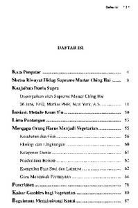
Figure 2.14 shows the Bit Error Ratio (BER) curves for the STBC scheme with 1 and 2 receive antenna configurations. The SNR at each receive antenna is defined as the ratio between the transmit power and the noise power, which is assumed to be equal for all antennas, i.e. SNRi = 10log10

P , for i = 1, 2. σv2

(2.34)

STBC achieves the same diversity level as MRC with a 3dB loss in BER. For example, the diversity order for STBC with 1 receive antenna can be calculated from Figure 2.14 using (2.23) as dSTBC,1 = 10 ×

5−3 = 2, 24 − 14

(2.35)

which is equal to the maximum diversity gain, dmax = M × N = 2. The 3dB loss is attributed to the power normalisation at the transmitter, i.e. for STBC each antenna radiates half the power transmitted by the one antenna in the case of MRC. As shown in [6], the algorithm can be trivially generalised to an arbitrary number of receive antennas, N , for higher diversity orders.

2.5.2

MMSE Decoding

The STBC decoding scheme proposed in [6] is only based on the channel gain and ignores the channel noise contribution to the received signal. This section derives an MMSE decoding approach for Alamouti’s STBC Scheme. Consider the two consecutive symbols picked up by one receive antenna as in (2.29):

¯ +v ˜r = Ha ˜ ,

(2.36)

} { where Raa = E aaH is the covariance matrix of the STBC coder input and Rvv = { } E vvH is the noise covariance matrix. For MMSE-STBC decoding, we assume the


28

0

10

No Diversity STBC 2x1 MRC 1x2 STBC 2x2 MRC 1x4

−1

10

−2

BER

10

−3

10

−4

10

5

10

15 SNR, [dB]

20

25

30

Figure 2.14: The BER curves for STBC and MRC. use of a matrix G:





( )  r1  ¯ +v ˆ a = G ˜ .  = G Ha r2∗

(2.37)

The resulting error vector is defined as

e=ˆ a − ρa,

(2.38)

leading to the MMSE

{ { }} tr E eeH } ) { ( ¯ H GH + |ρ|2 Raa . ¯ aa − ρRaa H ¯ H + Rvv GH − ρ∗ GHR ¯ aa H = tr G HR

ξ =

(2.39)

The quadratic expression of ξ can be minimised by differentiation with respect to (w.r.t) G [40],


29

( ) ∂ ¯ aa H ¯ H + Rvv GH − ρ∗ HR ¯ aa ξ = HR ∂G

(2.40)

and subsequently defining the optimum MMSE solution of the location where the gradient is zero, i.e. ( ) ¯ H HR ¯ aa H ¯ H + Rvv −1 . Gopt,MMSE = ρRaa H

(2.41)

Note that if Raa = σa2 I2 and in the absence of noise 

 ¯H = Gopt,MMSE|Rvv =0,Raa =σ2 I2 = ρ∗ H a

h∗1

−h2  ρ∗   , |h1 |2 + |h2 |2 h∗ h 1 2

(2.42)

which is the zero forcing solution and precisely what is used in standard STBC decoding as shown in 2.32. The scalar factor (|h1 |2 + |h2 |2 ) is absorbed into ρ∗ . To evaluate the performance of MMSE decoding, we define the SNR as the ratio between the afforded transmit power and noise power at the receiver

SNR =

tr {Raa } . tr {Rvv }

(2.43)

Computer simulations have been performed whereby the channel coefficients are drawn from a Rayleigh distribution with E {|h1 |2 } = E {|h2 |2 } = 21 . The simulation results averaged over 1000 channel realisations are shown in Figure 2.15. The MMSE ( ) ¯ aa H ¯ H + Rvv −1 , solution requires calculating the inverse of the M × M matrix HR which increases the complexity of the receiver and may not be practical if the matrix is ill conditioned. The results in Figure 2.15 suggest that the performance improvement is not sufficiently large over typical SNR values over the range of 5dB upwards to justify the effort. If the noise is imbalanced, i.e. E {|v1 |2 } ̸= E {|v2 |2 }, the performance does not change with respect to Figure 2.15. Similarly, using correlated noise whereby the noise


30

covariance matrix is not diagonal, does not result in any deviation from the results in Figure 2.15.

2.5.3

Generalised STBC

Alamouti’s STBC scheme was originally proposed for two branch transmit diversity, i.e. two transmit antennas. However, it can be generalised to an arbitrary number of antennas, [31, 28]. During one time slot, the encoder is supplied with k symbols. The symbols are transmitted from M antennas in p time periods. The rate of the code is defined as:

Rc =

k . p

(2.44)

The symbol streams transmitted from the different antennas are linear combinations of the mapped symbols a1 a2 , · · · , ak and their complex conjugates a∗1 , a∗2 , · · · , a∗k . The matrix of transmitted symbols is designed to fulfill the orthogonality condition similar to 2.26, ( ) SSH = η |a1 |2 + · · · + |ak |2 IM

(2.45)

where η is a constant. It is desirable to construct codes with a full rate, i.e. Rc = 1, due to their bandwidth efficiency. The design of STBC codes differs for real and complex symbol constellations, which will be discussed separately below.

2.5.3.1

Real Constellations

The following is an STBC code for real transmit constellations,


31

10 MMSE ZF

5

MSE / [dB]

0 −5 −10 −15 −20 −25 −5

0

5

10 SNR / [dB]

15

20

25

Figure 2.15: Mean squared error curves for MMSE and ZF solutions to space-time block decoding. 

 a1

a2

a3

a4

     −a2 a1 −a4 a3    S4 =     −a a a −a  3 4 1 2    −a4 −a3 a2 a1

for M = 4,

(2.46)

as in [31]. In general, the minimum number of time periods p to achieve full diversity is given by ( ) pmin = min 24η+ς

(2.47)

where 0 ≤ η, 0 ≤ ς ≤ 4, and 8η + 2ς ≥ M . Note that for any number of transmit antennas M = 2i where i ∈ N, an STBC code with rate Rc = 1 can be constructed to achieve full diversity at the receiver.

2.5.3.2

Complex Constellations

The following is an STBC code for complex symbol constellations [28]:


32



 a∗2

a∗3

0   a1   ∗ ∗  S13 =   −a2 a1 0 −a3    ∗ ∗ −a3 0 a1 a2

for M = 3, η = 1.

(2.48)

This code achieves full diversity with a rate of Rc = 43 . Note that the Alamouti code is the only code with rate Rc = 1 that archives full diversity. For any number of transmit antennas M > 2, an STBC code with rate Rc =

1 2

can be designed to achieve full

diversity for any complex constellation. Figure 2.16 shows the BER for different values of N . Compared to the BER curves in Figure 2.14, a higher diversity level is observed for the same number of receive antennas. Consider the case with 3 transmit and 1 receive antenna. The diversity level can be calculated from the BER curve according to (2.23) yielding the maximum diversity,

d3×1 = 10 ·

2.6

4−2 ≈ 3 = M N. 14 − 8

(2.49)

STBC for Multiple Users

One of the most important aspects of telecommunications is the ability to accommodate multiple users within the same medium. A number of different multiplexing schemes have been derived for this purpose including Time-Division Multiple Access (TDMA), Frequency Division Multiple Access (FDMA) and Space Division Multiple Access (SDMA), [41]. However, due to its capacity improvement and ability to accommodate all users within the same frequency band and at the same time, the most promising multiple access scheme is Code-Division Multiple Access (CDMA), [42, 43]. CDMA has been chosen as the main standard for 3G communication networks and is the first candidate for 4G networks, [44]. MIMO systems have demonstrated an enormous increase in system performance


33

BER curve for a 3 branch STBC system with a rate of 3/4.

0

10

STBC − 3x1 STBC − 3x2 STBC − 3x3 STBC − 3x4 No Diversity

−1

10

−2

BER

10

−3

10

−4

10

−5

10

−6

10

0

2

4

6 8 SNR, [dB]

10

12

14

Figure 2.16: STBC with 2 and 3 transmit and N receive antennas. over a conventional SISO setup. A lot of work has concentrated on combining MIMO and CDMA. Inspired by Alamouti’s Space-Time Block Coding, a transmit diversity scheme for CDMA systems was derived in [45], named Space-Time Spreading (STS). The STS scheme is briefly explained in this section, followed by a differential STS scheme introduced in [46, 47].

2.6.1

Space-Time Spreading

Inspired by the STBC coding scheme, Space-Time Spreading (STS) was introduced in [45] as a transmit diversity scheme for Wideband-CDMA systems. Consider a system with two transmit and M receive antennas. Similar to STBC, the source data is split into odd and even symbol sequences, s1 [n] and s2 [n], respectively. The signals transmitted from the two antennas are defined in the blocks s1 [n] =

√1 2

s2 [n] =

√1 2

[s1 [n] c1 + s∗2 [n] c2 ] [s2 [n] c1 −

s∗1

[n] c2 ] ,

(2.50)


34

where c1 and c2 are unit-norm orthogonal 2K × 1 codes, with K being the CDMA spreading gain. If only one code, c, is assigned to every user, the two codes can be [ ]T [ ]T defined as c1 = cT cT and c2 = cT − cT . Note that c1 and c2 are still orthogonal, cH 1 c2 = 0. The channel from the j th transmit antenna to the ith receive antenna is denoted hij [l, 0], where l is the chip index, and is assumed to be flat fading. Channel hij [l, 0] is also assumed to be stationary over one symbol period, i.e. 2K chips. Hence, the time index n will be dropped in subsequent derivations because a received data block is only dependent on a single transmitted block. The signal picked up by the ith receive antenna during one symbol period can be written as

ri = hi1 s1 + hi2 s2 + vi ,

(2.51)

where vi is additive white Gaussian noise. The received signals are then pre-multiplied by the Hermitian of the orthogonal codes c1 and c2 to produce the despread signals dji , d1i = cH 1 ri =

√1 2

[h1i s1 + h2i s2 ] + cH 1 vi

(2.52)

d2i = cH 2 ri =

√1 2

[−h2i s∗1 + h1i s∗2 ] + cH 2 vi .

For simplicity, let us define the following:









h2i   h1i  d1i  ¯ di =  ,  , Hi =  ∗ ∗ −h2i h1i d2i     H  c1 vi   s1  ˜i =  s =  .  , and v v cH s2 2 i


35

Using these definitions, (2.52) can be rewritten as 1 ¯ ˜i. di = √ H is + v 2

(2.53)

¯ H , gives Pre-multiplying dj by the Hermitian of the equivalent channel matrix, H j ¯ H dj = H j

¯ HH ¯ js √1 H 2 j

¯ Hv +H j ˜j

= =



√1 2

 |h1,j | + |h2,j |  0

√1 2

¯ Hv (|h1,j |2 + |h2,j |2 ) s + H j ˜j .

2

2

0 |h1,j | + |h2,j | 2

2

 ¯ Hv s + H j ˜j

(2.54)

The next step is to combine the signals retrieved from the different receive antennas through (2.54), which is achieved by averaging across all N decoded symbols,

ˆs[n] =

{M ∑(

¯ H dj H j

)

} /N.

(2.55)

j=1

It can be clearly observed from (2.54) that the source symbol sequences s1 [n] and s2 [n] have been decoupled by the receiver, and that maximum diversity gain has been achieved. Similar to STBC, STS can be derived for an arbitrary number of transmit antennas, as in [45]. However, the two branch code used here is the only full-rate code that achieves full diversity. Higher codes reduce the bandwidth utilisation of the system. The STS scheme assumes that the channel is stationary over the duration of 2K chips and that the channel is estimated perfectly at the receiver. The performance of STS has been analysed in [48, 49] in the presence of estimation errors.

2.6.2

Differential Space-Time Spreading

To overcome the need for channel estimation in STS, a differential technique was derived in [47] based on differential STBC (DSTBC) in [46]. The idea is to transmit a pilot


36

symbol, which is a symbol known a priori to the receiver, and recursively define the transmitted data based on this symbol. At the receiver, the pilot symbol is used to obtain an estimate of the channel, and then recursively recover the data. In order to characterise DSTBC, consider a system with two transmit and one receive antenna. Similar to STBC, the source data is split into odd and even symbol sequences a1 [n] and a2 [n]. These sequences are then differentially encoded to form the signals a ˜1 [n] and a ˜2 [n], respectively. At time instant n = 0, the known symbols a ˜1 [0] and a ˜2 [0] are transmitted from the two transmit antennas. At the following time instants, the transmitted symbols are recursively defined by    ˜1 [n − 1]  ˜1 [n]   a  a  [n − 1]   /pn ,   = a1 [n]   + a2 [n]     a ˜2 [n − 1] −˜ a∗1 [n − 1]  a ˜2 [n] 

where pn =



√

  







a ˜∗2

(2.56)

(|˜ a1 [n − 1] |2 + |˜ a2 [n − 1] |2 ) is used to normalise the power of the trans-

mitted symbols. After differential encoding, STS is performed to obtain the transmit signals, s1 [n] and s2 [n]. Similar to (2.50), the transmit signals are defined by s1 [n] =

√1 (˜ a 2 1

[n] c1 + a ˜∗2 [n] c2 )

s2 [n] =

√1 (˜ a 2 2

[n] c1 − a ˜∗1 [n] c2 ).

(2.57)

Using the same notation and making the same assumptions as in Section 2.6.1, the signal picked up by the ith receive antenna are given by

ri [n] = hi1 [n] s1 [n] + hi2 [n] s2 [n] + vi [n] ,

(2.58)

where vi [n] is additive white Gaussian noise. To retrieve the two transmitted signals, first despreading is performed using the Hermitian of the orthogonal codes assigned to


37

a specific user, d1i [n] = cH 1 ri [n] =

√1 2

[hi1 [n] s1 [n] + hi2 [n] s2 [n]] + cH 1 vi [n]

(2.59)

d2i [n] = cH 2 ri [n] =

√1 2

[−hi2 [n] s∗1 [n] + hi1 [n] s∗2 [n]] + cH 2 vi [n] .

This is followed by differential decoding. Let us define   R1i [n − 1] = 

[n − 1]  , d2i [n − 1]





 d∗1i

 R2i [n − 1] = 

d∗2i

[n − 1]  , d1i [n − 1]



  Ri [n] = 

d∗1i

[n]  . d2i [n] (2.60)

The differential decoding process is carried out by using two consecutive data blocks as follows: ˜s1i [n] = RH i [n] R1i [n − 1] ˜ 1i [n] , = αi,n s1 [n] + v

(2.61)

˜s2i [n] = RH i [n] R2i [n − 1] ˜ 2i [n] , = αi,n s2 [n] + v where αi,n = (|hi1 [n] |2 + |hi2 [n] |2 ) ·

√

|v1 [n − 1] |2 + |v2 [n − 1] |2 . The signals are then

averaged in the same way as in STS, [ ˆs [n] =

M ∑

] ˜si [n] /M,

(2.62)

i=1

where ˜si [n] = [˜s1i [n] ˜s2i [n]]T , although it may be possible to further enhance the system performance by combining the contributions in (2.62) weighted by the their SNRs as in MRC. Since the αi,n is a positive real number, it is safe to say that the transmitted signals have been recovered. Simulation results will be presented in 2.6.3 to compare the BER


38

performance of DSTS to that of STS.

2.6.3

Performance of STS and DSTS

Computer simulations were carried out to analyse the performance of STS and DSTS. The channel matrix is drawn from a slow fading correlated Rayleigh distribution as shown in Figure 2.1. Figure 2.17 shows the BER curves for the two schemes using different antenna configurations. It can be clearly observed that using more antennas at the receiver increases the error performance of both schemes dramatically. The BER of the DSTS scheme is 3dB worse than that of the STS scheme. The reason is the noise amplification inherent in the differential decoding process. The source of this 3dB penalty is analysed in detail in [46]. Even though the BER performance of DSTS is 3dB worse than that of STS, it is still an attractive scheme, since the STS simulation assumes perfect channel estimation, which is not the case in practice. The presence of channel estimation errors results in the two BER curves being brought closer together. Another advantage of the DSTS scheme is the ability to receive the transmitted data without the need for a channel estimator which reduces the complexity and ensures robustness of the system. However differential encoding requires a slow fading channel.

2.7

Concluding Remarks

This chapter has introduced the concept of space-time block coding, which utilises the extra capacity provided by MIMO to exploit diversity. Unlike multiplexing techniques, the aim of diversity schemes such as STBC is not in increasing the data rate but in improving the resilience of the transmission link to fading. Full diversity can be achieved by placing multiple antennas at the receiver and using MRC [5, 39]. However, this is not practical for the downlink scenario due to the limitation on the cost and size of the mobile terminals. STBC achieves the maximum diversity order by placing multiple


39

0

10

STS 2x1 STS 2x2 DSTS 2x1 DSTS 2x2

−1

BER

10

−2

10

−3

10

−4

10

2

4

6

8 10 SNR, [dB]

12

14

16

Figure 2.17: The BER curves for STS and Differential STS using BPSK modulation. antennas at the transmitter. Section 2.6 presented a general overview of space-time spreading, which effectively combines STBC and DS-CDMA, and the differential STS scheme, which does not requires channel state information. So far in the thesis, the channel matrix has been assumed flat fading. This is not true for most communications systems as the channel is usually frequency selective. The next chapter will present broadband solutions for Space-Time Block Coding.

Chapter 3 STBC for Broadband Channels In the previous chapter, we looked at Space-Time Block Coding (STBC), which maximises the diversity gain over flat fading channels. The performance of STBC drops if the channel is frequency selective, i.e. the delay spread is not negligible. The resulting Inter-Symbol Interference (ISI) has to be combatted in order to achieve the maximum diversity. This chapter reviews schemes which have been proposed in the literature to maximise the diversity gain over broadband channels.

3.1

Overview of Existing Schemes

Frequency selectivity of the channel destroys the orthogonality of the transmitted STBC ¯ H , as a matched streams. Hence, using the Hermitian of the effective channel matrix, H filter at the receiver is not sufficient to decouple the original sequences. Only two schemes have been proposed in the literature for combatting the effect of ISI on the MIMO diversity gain. Firstly, STBC can be combined with Orthogonal Frequency Division Multiplexing (OFDM) in order to create narrowband subcarriers which offer the same properties as the channels assumed for STBC in Chapter 2. Secondly, a block based scheme known as Time-Reversal STBC (TRSTBC). MIMO-OFDM has been widely used to divide the broadband channel into a number

40

CHAPTER 3. STBC FOR BROADBAND CHANNELS

41

of narrowband subchannels, where STBC is applied separately to mitigate the effect of fading, see [50, 51]. However, similar to the SISO case, MIMO-OFDM suffers from a very poor Peak-to-Average Power Ratio (PAPR) and sensitivity to frequency offsets, which leads to significant Inter-Carrier Interference (ICI). The remainder of this chapter analyses TRSTBC as introduced in [19, 21] and investigates blind equalisation methods for this broadband STBC approach.

3.2

Time-Reversal STBC

Recall from Section 2.5.1 that the channel was assumed to be flat fading, i.e. the frequency response of the channel is constant over the signal bandwidth. This assumption is invalid for communication systems where the coherence bandwidth of the channel is less than the bandwidth of the signal. The TRSTBC transmit diversity scheme, introduced in [19, 21], will be explained in this section. Simulation results will be shown at the end of this section to evaluate the TRSTBC scheme. Consider the transmission of a block of data whose length is 2La using a two transmit and one receive antenna configuration. The source data is divided into odd and even symbol sequences, denoted a1 [k] and a2 [k], respectively. In order to mitigate the effect of ISI, data is transmitted in blocks and guard periods are inserted between consecutive blocks. We define the sequences s1 [n] and s2 [n], whose structure is shown in Figure 3.1. The sequence P [n] is used as preamble and postamble. The length of P [n] is an integer Lp , which satisfies Lp > Lh , with Lh being the length of the longest multipath channel. The first part of transmission is called the regular burst, s[n], and the second part is called the reverse burst, due to the time reversion performed on the sequences −s∗2 [n] and s∗1 [n]. Notice that if the length of the source data block La = 1 and the length of the redundancy Lp = 0, the burst length Ls = 1 and this scheme reduces to Alamouti’s STBC. For the remainder of this section, assume La > Lp > 1. The data model of the TRSTBC system with two transmit and one receive antenna,


42

s[n] (a)

s1 [n] P [0]....P [Lp − 1]

a1 [0].....a2 [La − 1]

P [0]....P [Lp − 1]

s2 [n] P [0]....P [Lp − 1]

a2 [0].....a2 [La − 1]

P [0]....P [Lp − 1]

(b)

s1 [0] · · · s1 [Ls − 1]

−s∗2 [Ls − 1] · · · − s∗2 [0]

s2 [0] · · · s2 [Ls − 1]

s∗1 [Ls − 1] · · · s∗1 [0]

regular burst

reverse burst

Figure 3.1: Block structure in Time-Reversal STBC: (a) structure of the regular burst, (b) regular and reverse bursts. M = 2 and N = 1, is shown in Figure 3.2. The TR (·) and (·)∗ are non-linear functions denoting time reversal and complex conjugation, respectively. Considering the transmission of a specific block of data and assuming the channel is stationary over the regular and reverse bursts, we define the polynomial channel matrix 



h1 (z) h2 (z)  ¯ (z) =  H  , ∗ −1 ∗ −1 h2 (z ) −h1 (z )

(3.1)

where hi (z) is the z-transform of the frequency selective channel from the ith transmit antenna to the single receive antenna,

hi (z) •−−◦ hi [n] ,

i.e. hi (z) =

∞ ∑

hi [n] z −n .

(3.2)

(3.3)

n=−∞

¯ (z) are complex conjugated Note that the polynomials on the second row of matrix H and time reversed. As shown in Figure 3.2, the signal received during the regular burst is denoted r1 [n] and the signal received during the reverse burst is time-reversed and complex


h1 [n]

s1 [n]

43

v[n] r1 [n]

(·)∗

TR(·)

h2 [n]

s2 [n]

TR(·)

(·)∗

TR(·)

(·)∗

r2 [n]

-1

Figure 3.2: A 2 × 1 Time-Reversal STBC (TR-STBC) system. conjugated to produce r2 [n]. The vector of received signals is given by 



 r1 [n]  r[n] =   r2 [n] L∑ h −1 ¯ ν s[n − ν] + v[n], = H

(3.4)

ν=0

¯ ν is the ν th matrix valued coefficient of the polynomial channel matrix H ¯ (z), where H v[n] represents additive white Gaussian noise, and s [n] = [s1 [n] s2 [n]]T . It can be observed that the received signals contain contributions from the two transmitted signals. In other words, the detection of s1 [n] and s2 [n] is coupled. ˜ as the extension of the HermiDefine the para-Hermitian operator, denoted by (·), tian operator to polynomial matrices. Applied to a polynomial matrix, it transforms its rows into columns, conjugates all the entries and reverses the polynomials. The para-Hermitian of the channel matrix can be given by:  ( ) ˜ ¯ (z) = H ¯ H z −1 =  H 

 h∗1

−1

(z ) h2 (z)

h∗2 (z −1 ) −h1 (z)

 .

(3.5)

˜¯ (z) produces a diagonal matrix whose diagonal Pre-multiplying the channel matrix by H elements are identical:

CHAPTER 3. STBC FOR BROADBAND CHANNELS  ˜¯ (z) H ¯ (z) =  H    =  |

 h∗1

44 

−1

(z ) h2 (z)

h2 (z)   h1 (z)    h∗2 (z −1 ) −h1 (z) h∗2 (z −1 ) −h∗1 (z −1 )  d (z) 0  , 0 d (z) {z } D (z)

(3.6)

where ( ) ( ) d (z) = h∗1 z −1 h1 (z) + h∗2 z −1 h2 (z) .

(3.7)

¯˜ (z) can be used as a matched filter bank to decouple the transmitted Therefore, H data allowing equalisation to be carried out separately on the outputs y1 [n] and y2 [n], as shown in Figure 3.3. Ignoring the noise component, the output of the matched filter is given by





 y1 [n]  y[n] =   = y2 [n] =

L∑ h −1

˜¯ ν r[n − ν] H

ν=0 L∑ d −1

(3.8) Dj s[n − j]

j=0

where Ld is the length of the polynomial d (z) and Dj is the j th time slice of D (z). Thus, we can write

yi [n] =

L∑ d −1

d[l]si [n − l] for i = 1, 2,

(3.9)

l=0

where d[l] is the lth coefficient of d (z), which characterises the overall response of the channel and matched filter. This scheme can be trivially extended to an arbitrary number of receive antennas, N , for higher diversity gains. The channel matrix is generally defined similar to (3.1),


45

Channel Estimation

r1 [n]

-

r2 [n]

-

?

?

-

˜ (z) H

-

MLSE

?

- aˆ[n]

MLSE

Figure 3.3: Matched filtering and equalisation in TRSTBC. 



h1 (z) h2 (z)  ¯ (z) =  H  , h∗2 (z −1 ) −h∗1 (z −1 )

(3.10)

with

hi (z) = [hi1 (z) · · · hiM (z)]T

for i = 1, 2,

(3.11)

where hij (z) is the channel from the the j th transmit antenna to the ith receive antenna, and the received signals are represented by the vector

r[n] = [r11 [n] r21 [n] · · · r1N [n] r2N [n]]T .

3.2.1

(3.12)

Maximum Likelihood Sequence Estimation

The equalisation scheme chosen here is the Maximum Likelihood Sequence Estimation (MLSE), which is a form of Viterbi decoder, see [52]. More information on the maximum likelihood rule can be found in [21, 19].

Computer simulations were performed to evaluate the performance of Time-Reversal STBC with MLSE. QPSK modulated data was transmitted from two antennas over frequency selective channels. In the first experiment, one and two receive antennas were used to pick up the transmitted data and perform combining, decoding, and equalization. The channel is assumed to be stationary. The BER is averaged over an


46

0

10

MLSE 2×1 MLSE 2×2 −1

10

−2

BER

10

−3

10

−4

10

−5

10

0

2

4

6 8 SNR, [dB]

10

12

14

Figure 3.4: The BER curves for TR-STBC using different antenna configurations. ensemble of 100 Rayleigh channel realisations, the power delay profile for the channel is given in Table 2.1. Figure 3.4 shows the BER curves for the two antenna configurations. The second experiment looks at the effect of non-stationarity of the channel on a 2 × 2 TRSTBC system. The length of the data bursts is set to Lv = 236 and the length of the preamble and postamble is set to Lp = 10, making the overall length of the regular and reverse bursts 512 symbols. The channel realisations are drawn from a correlated Rayleigh distribution with normalised Doppler shift fd = 100, which corresponds to a vehicular speed of 55km/h assuming a carrier frequency of 2GHz and a transmission bandwidth of 50KHz. The channel is assumed to be stationary for a duration Qs symbol periods. The same power delay profile is used as in the first experiment. Figure 3.5 shows the BER curves for different value of Qs assuming the channel variation can be tracked at the receiver. It can be observed that the effect of channel non-stationarity on the performance of the MLSE is not considerable. However, the accuracy of timevarying channel identification is inversely proportional to the rate of variation Qs . Thus for a fast time-varying channel, a noisy channel estimate is obtained, which degrades the performance as will be shown in the next section.


47

−1

10

MLSE − L =236, Q =128 v

s

MLSE − L =236, Q =256 v

−2

s

MLSE − Lv=236, Qs=512

10

−3

BER

10

−4

10

−5

10

−6

10

0

1

2

3

4 SNR, [dB]

5

6

7

8

Figure 3.5: BER curves for TRSTBC for different values of the stationarity variable Qs .

3.2.2

Effect of Noisy Channel Estimation

So far in this thesis, the availability of perfect channel state information (CSI) has been assumed at the receiver. This generally implies the inclusion of redundancy, commonly known as training, in the transmitted data. Based on the measured response of the channel to the training sequence, the channel can be estimated at the receiver using a number of algorithms. A finite measurement interval and the presence of channel noise lead to a noisy channel estimate as opposed to a perfect one. This estimation error generally reduces the performance of the system. The channel imperfection is modeled by a white Gaussian error, E (z), with variance ¯ (z) to produce the inaccurate estimate σe2 added to H

ˇ (z) = H ¯ (z) + E (z) . H Pre-multiplying the channel by the para-Hermitian of the estimate yields

(3.13)


˜ ˜ H ¯ (z) = H(z) ¯ ¯ (z) + E(z) ˜ H ¯ (z) ˇ (z) H H   0   d (z) ˇ =   + E(z). 0 d (z)

48

(3.14)

ˇ (z −1 ) where d (z) is defined in (3.7). Even in the absence of noise, the additive matrix E makes the product a non diagonal polynomial matrix, i.e. the entries will not be fully decoupled. Simulations were performed to evaluate the robustness of TRSTBC with MLSE to channel estimation errors. A 2 × 2 MIMO system is assumed with QPSK symbol mapping at the transmitter. Figure 3.6 shows the BER curves corresponding to different values of the variance σe2 . A considerable degradation is observed, even for a variance as small as 0.1, i.e. 10dB. Note that the BER curve tends to level out at high SNRs. This is due to the noise variance being negligeable compared to the variance of the estimation error, σv2 ≪ σe2 . Figure 3.7 shows the BER with respect to the estimation error variance σe2 for 6dB SNR. The BER ranges from 10−4 in the absence of estimation errors to 10−1 when the variance reaches 0.5, i.e. 3dB. In order to overcome the degradation associated with imperfect channel estimation, a blind receiver was derived in [20] based on the Constant Modulus (CM) criterion, in [53]. This algorithm will be investigated in Section 3.3.

3.3

CM Equalisation for TR-STBC

In most STBC systems the availability of CSI is assumed at the receiver, which generally implies channel estimation based on training. The channel estimate is used to equalise the received signal by reversing the effect of the channel. The periodical transmission of a training sequence reduces the throughput of the system and is not practical in fast time-varying channels. Therefore blind and semi-blind equalisation algorithms are investigated in this thesis. The most commonly used blind equaliser is the constant


49

−1

10

−2

10

−3

BER

10

−4

10

MLSE − Perfect CSI MLSE − σ2=0.05

−5

10

MLSE − σ2=0.1 MLSE − σ2=0.2

−6

10

0

2

4

6 SNR, [dB]

8

10

12

Figure 3.6: BER curves for TRSTBC with channel estimation errors.

−1

10

−2

BER, [dB]

10

−3

10

−4

10

0

0.05

0.1

0.15

0.2 0.25 0.3 0.35 σe of Estimation Error

0.4

0.45

0.5

Figure 3.7: BER curve with respect to the variance of the channel estimation error for 6dB SNR.


50

modulus algorithm (CMA) [53, 54, 55]. It is based on the constant modulus property of the transmitted signal, although it still converges for non-constant-modulus source constellations [56]. CMA has been proven to be robust and is similar to the Least Mean Square (LMS) algorithm in its complexity. In the following, we first review the derivation and analysis of the CMA. Thereafter, we state the signal model for TRSTBC, which has motivated the modification of the CMA, known as tap-constrained CMA as proposed in [20]. This algorithm exploits the structure of the TRSTBC transmission by placing a constraint on the multiple equaliser vectors, hence the term tap-constrained.

3.3.1

The Constant Modulus Algorithm

Blind equalisation algorithms employ a priori knowledge about the transmitted signal to remove the effect of Inter-Symbol Interference (ISI). The objective of the CM algorithm is to restore the output signal to a form, which on average, has a constant modulus equal to that of the source constellation. This can be done by adapting the weight vector of the adaptive filter w [n] to minimise the following cost function,

ξ = E{(|y [n] |q1 − γ q1 )q2 }.

(3.15)

Over the remainder of this thesis, q1 and q2 are assumed to be equal to 2 yielding the cost function ξ = E{(|y [n] |2 − γ 2 )2 },

(3.16)

where γ is the constant modulus, y [n] is the output symbol

y [n] = wH [n] rn ,

(3.17)


51

and rn represents the transversal delay line of the filter rn = [r [n] r [n − 1] · · · r [n − L + 1]]T .

(3.18)

Given a cost function and a filter structure, there are a number of methods that could be followed to obtain an update equation for the equaliser. The gradient descent method, known for its simplicity and robustness, has been chosen to update the weight vector w, w [n + 1] = w [n] − µ∇w∗ ξn ,

(3.19)

where µ is a positive step size and ▽w∗ denotes the gradient operator with respect to w∗ . Note that the CMA cost function in (3.16) is biquadratic, thus has local minima. Gradient methods such as (3.19) are generally not well suited for this purpose, but are widely used in the literature nonetheless. Using Wirtinger’s complex valued calculus explained in Appendix A, it can be verified that [ ] ▽w∗ ξn = E{[|y [n] |2 − γ 2 ] . ▽w wH [n] rn rH n w [n] } = E{[|y [n] |2 − γ 2 ] rn rH n w [n]}

(3.20)

= E {[|y [n] |2 − γ 2 ] y ∗ [n] rn } . We following a stochastic gradient approach similar to the Least Mean Square (LMS) algorithm using an estimate of the cost function ξˆn . In the simplest case, the instantaneous estimate of the cost function is obtained by removing the expectation operator, yielding ∇w∗ ξˆn = [|y [n] |2 − γ 2 ] y ∗ [n] rn ∗

(3.21)

= e [n] rn , where e [n] = y [n] [|y [n] |2 − γ 2 ]. Equation (3.19) then becomes w [n + 1] = w [n] − µe∗ [n] rn .

(3.22)


52

Figure 3.8: The cost function ξˆ as a function of a complex valued single wight w0 . Figure 3.8 shows the cost function of the CM algorithm as a function of a single weight w0 with QPSK modulation and in the absence of noise. It can be seen that the cost function experiences a manifold of optimum solutions that lie on the circle that is centered at the origin with a radius equal to the constant modulus γ. The reason for this is the insensitivity of the CM algorithm to phase variations as it only corrects the amplitude of the received signal. A key factor in the performance of the constant modulus algorithm is the initialization of the weight vector w [n]. The method that has been proven most effective is the single spike initialization, in which all the taps are set to zero except the first or central tap. The value of the spike as well as its location may affect the convergence and steady-state mean square error (MSE) of the equaliser due to the presence of local minima in the cost function, see [54] for examples.

3.3.2

Data Model

Similar to [20], let us consider a system with two transmit and two receive antennas, although this can be easily generalized to N receive antennas. The transmitted data is divided into two sets of symbols a1 [n] and a2 [n], as explained in the previous chapter.


53

Data is transmitted in bursts. During the regular burst, s1 [n] and s2 [n] are transmitted from first and second antennas, respectively. During the reverse burst, the sequences are time reversed and conjugated in the way shown in Figure 3.1. The data model is shown in Figure 3.9. Let r [n] be the received signal of dimension 4 × 1, 

 r [n]   11    r˜21 [n]    r [n] =  ,  r [n]   12    r˜22 [n]

(3.23)

where ri1 [n] and ri2 [n] are the signals picked up by the ith antenna during the regular and reverse modes of transmission, respectively. Note that the signals received during the second phase of transmission are complex conjugated and time reversed to produce r˜12 [n] and r˜22 [n]. The vector r [n] can be written as

r [n] =

L∑ h −1

H[0, ν]s [n − ν] + v [n] ,

(3.24)

ν=0

where v [n] is the additive white Gaussian noise vector, s [n] = [s1 [n] s2 [n]]T , and Hν is the ν th time slice of the effective channel transfer function 







h2 (z)  h1 (z)   hi1 (z)  H (z) =   , with hi (z) =  , h∗2 (z −1 ) −h∗1 (z −1 ) hi2 (z)

(3.25)

where hij (z) is the channel from the j th transmit antenna to the ith receive antenna. The length of the channels is assumed to be identical, denoted Lh . As shown in Figure 3.10, two space-time equalisers, w1 [n] and w2 [n], are used to retrieve the transmitted data. Each space-time equaliser consists of four adaptive FIR filters of length Lw . At the nth iteration, the weight vector of the ith space-time equaliser


54

v1 [n]

h11 (z −1 )

r11 [n]

TR

h21 (z −1 )

*

r12 [n]

a1 [n] a2 [n]

TRSTBC h12 (z −1 )

r21 [n]

TR

h22 (z −1 )

*

r22 [n]

v2 [n]

Figure 3.9: Data Model for a 2x2 TR-STBC system. is given by



w∗i,11

[n]    w∗ [n]  i,21 wi [n] =   ∗  wi,12 [n]  w∗i,22 [n]

     ,   

(3.26)

and the corresponding output is

yi [n] = wH i [n] rn ,

(3.27)

where the regressor vector of the equaliser is given by, [ ]H H H H rn = r H , 11,n r21,n r12,n r22,n

(3.28)

with rji,n = [rji [n] rji [n − 1] · · · rji [n − L + 1]]T .

3.3.3

Tap-Constrained CMA

To blindly retrieve the transmitted signal at the receiver, the redundancy introduced by TRSTBC is exploited. A tap-constrained CM algorithm, which will be explained in this section, was derived in [20] for TRSTBC systems.


r11 [n]

w1,11 (z)

r12 [n]

w1,21 (z)

55

y1 [n] r21 [n]

w1,12 (z)

r22 [n]

w1,22 (z)

w2,11 (z)

w2,21 (z) y2 [n] w2,12 (z)

w2,22 (z)

Figure 3.10: CMA Equalization for TR-STBC. The para-Hermitian of the effective channel matrix is given by  ˜¯ −1 ) =  H(z 

 h∗11 (z −1 )

h∗12 (z −1 )

h21 (z)

h22 (z)

h∗21 (z −1 ) h∗22 (z −1 ) −h11 (z) −h12 (z)

 .

(3.29)

Similar to (3.6), pre-multiplying the effective channel matrix by its para-Hermitian yields





0   d (z) ˜¯ −1 )H(z) ¯ H(z = . 0 d (z) | {z } D (z)

(3.30)

From (3.30), it can be observed that D (z) is diagonal, which means the signals radiated from the two transmit antennas, i.e. s1 [n] and s2 [n], can be ideally decoupled when full channel information is available at the receiver. Another observation is that the diagonal elements of D (z) are identical, which means the equalisers needed for s1 [n] and s2 [n] after matched filtering are identical. Since the diagonal elements d (z) are symmetric in time, the total response of the matched filter and equaliser should be


56

˜¯ identical to H(z). From these observations, a tap constraint can be placed on the CMA weight vectors as follows, [ ∗T ]T T T q11 [Lh − 1 − n] q∗T 12 [Lh − 1 − n] q21 [n] q22 [n] [ ]T ∗T T T w2 [n] = q∗T , 21 [Lh − 1 − n] q22 [Lh − 1 − n] − q11 [n] − q12 [n]

w1 [n] =

(3.31)

˜¯ where q11 , q12 , q21 , and q22 are vector quantities obtained from H(z) in (3.29). For example,



 ∗ h [n, L − 1] h  11    ∗  h [n, Lh − 2]  11   q∗11 [Lh − 1 − n] =  . .   . .     h∗11 [n, 0]

(3.32)

This observation leads to the following relation between w1 [n] and w2 [n] w2 [n] = PT w∗1 [n] ,

where

     P=   

0

0

−˜ILw 0

0

0

0

−˜ILw

˜ILw 0

0

0

˜ILw 0

0

0

(3.33)

     ,   

(3.34)





 0 1  with ˜ILw being the reverse-identity matrix of size Lw × Lw , e.g. ˜I2 =  . 1 0 The cost function for the two space-time equalisers is given by, ξ = ξ1 + ξ2 2

2

(3.35)

= E{(|y1 [n] |2 − γ 2 ) } + E{(|y2 [n] |2 − γ 2 ) }, where γ is the constant modulus of the PSK constellation assumed at the transmitter.


57

According to the stochastic gradient method, w1 [n + 1] = w1 [n] − µ∇w1∗ ξˆ [ ] = w1 [n] − µ ∇w1∗ ξˆ1 + ∇w1∗ ξˆ2 .

(3.36)

where ξˆ is derived from ξ in (3.35) by dropping the expectation operator. Similar to the derivation of the CMA in Section 3.3.1, it can be verified that ∇w1∗ ξˆ1 = [|y1 [n] |2 − γ 2 ] y1∗ [n] rn = e∗1 [n] rn

(3.37)

and ∇w1∗ ξˆ2 = [|y2 [n] |2 − γ 2 ] y2 [n] Pr∗n =

e2 [n] Pr∗n

(3.38)

with the matrix P as defined in (3.34). Substituting (3.37) and (3.38) into (3.36) gives

w1 [n + 1] = w1 [n] − µ [e∗1 [n] rn + e2 [n] Pr∗n ] ,

(3.39)

whereby w2 [n + 1] is calculated from w1 [n + 1] according to (3.33). This defines the update operation of the weight vectors w1 [n] and w2 [n] at the nth iteration. A summary of the algorithm is listed in Table 3.1.

3.3.4

Tap-Constrained CMA Receiver Performance

Computer simulations have been used to compare the performance of the Tap-Constrained CMA equalizer with that of the ideal case presented in Section 3.2.1, where full CSI is available and MLSE is used. The length of s1 [n] and s2 [n] is set to 256 symbols and QPSK modulation is used to form the signal set {±1 ± j}. The BER was calculated over 1000 channels drawn from a correlated Rayleigh distribution corresponding to a vehicular speed of 55km/h. A 15-tap transversal filter (FIR) per equalizer wi,j is used. As mentioned in Section 3.3.1, choosing the optimum initialization of the weight vector


58

5 0 −5

MSE, [dB]

−10 −15 −20 −25 −30 −35 −40

0

500

1000

1500

2000

2500 3000 Iteration

3500

4000

4500

5000

Figure 3.11: TR-STBC Constant Modulus equalisation, MSE curve averaged over 1000 channel realisations.

0

10

TRSTBC−MLSE TRSTBC−CMA − N=256 −1

10

−2

BER

10

−3

10

−4

10

0

2

4

6 8 SNR, [dB]

10

12

14

Figure 3.12: TR-STBC Constant Modulus equalization, BER curve averaged over 1000 channel realisations.


59

Recursion: Update vector rn y1 [n] = wH 1 [n] rn y2 [n] = wT1 [n] P∗ rn ei [n] = [|yi [n] |2 − γ 2 ] yi [n] for i = 1, 2 w1 [n + 1] = w1 [n] − µ [n] [e∗1 [n] rn + e2 [n] Pr∗n ] Table 3.1: Summary of the Tap-Constrained CMA for TRSTBC. w1 [n], and consequently w2 [n], is crucial for the best performance of CMA. The central spike technique has been chosen for initialising w1 [n]. The step size µ = 3 × 10−4 was chosen as it gave the best stable convergence. Figure 3.12 shows the BER curve for the Tap-Constrained CM algorithm compared to the MLSE algorithm in Section 3.2.1. Figure 3.11 shows the Mean Square Error (MSE) over time. Due to the slow convergence of the CM algorithm, long bursts are required in order to achieve a desirable MSE level. Since the channel is assumed to be stationary over the duration of two bursts, the algorithm might not be suitable for nonstationary channels. In the following section, different variations of the TRSTBC-CMA will be explored in order to strive for faster convergence.

3.4

Fast Converging Implementations

This section presents three fast converging variations of the TRSTBC-CMA based on the conjugate gradient approach, Newton’s search method, and the Matched-PDF method. Simulation results will be presented at the end of the section to study the advantages and disadvantages of the different methods in terms of convergence speed, steady state BER, and computational complexity.


3.4.1

60

The Conjugate Gradient Search Method

This section describes the conjugate gradient (CG) search method and develops an adaptive implementation for the TRSTBC-CMA based on [57]. The notation used here is consistent with literature on conjugate gradient algorithms while retaining standard notation for e.g. the weight vector. In general, a linear system of equations is given by

Ax = b,

(3.40)

where A is an Lw × Lw matrix, x is a variable vector, and b is a vector of unknown variables. The optimum least squares solution, xopt , for the linear set of equations minimises the quadratic function

Q(x) = xT Ax − xT b.

(3.41)

The shape of the quadratic function depends on the matrix A. If A is positive definite, the parabola has a single minimum, whereas if A is negative definite, it will have a single maximum. The word semi-definite is used where the rank-deficient case is included, and the function may have a manifold of solutions. Assuming A is positive semidefinite, the function Q (x) can be minimised iteratively using a search method of the form

x [n + 1] = x [n] + µn g [n] ,

(3.42)

where µn is the step, and g [n] is the direction vector at time n, [58]. In words, the estimate of xopt is refined by taking a step in a certain direction. The simplest and most commonly used direction is the negative gradient of the quadratic function, commonly referred to as the gradient descent method. This method is simple and robust. However, if the condition number κ (A) =

λ1 (A) λn (A)

is large, the gradient is dominated by the

eigenvector selection to the largest eigenvalue, and converges slowly in the direction of


61

weaker modes. Taking multiple steps in the same direction can be prevented by drawing the directions from a set of A-conjugate vectors [58]. Two direction vectors g [i] and g [j] are said to be A-conjugate if gT [i] Ag [j] = 0, ∀i ̸= j.

(3.43)

In [57], the search direction is defined recursively by

g [l] = −p [l] + ℓl−1 g [l − 1] ,

(3.44)

where p [l] is the gradient vector and ℓl−1 is suitably chosen to ensure A-conjugacy of g [l] and g [l − 1] , g [l − 2] , . . . , g [0]. The same update equation can be used for the first space-time equaliser as in 3.36. The cost function is estimated over a window of Lw symbols, as in [57]. The gradient w.r.t. w1∗ is given by

∇w1∗ ξˆ =

Lw −1 { ∗ } 2 ∑ e1 [n − Lw ] rn−Lw + e2 [n − Lw ] Pr∗n−Lw . Lw i=0

(3.45)

For every new data input, m = min(L, Lw ) iterations are performed by the CG approach. The CG recursion is identical to [57, 59]. A description of the algorithm is given in Table 3.2.

3.4.2

Newton’s Search Method

The form of Newton’s algorithm is given in [60] as: w1 [n + 1] = w1 [n] − µR−1 rr ▽w1∗ ξ;

(3.46)

Under the following ideal conditions, using Newton’s algorithm leads to the optimum weight vector wopt in a single step:


62

Compute: Step 1:

p [0] = ▽ξˆ (w0 ) ,f [0] = w0 − p [0] ,u [0] = ▽ξˆ (f [0]) Set g [0] = −p [0]

For l = 0, 1, · · · , m − 1 (a) wl+1 = wl +

pH [l]g[l] g [l] (wl −u[l])

gH [l]

(b) Compute: ( ) p [l + 1] = ▽ξˆ wl+1

Step 2:

f [l + 1] = wl+1 − p [l + 1] u [l + 1] = ▽ξˆ (f [l + 1]) (c) If l < (m − 1), g [l + 1] = −p [l + 1] +

Step 3:

pH [l+1]p[l+1] g [l] pH [l]p[l]

Replace w0 by wm and go back to step 1.

Table 3.2: The adaptive Conjugate Gradient algorithm. 1. µ = 12 . 2. Exact knowledge of the gradient vector, ▽wi∗ ξ, at each iteration. 3. Exact knowledge of the received signal’s inverse correlation matrix R−1 rr . Using a step size less than

1 2

increases the number of steps required, but the algorithm

still proceeds in a straight path towards the optimum wopt . Since exact knowledge of the cost function, ξ, cannot be obtained in practice, a noisy estimate is used instead. Furthermore, the third condition cannot be realised in real time communication systems so an estimate of R−1 is used, hence the name Quasi-Newton. The weight vector update


63

equation becomes ˆ ˆ −1 [n] ∇w∗ ξ. w1 [n + 1] = w1 [n] − µR 1 3.4.2.1

(3.47)

The Fast Quasi Newton Implementation

In this section, the same data model from section 3.3.2 is used. From equations 3.37 and 3.38, the gradient for the estimated tap-constrained CM cost function is given by ∇w1 ξˆn = e∗1 [n] r [n] + e2 [n] Pr∗ [n] ,

(3.48)

[ ] ei [n] = |yi [n] |2 − γ 2 yi [n] for i = 1, 2.

(3.49)

where

The covariance matrix Rrr of a vector rn is defined as the expectation of the inner product of rn with its Hermitian, Rrr = E{rn rH n }.

(3.50)

ˆ rr [n], of the covariance matrix is used. Since Rrr is not known a priori, an estimate, R ˆ rr [n + 1] is defined recursively by Similar to [61, 62, 63], R ˆ rr [n + 1] = αf qn R ˆ rr [n] + (1 − αf qn )rn rH , R n

(3.51)

where αf qn is a number between 0 and 1, referred to as the remembrance factor. The ˆ rr [n] and its value of αf qn allows a trade-off between the the convergence speed of R ˆ rr [0] is set to the identity matrix, steady-state error. In the initialization stage, R ˆ rr [0] = I4Lw , and the input r [n] is set to zero for all n < 0. R ˆ rr [n] is a complex operation. A Calculating the inverse of the covariance matrix R Fast Quasi-Newton algorithm was derived in [63], which decreases the complexity from O(L2w ) to O(Lw log(Lw )) in the SISO case. The idea is that the input to an adaptive


64

Define matrix P (i)

w1 = 0, ∀i ̸= centre Initialization:

ˆ rr [0] = I4Lw R ( ) ˆ rr [0] Rinv = inverse R

Update vector rn y1 [n] = wH 1 [n] rn y2 [n] = wT1 [n] P∗ rn ei [n] = [|yi [n] |2 − γ 2 ] yi [n] for i = 1, 2 Recursion: µ [n] =

1 4[rH Rinv r+δ]

ˆ rr [n + 1] = αf qn R ˆ rr [n] + (1 − αf qn )rn rH R n ˆ −1 [n] , for n an integer multiple of Lw Rinv = R rr w1 [n + 1] = w1 [n] − µ [n] Rinv [e∗1 [n] rn + e2 [n] Pr∗n ] Table 3.3: Summary of the Fast Quasi-Newton TRSTBC-CMA algorithm. system is in theory required to be stationary, although it might change slightly in practice. It can be verified that an auto-correlation estimate which is accurate at time n will remain accurate until time n + Lw − 1, which means the inverse Rinv [n] need only ˆ be calculated every Lth w iteration. The Toeplitz structure of matrix Rrr [n] can also be exploited to reduce the complexity of the inversion using low complexity methods such as the Livinson-Durbin Recursion (LDR), [64], . Similar to [65], the inverse of the covariance matrix, Rinv , is also used to adaptively update the step size µ [n], µ [n] =

1 4 [rH n Rinv rn + ϵ]

,

(3.52)


65

where ϵ is a small number compared to the product rH n Rinv rn . A summary of the Fast Quasi Newton TRSTBC-CMA is shown in Table 3.3.

3.4.3

PDF-Fitting

This section considers a new blind equalisation scheme for TRSTBC, based on [66]. The PDF-fitting algorithm utilises knowledge of the transmitted constellation and its probability density function (PDF) at the receiver by forcing the equaliser output to exhibit the same characteristics. This has been proven to achieve faster convergence and better residual ISI for non-constant modulus constellations than the CMA, [66]. The idea is that the distribution of the data contains more information than the statistics employed by the CMA [67]. The received signal is assumed to be corrupted by additive white Gaussian noise. The cost function for the 2 × 2 TRSTBC equaliser can be given by

ξP DF =

2 {ˆ ∑ i=1

+∞

(

−∞

)2 } fYi2 (z) − fSi2 (z) dz ,

(3.53)

{ } { } where Yi2 = |yi [n]|2 , Si2 = |si [n]|2 , and the function fX (z) denotes the PDF of X at z. Similar to [67], we use the Parzen window estimator, proposed in [68], to estimate the PDFs:

) 1∑ ( Gσ z − |yi [n − i]|2 fYi2 (z) = L i=0 L−1

i = 1, 2,

(3.54)

where σ is the standard deviation of the Gaussian kernel function Gσ (z). For consistency, the PDF of the transmitted symbols is calculated using the same estimator

fYi2 (z) =

m ∑

( ) Pai Gσ z − |ai |2 ,

(3.55)

i=1

where Pai is the probability of symbol ai , which is drawn from a constellation of size m. Following the same steps as in [67], the gradient for the new cost function can be


66

Update vector rn y1 [n] = wH 1 [n] rn y2 [n] = wT1 [n] P∗ rn Recursion:

ei [n] = [|yi [n] |2 − γ 2 ] yi [n] for i = 1, 2 w1 [n + 1] = w1 [n] − µ ˜P DF [e∗1 [n] a1 [n] rn + e2 [n] a2 [n] Pr∗n ] , −

2

(|yi [n]|2 −γ 2 )

where, ai [n] = e

2σ 2

, for i = 1, 2

Table 3.4: Summary of the PDF-Fitting algorithm for TRSTBC. shown to be

∇w1 ξˆP DF

1 =√ 2π

{ e∗1 [n] rn e

(

− |y1 [n]|2 −γ 2 2σ 2

)

2

+ e2 [n] Pr∗n e

(

− |y2 [n]|2 −γ 2 2σ 2

2

)

} ,

(3.56)

where the summation in (3.55) has been dropped and only the modulus of yi [n] is corrected. Given a step size µP DF , the update equation for the matched PDF equaliser is given by w1 [n + 1] = w1 [n] − µ ˜P DF ∇w1 ξˆP DF ,

(3.57)

and w2 [n + 1] is derived from w1 [n + 1] similar to the TRSTBC-CMA. A summary ˜P DF = of this algorithm is given in Table 3.4, where the factor √12π is absorbed into µ √ 2πµP DF . Note that the gradient of the derived PDF-fitting algorithm is identical to the standard STBC-CMA multiplied by the exponential term. Hence, as will be seen in Section 3.4.5, their complexities are very similar.


67

5 0 Matched−PDF

−5

MSE, [dB]

−10 −15

Boray − CG

−20 TRSTBC−CMA

−25 −30 FQN

−35 −40

0

1000

2000

3000

4000

5000

Iteration

Figure 3.13: MSE curves for the different implementations of the TRSTBC-CMA.

3.4.4

Performance Comparison of the Different Equalisers

Computer simulations have been carried out to evaluate the performance of the pro√ posed equalisers. QPSK symbol mapping was used with a modulus equal to 2. An appropriate burst length was chosen to allow time for the equalisers to converge. 1000 channel realisations were drawn from a correlated Rayleigh distribution with a normalised maximum Doppler frequency fd = 100Hz. Subequalisers of order 15 were used in the simulations. The first space-time equaliser w1 [n] was initialised using the central spike technique and the step size was fixed at 3 × 10−4 . The equaliser specific parameters were intialised according to Table 3.5. Figure 3.13 shows the MSE curves for the different TRSTBC equalisers. It can be clearly observed that the proposed implementations outperform the standard tapconstrained CMA in terms of convergence speed. The FQN algorithm converges faster than all other methods, followed closely by the PDF-fitting approach. Figure 3.14 shows the BER achieved by the different equalisers with respect to the burst length at SNR = 10dB. The channel was varied after two bursts of size 256 symbols. The channel coefficients were drawn from a 3-tap doubly dispersive Rayleigh

CHAPTER 3. STBC FOR BROADBAND CHANNELS Conjugate Gradient Lw = 10

68

FQN-CMA

PDF-Fitting

αf qn = 0.999 ϵ = 0.002 ˆ rr [0] = I4Lw R

σ=1 µP DF = 2 × 10−3

Table 3.5: Simulation parameters for the different blind equalisers. 0

10

Constant Modulus Conjugate Grad Fast Quasi−Newton Matched−PDF CMA

−1

10

BER

−2

10

−3

10

−4

10

50

100 150 200 250 300 Length of Burst, Excluding Redundancy

350

400

Figure 3.14: BER for the different implementations of the TRSTBC-CMA, SNR = 10dB. channel with maximum Doppler frequency fd = 100Hz, corresponding to a vehicular speed of 55km/h. A gradual decrease in the BER is observed as we move from one equaliser to the other in the same sequence as in the MSE curves. This translates to faster adaptation to channel variations. However, even with the FQN implementation, a burst size of at least 150 symbols is required to achieve a BER lower than 10−2 . This implies the channel has to be stationary over a duration longer than 300 symbols. Hence, TRSTBC with blind equalisation is generally not suitable for fast time-varying channels.

CHAPTER 3. STBC FOR BROADBAND CHANNELS CM Algorithm Conjugate Gradient 4Lst + 6

47Lst + 116

FQN-CMA 4L2st + 6Lst + 23

69 Matched-PDF-Fitting

+LDR/L

4Lst + 8

Table 3.6: Complexity of the different equalisers, in terms of accumulative multiplications and the Levinson-Durbin recursion (LDR).

3.4.5

On the Complexity of the Algorithms

Section 3.4.4 showed how the derived algorithms achieved faster convergence and lowered the bound on the burst length. However, to fairly evaluate the performance gain, the complexity of the different algorithms must be considered. Table 3.6 shows the number of Multiply-Accumulate (MAC) operations required by the proposed algorithms in terms of the ST equaliser order Lst = M N Lw = 4Lw for every iteration n. The multiplication by matrix P has been ignored because it is a permutation matrix that can be implemented by indexing. In Table 3.6, the number of recursions for the CG scheme is assumed to be m = 5. The division operation can be performed in a number of MACs equal to the wordlength, which is assumed 16 here. In the FQN-CMA column, the Levinson-Durbin Recursion is evaluated to invert the covariance matrix once every Lw iterations. The PDF-Fitting algorithm requires evaluation of the exponentials in addition to the complexity in Table 3.6. The exponential term is assumed to be evaluated using a look-up table, where the accuracy of the result depends on the size of memory allocated to the table. Hence, the added complexity compared to the standard STBC-CMA is only one MAC operation for each output. Figure 3.15 shows the complexity plot in terms of the order Lw . When weighting the gain against complexity, the PDF-Fitting algorithm stands out. The complexity difference between the standard STBC-CMA and the PDF-Fitting algorithm is very negligible, yet its performance approaches that of the FQN-CMA.


70

5

10

CMA CG−CMA FQN−CMA Matched−PDF

4

Complexity, [MACs]

10

3

10

2

10

1

10

2

4

6

8

10 12 14 Filter Length (Lw)

16

18

20

Figure 3.15: Number of MACs required per iteration for proposed algorithms.

3.5

Concluding Remarks

This chapter has looked at space-time coding for frequency selective channels. Most of the schemes proposed in the literature are block based including OFDM-STBC and the technique discussed in this chapter, namely Time-Reversal STBC, [21, 19]. A blind CM receiver was proposed in [20] for TRSTBC. The tap-constrained CM receiver performs well over stationary channels but suffers from slow convergence. Different implementations of the blind receiver were investigated in this chapter. The equaliser with the fastest convergence is based on the Fast Quasi-Newton method. Even with the fastest converging equaliser, a burst of significant length was required to achieve desirable BER levels. This renders the TRSTBC scheme unsuitable for use over fast time-varying channels. Furthermore, long bursts require a larger memory at the receiver, which is not always feasible. Therefore, in the next chapter, a non-block based CM algorithm is derived for the blind equalisation of STBC over frequency selective channels.

Chapter 4 Non Block-Based Approach The previous chapter looked at the Time-Reversal STBC scheme proposed for frequency selective fading channels. A blind equalisation scheme was discussed based on the Constant Modulus criterion. Simulation results showed that the block-based TRSTBC scheme is unsuitable for time-varying channels. This chapter looks at the derivation of a non-block based scheme for blind equalisation of STBC, which is also based on the CM criterion. In addition to enforcing the CM property, the derived algorithm forces the outputs to be orthogonal in terms of the STBC structure employed by the transmitter. Due to the orthogonality of the STBC code word, the new term minimises the cross-correlation between the output streams. Computer simulations are used to demonstrate the performance of the proposed algorithm. Results show that the nonblock based approach outperforms the block based scheme under time-varying channel conditions.

4.1 4.1.1

Two-Branch STBC-CM Algorithm Signal Model

Consider the 2-transmit and 2-receive antenna configuration shown in Figure 4.1. The transmitted data si [n] , i ∈ {1, 2}, is encoded in space and time using STBC as described 71

CHAPTER 4. NON BLOCK-BASED APPROACH

s1 [n]

-

v1 [n] h11

s2 [n] -

h12

-

h21

-

h22

-

? i -? i 6 r1 [n] -

r2 [n] ? i -i 6 6 v2 [n]

72 z1 [n] -i 6

w11

z2 [n] -

-i 6

w21

w12

w22

Figure 4.1: Channel and equaliser for a 2-by-2 MIMO system. in Section 2.5.1. At times n and n + 1, two symbols, a [n] and a [n + 1], arrive at the encoder, which are drawn from a PSK constellation set. The transmitted symbols are calculated as, 





 ∗

a [n + 1]   s1 [n] s1 [n + 1]   a [n]  = . s2 [n] s2 [n + 1] a [n + 1] −a∗ [n]

(4.1)

The received signals at time n are given by 



Lh −1  r1 [n]  ∑ ¯ H [n, ν] s [n − ν] + v [n] , r [n] =  = r2 [n] ν=0

(4.2)

where s [n] is the data vector passed to the transmit antennas at time n, 



 s1 [n]  s [n] =  . s2 [n]

(4.3)

The vector v [n] represents Additive White Gaussian Noise (AWGN) with zero mean { } ¯ [n, ν] is the ν th time and E v[n]vH [n] = σv I2 corrupting the received signal and H slice of the channel transfer function at time n is defined as 



h11 [n, ν] h12 [n, ν]  ¯ [n, ν] =  H ,  h21 [n, ν] h22 [n, ν]

(4.4)


73

with hij [n, ν] being the ν th entry of the CIR between the j th transmit antenna and the ith receive antenna, given by 

     hij [n] =    

hij [n, 0] hij [n, 1] .. . hij [n, Lh − 1]

    .   

(4.5)

The channels are assumed to be of the same length, Lh . If the length of the channels varies, then Lh is the length of the longest channel and the remaining channels are assumed to be zero padded. The transfer function of the dispersive MIMO channel can be written as ¯ H(z) =

L∑ h −1

¯ ν z −ν . H

(4.6)

ν=0

4.1.2

MIMO-CMA

The trivial extension of the CM algorithm, first proposed in [53], to MIMO systems leads to the cost function

ξMIMO = E

{M ∑

} (|yi [n]| − 1) 2

2

,

(4.7)

i=1

where yi [n] represents the output of the ith space-time equaliser at time n given by 







H  y1 [n]   w1 [n]   =  · rn , H y2 [n] w2 [n]

(4.8)


74

where rn is the transversal delay line vector 



r1 [n]   ..  .     r1 [n − Lw + 1] rn =    r2 [n]   ..  .   r2 [n − Lw + 1]

              

(4.9)

and wi [n] is the coefficient vector of the ith equaliser, 

 ∗ wi1

[0]   ..  .      ∗ wi1 [Lw − 1]  wi1 [n]   wi [n] =  =  ∗  wi2 [n] wi2 [0]   ..  .   ∗ wi2 [Lw − 1]

       .       

(4.10)

Minimising the cost function ξMIMO forces the sum of errors across the M outputs of the equaliser to zero. Using the stochastic gradient method, the coefficient vector wi [n] can be updated by

wi [n + 1] = wi [n] − µ∇w∗i ξˆMIMO ,

(4.11)

where µ is the convergence step size, and ∇w∗i denotes the gradient operator with respect to w∗i . The cost function ξMIMO in (4.7) is approximated by a coarse singlesample estimate ξˆMIMO , which arises by dropping the expectation operator from (4.7).


75

It can be shown that the gradient of the instantaneous cost function ξˆMIMO at time n is

∂ ∂wi∗

   2(yk [n] y ∗ [n] − 1)y ∗ [n] rn k k ∗ 2 {(yk [n] yk [n] − 1) } =   0

k=i

.

(4.12)

k ̸= i

Substituting (4.12) to (4.11) yields wi [n + 1] = wi [n] − µe∗i [n] rn ,

(4.13)

where ei [n] =(yi [n] yi∗ [n] − 1)yi [n], and the factor 2 has been absorbed into µ. Note that the two space-time equalisers operate in parallel with no decoupling mechanism. In other words, there is no constraint to force the outputs to extract different transmitted sequences. This may result in multiple extractions of the stronger sequence. In [69, 70, 71], a term was added to the cost function, whereby the cross-correlation between the outputs is minimised. The modified cost function in [71] for a two transmit antenna configuration can be given by

ξMIMO,XC

{ N } Lw ∑ ∑ { } 2 2 =E (|yi [n]| − 1) + κ E |y2 [n] y1∗ [n − τ ]|2 , i=1

(4.14)

τ =−Lw

where the cross-correlation is calculated over a window of 2Lw +1 symbols and the factor κ is used to scale the second term of the cost function. This cost function is suitable for the equalisation of generic MIMO systems. However, in STBC, the structure of the transmitted block is known to the receiver and thus can be used as a more efficient cross-correlation minimisation criterion.

4.1.3

The STBC-CM Algorithm

As shown in Figure 4.1, two space-time equalisers are used, each with two subequalisers. The outputs of the two space-time equalizers are collected over two consecutive symbol


76

periods, n and n + 1, and are given by 





 H w11



H w12

 wH 1 [n]

 y1 [n] y1 [n + 1]      Yn =  =  [rn rn+1 ] =   · [rn rn+1 ] . (4.15) H H H y2 [n] y2 [n + 1] w21 w22 w2 [n] In order to enforce the STBC structure at the equaliser outputs, a new term is added to the MIMO-CMA cost function in Section 4.1.2. Consider the improved cost function given by,

ξSTBC = E

{ 2 1 ∑∑

} (|yi [n + τ ]|2 − 1)2 + aH n an

(4.16)

,

i=1 τ =0



with

 y2∗ [n

+ 1]   y1 [n] − an =  , y2 [n] + y1∗ [n + 1]

(4.17)

where the first term of the cost function (4.16)represents the CM criterion over two consecutive symbol periods. The second term minimizes the Euclidean norm of the vector an , which when equal to the zero vector satisfies

y1 [n] = y2∗ [n + 1] and y2 [n] = −y1∗ [n + 1].

(4.18)

This forces the two outputs, y1 [n] and y2 [n], to exhibit the STBC structure, 





 ∗

ˆ [n] −ˆ a [n + 1]   y1 [n] y1 [n + 1]   a Yn =  = , ∗ y2 [n] y2 [n + 1] a ˆ [n + 1] a ˆ [n]

(4.19)

and consequently minimises the cross-correlation between them. Note that the two outputs of the equaliser might exhibit different rotations due to the phase insensitivity of the CM criterion. It can be shown that the cross-correlation term is still valid when different rotations are exhibited. Denote the phase rotations for the data streams y1 [n] and y2 [n] by ϑ1 and ϑ2 , respectively. Assuming the output correctly identifies the


77

transmitted sequences in the absence of noise, we can write 





 ∗

−a [n + 1] e  y1 [n] y1 [n + 1]   a [n] e  = y2 [n] y2 [n + 1] a [n + 1] ejϑ2 a∗ [n] ejϑ2 jϑ1

jϑ1

 .

(4.20)

It can be shown that the orthogonality of the code word is preserved after rotation:

[

] a∗ [n] e−jϑ1 −a [n + 1] e−jϑ1



 jϑ2

 a [n + 1] e  a∗ [n] ejϑ2

 

= a∗ [n] a [n + 1] e−j(ϑ1 −ϑ2 ) − a [n + 1] a∗ [n] e−j(ϑ1 −ϑ2 )

(4.21)

= (a∗ [n] a [n + 1] − a [n + 1] a∗ [n])e−j(ϑ1 −ϑ2 ) . {z } | 0

Similar to the derivation of the MIMO-CMA in Section 4.1.2, the instantaneous estimate of the gradient for the first term of ξSTBC can be given by: ∂ (y [n ∂wi∗ υ

+ τ ]yυ∗ [n + τ ] − 1)2 =

  2(yυ [n + τ ]y ∗ [n + τ ] − 1)y ∗ [n + τ ]rn+τ υ υ   0

υ=i

(4.22)

υ ̸= i.

The cross-correlation term of the cost function requires closer evaluation. The following derivations can be verified with respect to (w.r.t.) the four subequaliser coefficient vectors: ∗ : • w.r.t. w11 ∂ H ∗ an an ∂w11

hence,

∂ ∗ , T = ( ∂w∂∗ aH n )an + ( ∂w∗ an )an 11

11

(4.23)


78

 ∂ H an an = [0 ∗ ∂w11

 y2∗ [n

+ 1]   y1 [n] − r1,n+1 ] ·   y2 [n] + y1∗ [n + 1]  ∗  y1 [n] − y2 [n + 1] [r1,n 0] ·  y2∗ [n] + y1 [n + 1]

+   

= (y2 [n] + y1∗ [n + 1])r1,n+1 + (y1∗ [n] − y2 [n + 1])r1,n .

(4.24)

∗ • w.r.t. w12 :

 ∂ H an an = [0 ∗ ∂w12



 y1 [n] − r2,n+1 ] ·  y2 [n] +  ∗  y1 [n] [r2,n 0] ·  y2∗ [n]

y2∗ [n + 1]   + ∗ y1 [n + 1]  − y2 [n + 1]   + y1 [n + 1]

= (y2 [n] + y1∗ [n + 1])r2,n+1 + (y1∗ [n] − y2 [n + 1])r2,n .

(4.25)

∗ • w.r.t. w21 :

 ∂ H an an = [−r1,n+1 ∗ ∂w21

[0

 y1 [n] 0] ·  y2 [n]  ∗  y1 [n] r1,n ] ·  y2∗ [n]

 −

y2∗ [n

+ 1]   + + y1∗ [n + 1]  − y2 [n + 1]   + y1 [n + 1]

= (y2∗ [n + 1] − y1 [n])r1,n+1 + (y2∗ [n] + y1 [n + 1])r1,n . ∗ : • w.r.t. w22

(4.26)


79

 ∂ H an an = [−r2,n+1 ∗ ∂w22

[0

 y1 [n] 0] ·  y2 [n]  ∗  y1 [n] r2,n ] ·  y2∗ [n]

 −

y2∗ [n

+ 1]   + + y1∗ [n + 1]  − y2 [n + 1]   + y1 [n + 1]

= (z2∗ [y + 1] − y1 [n])r2,n+1 + (y2∗ [n] + y1 [n + 1])r2,n .

(4.27)

Hence, the gradient of the cross-correlation term w.r.t. the first and second spacetime equalisers yields, ∂ aH a ∂w1∗ n n

= (y1∗ [n] − y2 [n + 1])rn + (y2 [n] + y1∗ [n + 1])rn+1

∂ aH a ∂w2∗ n n

= (y2∗ [n] + y1 [n + 1])rn + (y2∗ [n + 1] − y1 [n])rn+1 .

(4.28)

Using the stochastic gradient method with an instantaneous estimate of the gradient, the update equations for the two space-time equalizers are given by ( ) w1 [n + 2] = w1 [n] − µ 2(y1 [n]y1∗ [n] − 12 )y1∗ [n] − y2 [n + 1] rn ( ) −µ 2(y1 [n + 1]y1∗ [n + 1] − 21 )y1∗ [n + 1] + y2 [n] rn+1 ,

(4.29)

( ) w2 [n + 2] = w2 [n] − µ 2(y2 [n]y2∗ [n] − 12 )y2∗ [n] + y1 [n + 1] rn ) ( −µ 2(y2 [n + 1]y2∗ [n + 1] − 21 )y2∗ [n + 1] − y1 [n] rn+1 ,

(4.30)

and

respectively. The derived algorithm is suitable for the spatio-temporal equalization of constant modulus STBC signals. A windowed estimate of the cost function, ξ, can be used instead of the instantaneous estimate for better convergence. The derived equations can be easily extended to an N -receive antenna configuration for higher diversity gains.


4.1.4

80

Phase Ambiguity

Due to the phase ambiguity of the CM criterion, the first and second data streams may experience different rotations. Denote the phase rotations of the first and second streams by ϑ1 and ϑ2 , respectively. In the absence of noise, the output can be denoted as 

 a [n] ejϑ1

 Yn = 

jϑ2

a [n + 1] e

−a∗ [n + 1] ejϑ1  . ∗ jϑ2 a [n] e

(4.31)

The vector an , which enforces decorrelation, therefore becomes:



 y2∗ [n

+ 1]   y1 [n] − an =   ∗ y2 [n] + y1 [n + 1]   jϑ1 −jϑ2 a [n] e − a [n] e   =  . a [n + 1] ejϑ2 − a [n + 1] e−jϑ1

(4.32)

Thus, the CC term of the cost function is:

aH n an =

(

)( ) a∗ [n] e−jϑ1 − a∗ [n] ejϑ2 a [n] ejϑ1 − a [n] e−jϑ2 + ( ∗ )( ) a [n + 1] e−jϑ2 − a∗ [n + 1] ejϑ1 a [n + 1] ejϑ2 − a [n + 1] e−jϑ1(4.33)

= |a [n]|2 + |a [n]|2 − |a [n]|2 e−j(ϑ1 +ϑ2 ) − |a [n]|2 ej(ϑ1 +ϑ2 ) + |a [n + 1]|2 + |a [n + 1]|2 − |a [n + 1]|2 e−j(ϑ1 +ϑ2 ) − |a [n + 1]|2 ej(ϑ1 +ϑ2 )     = |a [n]|2 2 − 2 cos (ϑ1 + ϑ2 ) + |a [n + 1]|2 2 − 2 cos (ϑ1 + ϑ2 ) | | {z } {z } ∆

(4.34)

∆

Note that the term aH n an is minimum when the term ∆ = 1. This condition is


81

satisfied for (ϑ1 + ϑ2 ) = ℓ2π ⇔ ϑ1 = −ϑ2 + ℓ2π,

(4.35)

where ℓ ∈ Z. In other words, the CC term is minimum when the two rotation angles are opposite. Computer simulations were performed to confirm this effect. In the absense of additive noise, the equaliser outputs are shown in Figure 4.2. The asterisks denote the transmit QPSK constellation and the clusters represent the equaliser outputs. The phase rotations for the first and second streams are given by

ϑ1 ≈

4.1.5

4π 4π and ϑ2 ≈ − = −ϑ1 . 5 5

(4.36)

Subequaliser Length

It was proven in [72] that equalisation of a MIMO system with M transmit and N receive antennas reduces to solving a linear system of M 2 (Lh + Lw − 1) equations in Lw N M unkowns, where Lh is the length of the subchannels and Lw is the length of the subequalisers. Hence, assuming more receive than transmit antennas, M < N , perfect Zero-Forcing (ZF) equalization can be achieved if the system is fully determined or underdetermined, i.e. M 2 (Lh + Lw − 1) ≤ Lw N M.

(4.37)

Hence, the length of the subequalisers, Lw must satisfy ⌈

⌉ Lh (M − 1) Lw ≥ , N −M

(4.38)

where ⌈·⌉ denotes the rounding operation to the next larger integer. If M = N , generally an infinitely long equaliser is required to achieve perfect equalisation.


82 2nd Stream

1

1

0.8

0.8

0.6

0.6

0.4

0.4 Imaginary Part

Imaginary Part

1st Stream

θ1

0.2 0 −0.2

0.2 0

−0.4

−0.4

−0.6

−0.6

−0.8

−0.8

−1

−1 −1

−0.5

0 Real Part

0.5

1

θ2

−0.2

−1

−0.5

0 Real Part

0.5

1

Figure 4.2: Phase-ambiguity of the equaliser outputs, coupled by the constraint ϑ1 = −ϑ2 + ℓ2π.

4.2

Error Performance of STBC-CMA

Computer simulations were performed using Matlab in order to assess the performance of the derived STBC-CM Algorithm. The MIMO model described in Section 4.1 was used with 2 transmit and 2 receive antennas. The channel matrix was assumed to be quasi-stationary over a duration of Qs = 512 symbol periods. The channel coefficients were drawn from a Rayleigh distribution with maximum Doppler frequency fd = 100Hz, which corresponds to a vehicular speed of 55km/h, assuming a carrier frequency of 2GHz and a transmission bandwidth of 50KHz. The source bits were mapped onto a QPSK constellation with a modulus equal to 1. The length of the subequalisers was set to Lw = 15 and the step size µ = 3 × 10−4 , which heuristically provided the fastest stable convergence. The equaliser coefficient vectors w1 and w2 are initialized having only two non-zero elements equal to unity at entries 7 and Lw + 7, respectively. Figure 4.3 shows the BER curves for the derived receiver as compared to the flat fading and full receiver CSI case. The BER achieved by STBC-CMA has a slope similar to the ideal case, meaning no loss in the diversity gain of the system. A 2dB loss can be observed at the BER of 10−5 , which can be attributed to the blind nature of the


83

receiver.

4.3

Performance over Quasi-Stationary Channels

The previous section showed that the derived algorithm sufferes a small loss in the BER (2dB at BER = 10−5 ) compared to the flat fading case. This section analyses the performance of the new receiver over time-varying channels. Simulation results will show that the STBC-CMA receiver outperforms the TRSTBC-CMA scheme, in Section 3.3, over time-varying channels due to its non-block-based structure. A 2×2 MIMO model was used in the computer simulations. The channel matrix was obtained by sampling complex Gaussian distribution independently for all coefficients of a 2×2 MIMO system containing 3-tap FIR filters. The random samples were correlated to correspond to a vehicular speed of 50km/hour and held for a duration of Qs symbol periods. QPSK modulation with a modulus equal to unity was performed on the source bits. At the receiver, signals were corrupted by AWGN. The equalisers were initialised in the same way as in the previous section. A step size µ = 3 × 10−4 was used. In the following, we first demonstrate the error performance exhibited by the derived algorithm and the TRSTBC-CMA scheme [20], assuming the channel is stationary over the duration of two bursts. The second experiment will show the performance degradation of TRSTBC-CMA when the channel changes within the duration of the two bursts. Experiment 1: In this experiment, Qs = 512 symbols. For TR-STBC, a payload of 236 data symbols are packed with two guard intervals in order to create a data burst of 256 symbols length. The proposed scheme uses a standard STBC transmission, but over a dispersive channel without guard intervals. Figure 4.4 shows that the TRSTBC-CMA achieves a lower BER than the proposed algorithm when the stationarity assumption is satisfied. This is due to the block-based nature of the transmission and the added redundancy.


84

0

10

STBC−Flat STBC−CMA − Qs=512 −1

10

−2

BER

10

−3

10

−4

10

0

2

4

6

8 10 SNR, [dB]

12

14

16

18

Figure 4.3: Bit Error Rate curves for STBC-CMA and flat fading STBC.

0

10

STBC−CMA STBC−Flat TRSTBC−CMA TRSTBC−MLSE

−1

10

−2

BER

10

−3

10

−4

10

0

2

4

6

8 10 SNR, [dB]

12

14

16

18

Figure 4.4: BER curves for TRSTBC-CMA (block-based) and STBC-CMA (non-block based) for N = 256 and Qs = 512.


85

Experiment 2: In this experiment, the same burst structure is utilized as in the previous experiment. In order to study the effect of the non-stationarity of the channel, Qs is set to different values. Figure 4.5 shows how the performance of TRSTBC-CMA degrades dramatically even when the channel changes very slightly within the two bursts whereas the derived scheme suffers a minor loss in BER. The effect of channel variation can be observed more clearly in Figure 4.6. In words, the drived algorithm performs better than the block-based TRSTBC-CMA scheme if the channel variation rate, Qs < 240 symbol periods.

4.4

Generalisation to More Transmit Antennas

So far in this chapter, the number of transmit antennas has been assumed to be M = 2. This allows the use of the simple and full rate Alamouti coding scheme. However, higher diversity orders might be required in pratice. Using a large number of receive antennas increases the diversity gain but is not practical for the downlink scenario due to the limitation on cost and size of the mobile units. Hence, for applications requiring high diversity gains, more transmit antennas must be used. This section will show how the derived STBC-CMA can be generalised to an arbitrary number of transmit and receive antennas for codewords that preserve the constant modulus property as well as ones that contain zero elements.

4.4.1

Constant Modulus Codewords

Consider the following half rate code word for M = 3 transmit antennas [28], 

a∗1

−a∗2

−a∗3

−a∗4



a1 −a2 −a3 −a4   |{z} |{z}    ∗ ∗  ∗ ∗ S =  a2 a1 a4 −a3  , a4 −a3 a2 a1 |{z} |{z}     ∗ a∗2 a2 a∗3 −a∗4 a1 a3 −a4 a1 |{z} |{z}

(4.39)


86

0

10

−1

10

−2

BER

10

−3

10

TRSTBC−CMA − Qs=512 TRSTBC−CMA − Qs=256 TRSTBC−CMA − Qs=128 STBC−CMA − Qs=512 STBC−CMA − Qs=256 STBC−CMA − Qs=128

−4

10

0

5

10 SNR, [dB]

15

20

Figure 4.5: Effect of non-stationarity of the channel on the TRSTBC-CMA (blockbased) and STBC-CMA (non-block based).

0

10

TRSTBC−CMA STBC−CMA −1

10

BER

−2

10

−3

10

−4

10

50

100

150 200 250 300 Stationarity, [Q symbols]

350

400

s

Figure 4.6: STBC-CMA vs TRSTBC-CMA over time-varying channels.


87

where the number of symbols at the input is k = 4. Note that similar to the Alamouti scheme, this code preserves the constant modulus property of the source symbols, thus allowing the use of CMA blind equalisation techniques at the receiver. The outputs of the equalisers are collected over p = 8 consecutive sampling periods to form the matrix Yn given by:





y [n] y [n + 1] y1 [n + 2] y1 [n + 3]  |1{z } 1    y2 [n] y2 [n + 1] y2 [n + 2] y2 [n + 3] | {z }   y3 [n] y3 [n + 1] y3 [n + 2] y3 [n + 3] | {z }

y1 [n + 4] y1 [n + 5] y1 [n + 6] y1 [n + 7]  | {z }   y2 [n + 4] y2 [n + 5] y2 [n + 6] y2 [n + 7]  . | {z }   y3 [n + 4] y3 [n + 5] y3 [n + 6] y3 [n + 7] | {z } (4.40)

Similar to the two-branch STBC-CMA in Section 4.1.3, the CM part of the cost function can be given by

ξCM = E

{ M p−1 ∑∑

} (|yi [n + τ ]|2 − γ 2 )2

,

(4.41)

i=1 τ =0

where all the elements of Y are forced to the circle whose radius is equal to the constant modulus γ. The cross-correlation term of the cost function is defined as

ξXC =

k ∑

aH i,n ai,n ,

(4.42)

i=1

where the vector ai,n is formed by forcing selected elements of Yn to yield the same symbol. These are the elements which correspond to the entries of S containing some form of the source symbol ai . For instance, in equation (4.40), all the elements of S with underbrackets contain a variation of the same symbol. Hence, the corresponding elements in Yn are forced to have the same structure through minimising the norm of vector a1,n ,




a1,n

88



y1 [n] − y2 [n + 1]

     =     

     .     

y1 [n] − y3 [n + 2] y1 [n] − y1∗ [n + 4] .. .

(4.43)

y2 [n + 5] − y3 [n + 6] In the given codeword matrix S, the element a1 appears ϱ = 6 times. Hence, the vector a1,n contains La =

ϱ! 6! = = 15 2! · (ϱ − 2)! 2! · 4!

(4.44)

elements, where (·)! denotes the factorial operator. This includes all possible permutaions of the ϱ entries containing the scalar quantity. The STBC-CMA cost function is then given by the sum of the two terms

ξSTBC = ξCM + ξXC = E

{ M p−1 ∑∑

} (|yi [n + τ ]| − 1) 2

2

i=1 τ =0

+

k ∑

aH i,n ai,n .

(4.45)

i=1

The derivation of the gradient of the instantaneous cost function, ∇ξˆSTBC , is analogous to that of the Alamouti-based scheme in Section 4.1.3. Note that for the full rate Alamouti coding, i.e. M = k = p = 2, (4.45) becomes identical to (4.16).

4.4.2

Non-Constant Modulus Codewords

Codewords with rates higher than

1 2

can be constructed by placing zeros at specific

entries. The following example was given in [28] for M = 3 transmit antennas: 

a∗2

a1  |{z}   S =  −a2 a∗1 |{z}   −a3 0

a∗3 0 a∗1 |{z}

 0

   −a∗3  .   a∗2

(4.46)


89

Observe that the codeword S does not preserve the constant modulus property of the source symbols si due to the added zeros. This has to be tackled at the receiver in order to achieve good adaptation. Similar to Section 4.4.1, the output is collected over a window of p = 4 symbols to form the matrix 



y [n] y [n + 1] y1 [n + 2] y1 [n + 3]  |1{z } 1   Yn =  y2 [n] y2 [n + 1] y2 [n + 2] y2 [n + 3] | {z }   y3 [n] y3 [n + 1] y3 [n + 2] y3 [n + 3] | {z }

   .  

(4.47)

Consider the following cost function, assuming γ = 1

ξSTBC = ξCM + ξZeros + ξXC { M p−1 } ∑∑[ ] 2 2 = E |Si,τ +1 | (|yi [n + τ ]| − 1) + i=1 τ =0

{ M p−1 } k ∑∑[ ∑ ] 2 E (1 − |Si,τ +1 |) |yi [n + τ ]| + aH i,n ai,n , (4.48) i=1 τ =0

i=1

where Si,τ denotes the entry at row i and column τ of the codeword matrix S. The first term of the cost function has been modified to exclude outputs corresponding to the zero entries of S. The term |Si,τ +1 | is equal to zero for the excluded entries and unity otherwise. The elements excluded from the CM term are minimised by the newly added term ξZeros , where (1 − |Si,τ +1 |) = 1. The last term of the cost function is identical to that in (4.45), with the exclusion of elements corresponding to the zero entries. Note that the symbol ai appears ϱ = 3 times in the matrix S, thus the length of each vector ai,n is calculated using (4.44) resulting in La = 3. For instance, the vector a1 , which forces the entries with under-brackets to identify variations of a1 and a∗1 is given by 

 a1,n

  =  

y1 [n] −

y2∗

[n + 1]

y1 [n] − y3∗ [n + 2] y2 [n + 1] − y1 [n + 2]

  .  

(4.49)


4.4.3

90

Case Study: A 3-Branch scheme

The previous section gave a broad generalisation of the STBC-CM Algorithm for codewords containing zero elements. The derivation of the gradients of the cost function in (4.48) can be found in Appendix B. Computer simulation results are shown here to demonstrate the convergence of the proposed algorithm assuming the availability of 4 antennas at the receiver. The 4 × 3 channel matrix used in the simulations was randomised according to a decaying power profile with a length Lh = 4. Figure 4.7 shows the overall response of the channel and equaliser for an SNR of 15dB. The response is close to an identity. Figure 4.8(left) shows the constellation of the output from the first space-time equaliser, y1 [n]. The constellation comprises of QPSK symbols and some superimposed zero elements corresponding to the zero in the first row of the codeword matrix. The equaliser outputs are then matched filterred with the Hermitian of the combined response of the equaliser, channel, and encoder to recover the transmitted symbols shown in Figure 4.8(right). Note that some points still exist around zero. These are the first δw elements of the recovered stream, where δw is the delay introduced by the channel and equaliser.

4.5

Concluding Remarks

This chapter presented a novel non-block based algorithm for the blind equalisation of STBC over frequency selective channels. A new term has been added to the MIMOCMA cost function, whereby the STBC codeword structure utilised at the transmitter is enforced at the output of the equaliser. A cross-correlation constraint is not needed due to the implicit orthogonality of the STBC codeword. Simulation results have shown that over stationary channels, the TRSTBC-CMA scheme achieves superior error performance. However, if the channel is fast time varying, the new algorithm outperforms TRSTBC-CMA even with lower complexity and the lack of guard periods.


f

f

0.5

1 0.5 0

5 10 15 Time Index f

0

1 0.5 0

5 10 15 Time Index f3,1

1 0.5 0

0

0

0.5 0

0

1 0.5 0


1

5 10 15 Time Index

5 10 15 Time Index f 2,3

XCOR

0.5

0

0.5 0

5 10 15 Time Index f

XCOR

XCOR

XCOR

1

0

1

2,2

XCOR

XCOR

2,1

0

1,3

XCOR

1

0

f

1,2

XCOR

XCOR

1,1

0

91


0

5 10 15 Time Index

1 0.5 0

5 10 15 Time Index

0

Figure 4.7: The overall response of channel and equaliser.

2

1.5

1.5 1 1

Imaginary Part

Imaginary Part

0.5 0.5 0 −0.5

0

−0.5 −1 −1 −1.5 −2 −2

−1.5

−1

−0.5

0 Real Part

0.5

1

1.5

2

−1.5 −1.5

−1

−0.5

0 Real Part

0.5

1

1.5

Figure 4.8: Constellation of equaliser output y1 [n], left, and after STB-decoding, right.


92

The derived STBC-CM algorithm has been generalised to more transmit antennas for higher diversity gains. High rate codewords may include zero entries, which destroy the constant modulus property. However, since the codeword is known to the receiver, the CM term of the cost function is modified to exclude specific entries, which are forced to zero through a new term. A generalised algorithm has been derived for a specific 3-transmit antenna codeword of rate 3/4. Simulation results demonstrated the convergence of the algorithm based on source symbols as well as the zero elements. Due to its robustness, the CM criterion is the most widely used blind equalisation algorithm. However, it suffers from very slow convergence, which may affect the performance over fast time-varying channels. In the following chapter of the thesis, we investigate different search methods capable of achieving faster convergence than the standard CMA.

Chapter 5 Fast Non Block-Based Schemes Compared to TRSTBC, the previously derived STBC-CM algorithm improves the bandwidth utilisation of a communication system and achieves low error performance over time-varying channels. Due to its low complexity, the algorithm is also suitable for real-time adaptation. However, the number of iterations required for steady state convergence is very high, which impacts the performance over fast time-varying channels. In this chapter, we will first investigate the application of a number of fast converging search methods for the optimisation of the STBC-CMA cost function in Section 5.1. Section 5.2 derives a concurrent CMA and Decision Directed (DD) equaliser, which takes advantage of the robustness of the CM criterion and the fast convergence of the DD scheme. The concurrent receiver also avoids the phase ambiguity of the CMA and leads to better tracking of time-varying channels. The following Section 5.3 generalises the STBC-CM and concurrent algorithms to fractionally-spaced (FS) equalisation, and presents simulation results based on T /2 spaced data acquisition in the receiver.

93

CHAPTER 5. FAST NON BLOCK-BASED SCHEMES

5.1 5.1.1

94

Fast Converging Implementations Newton’s Search Method

In order to speed up the convergence of the STBC-CMA introduced in Chapter 4, we investigate the use of Newton’s search method [60]. Similar to Section 3.4.2, the update equation is given by −1 wi [n + 2] = wi [n] − µRrr ∇wi∗ ξ

i = {1, 2},

(5.1)

where the received symbols are collected over two consecutive symbol periods to form the STBC codeword. Newton’s algorithm leads to the optimum weight vector wopt in a single step if µ =

1 2

and exact knowledge of the gradient of the cost function, ∇wi∗ ξ,

and the correlation matrix, Rrr , are available. Using a smaller step size increases the number of iterations, but the algorithm still proceeds in a straight path towards the optimum solution. Estimates of the cost function and the correlation matrix are used in practice, resulting in some gradient noise. The weight vector update equation becomes −1

ˆ [n] ∇w∗ ξˆ , wi [n + 2] = wi [n] − µn R rr i

(5.2)

where the cost function for the STBC-CMA is defined as

ξ = ξ1 + ξ2 = E

{ 2 1 ∑∑

} (|yi [n + τ ]|2 − 1)2

{ } + E aH n an .

(5.3)

i=1 τ =0

ˆ −1 [n]. Below, we will discuss two techniques to obtain the inverse covariance matrix R rr 5.1.1.1

Fast Quasi-Newton Algorithm

The correlation matrix Rrr of a vector rn is defined as the expectation of the outer product of rn with its Hermitian, Rrr = E{rn rH n} .

(5.4)


95

ˆ rr [n], of the correlation matrix is used. Since Rrr is not known a priori, an estimate,R There is a number of different definitions for the estimate in the literature. Similar to ˆ rr [n] recursively as follows [61, 62], we define R ˆ rr [n] = αfqn R ˆ rr [n − 2] + 1 (1 − αfqn )(rn rH + rn+1 rH ), R n n+1 2

(5.5)

where αf qn is a number between 0 and 1, commonly referred to as the forgetting factor. In a stationary scenario, the value of αfqn gives a trade-off between the convergence ˆ rr [n] and its displacement. Note that the covariance matrix is updated speed of R every second symbol period but no information is lost as both rn and rn+1 are used in the update. Under time-varying conditions, the ability to track changes in the autocorrelation matrix becomes an issue. If αfqn is chosen close to 1, (5.5) leads to a ˆ rr [n] but sufferes from poor tracking. On the other hand, if αfqn confident estimate of R is chosen close to zero, it leads to better tracking but a poor confidence of the estimate. ˆ rr [0] can be set to the identity matrix, R ˆ rr [0] = I2Lw . In the initialisation stage, R The main drawback of Newton’s optimisation algorithm is the high complexity of the inversion operation. In general, the inversion of a Lw × Lw matrix has a computational complexity of O(L3w ) and is required every iteration. However, the use of certain correlation matrix estimators such as the Levinson-Durbin Recursion (LDR) reduces this to O(L2w ). Similar to Section 3.4.2, the inverse correlation matrix is only updated once every Lw samples only, thus reducing the complexity Lw -fold. ˆ −1 [n] is also used to calculate the near optimum The inverse correlation matrix R rr step size as in [62] µ [n] =

1 4 [rH n Rinv rn

+ δ]

,

(5.6)

where δ is a small number compared to the product to avoid division by zero. A description of this algorithm is shown in Table 5.1.


96

Initialise w1 and w2 ˆ rr [0] = I2Lw R ˆ rr [0])−1 Rinv = (R

Update vectors rn and rn+1 Calculate output matrix Yn , as in (4.15) Calculate the gradient vectors ∇wi∗ ξˆSTBC , for i = 1, 2 µ [n] =

1 ˆ 4[rH n Rinv rn +ϵ]

ˆ rr [n] = αfqn R ˆ rr [n − 2] + 1 (1 − αfqn )(rn rH + rn+1 rH ) R n n+1 2 ˆ −1 [n] , for n an integer multiple of Lw Rinv = R rr wi [n + 2] = wi [n] − µ [n] Rinv ∇wi∗ ξˆSTBC Table 5.1: Summary of the fast quasi Newton STBC-CMA. 5.1.1.2

Recursive Quasi-Newton Algorithm:

In order to avoid the matrix inversion in Newton’s method, a recursive estimate of the inverse correlation matrix Rinv = R−1 can be used similar to the exponentially weighted Recursive Least Squares (RLS) algorithm in [73], −1 −1 Rinv [n + 1] = αrqn Rinv [n] − αrqn k[n]bH [n],

(5.7)

b [n] = Rinv [n] rn ,

(5.8)

where

and k[n] =

−1 b[n] αrqn , −1 1 + αrqn rH n b[n]

(5.9)


97

Initialise w1 and w2 Rinv [0] =

1 I , σr µq 2Lw

with a properly chosen q

Update vectors rn and rn+1 Calculate output matrix Yn , as in (4.15) Calculate the gradient vectors ∇wi∗ ξˆSTBC , for i = 1, 2 µ [n] =

1 4[rH n Rinv [n]rn +δ]

for τ = 0, 1 b[n + τ ] = Rinv [n + τ − 1] rn+τ α−1 b[n+τ ] k[n + τ ] = 1+α−1rqnrH b[n+τ ] rqn n+τ

−1 −1 Rinv [n + τ ] = αrqn Rinv [n + τ − 1] − αrqn k[n + τ ]bH [n + τ ]

wi [n + 2] = wi [n] − µ [n] Rinv [n] ∇wi∗ ξˆSTBC Table 5.2: Summary of the recursive quasi-Newton STBC-CMA. and αrqn is a positive number used as a forgetting factor. In the initialization stage, the inverse correlation matrix is set to Rinv [0] =

1 I ,where σr1µq σr µq 2Lw

is a small positive

constant compared to the variance of the input signal σr2 . The update equations for the algorithm are based on a direct estimation of the inverse covariance matrix in (5.2), with the same variable step size µ [n] as in (5.6). The estimate of the inverse covariance matrix, Rinv , has to be refined for every symbol period, but only used every second period to update the coefficient vectors. The two steps may be combined into a single one to reduce the complexity of the receiver. This has not been investigated but is highlighted as an area for future research. A description of the recursive implementations of Newton’s method is given in Table 5.2.


5.1.2

98

Conjugate Gradient Search Method

The Conjugate Gradient (CG) search method relies on the concept of A-conjugacy as shown in Section 3.4.1. The equaliser is prevented from taking the same direction more than once, which reduces the convergence time irrespective of the shape of the cost function. The CG adaptation is identical to Table 3.2, where the gradient of the STBC-CMA cost function in (4.16) is given by the sum ∂ ∂ ξ = E ∗ STBC ∂wi ∂wi∗

{ 2 1 ∑∑

} (yk [n + τ ]yk∗ [n + τ ] − 1)2

k=1 τ =0

+

∂ H a an . ∂wi∗ n

(5.10)

The gradient of the CM part is estimated over a window of Lw samples, ∂ E {(yυ [n ∂wi∗

+ τ ]yυ∗ [n + τ ] − 1)2 } ≈

  ∑Lw −1 {2(yυ [n + τ − δ]y ∗ [n + τ − δ] − 1)y ∗ [n + τ − δ]rn+τ −δ } υ υ δ=0

υ=i

  0

υ ̸= i, (5.11)

assuming ergodicity and a sufficiently large Lw . For the second part of the cost function, the instantaneous estimate is sufficient as in (4.28),

5.1.3


= {(y1∗ [n] − y2 [n + 1])rn + (y2 [n] + y1∗ [n + 1])rn+1 }


= {(y2∗ [n] + y1 [n + 1])rn + (y2∗ [n + 1] − y1 [n])rn+1 } .

(5.12)

PDF-Fitting

The CM criterion only relies on knowledge of the modulus of the transmitted constellation. However, in most applications, the receiver knows the exact constellation as well as the probability of each point occurring. Since the probability density function (PDF) contains more information than the modulus, [67, 74], a criterion was derived in [66] matching the PDF of the equaliser outputs to that of the transmitted constellation. The cost function for the PDF-fitting receiver is given by


ξSTBC|PDF =

  ˆ p−1  M ∑  ∑

+∞

 −∞ i=1 τ =0   |

(

99

    

)2 { H } 2 (z) − fS 2 (z) dz fYi,τ + E an an , i,τ  | {z }  {z }  ξXC

(5.13)

ξPDF|i [n+τ ]

{ } 2 { } 2 where Yi,τ = |yi [n + τ ]|2 , Si,τ = |si [n + τ ]|2 , and the function fX (z) denotes the PDF of X at z. The first part of the cost function, ξPDF , minimises the difference between the PDF of the equaliser outputs and the target PDF. The second part of the cost function, ξXC , is identical to the cross-correlation term of the STBC-CMA cost function. Hence, the focus will be on deriving the gradient for the PDF-fitting term. Following the same steps as in [67], the gradient of the phase ambiguous PDF-fitting term depicted in Figure 5.1 is    K√ (|yi [n + τ ] |2 − γ 2 )e∗ [n + τ ] rn ∂ 2σ ξ [n + τ ] = ∗ PDF|υ  ∂wi  0

υ=i

(5.14)

υ ̸= i,

where e∗ [n + τ ] =

1 (|yi [n + τ ] |2 − γ 2 )yi∗ [n + τ ] , 2 4σ

(5.15)

with K√2σ (z) being the Gaussian kernel used to for the Parzen PDF estimator, [66, 67]. Note that the derived gradient is equal to the standard CMA gradient multiplied by the exponential term. The coefficients of the ith equaliser are simply updated using the stochastic gradient descent method,

wi [n + 1] = wi [n] − µPDF ∇wi∗ ξˆSTBC|PDF ,

(5.16)

where ξˆSTBC|PDF is the instantaneous estimate of the cost function obtained by removing the expectation operator, and µPDF is a properly chosen step size.


100

0 −0.005 −0.01

ξPDF|i,τ

−0.015 −0.02 −0.025 −0.03 −0.035 −0.04 −4

−4 −2

−2 0

Ima

g(w i

[0])

0 2

2 4

Rea

])

[0 l(w i

4

Figure 5.1: The PDF-fitting cost function for one output, assuming an equaliser of length Lw = 1. Part of the surface has been removed to visualise the shape near the origin.

5.1.4

Simulation Results

Computer simulation results are presented in this section to show the convergence of the derived STBC-CMA algorithm. A 2 × 2 MIMO model as indicated in Figure 4.1 is used for the simulations. It comprises of dispersive channels of length Lh = 4, which are randomised according to the delay power profile in Table 5.3. QPSK modulation is used at the transmitter with a modulus equal to unity. At the receiver, signals are corrupted by AWGN at an SNR of 20dB. The length of the subequalisers is set to Lw = 11. The step sizes were initialised to µCM = 5 · 10−4 and µPDF = 10−2 , and the coefficient vectors w1 and w2 to having only two non-zero elements equal to unity at entries 5 and Lw + 5, respectively. The two Newton algorithms were initialised in the same way and given the forgetting factor αfqn = αrqn = 0.999. Delay Strength, [dB]

Ts 0

2Ts −3

3Ts −5

4Ts −7

Table 5.3: Power delay profile for the channel. Figure 5.2 shows the MSE curves for the different implementations of STBC-CMA


101

at SNR = 20dB averaged over 50 channel realisations. The results are similar to those achieved in Section 3.4.4. The MSE convergence slope varies according to the employed cost function and search method. Newton’s method reaches the steady-state in the lowest number of iterations. The recursive implementation of Newton’s method achieves faster convergence then FQN without the need for matrix inversion, because the RQN scheme updates the inverse covariance matrix for every symbol period, whereas the FQN scheme only updates it once every Lw iterations. In order to evaluate the performance gain fairly, the next section will investigate the complexity of the different receivers.

5.1.5

Complexity Study

The previous section showed the convergence improvement achieved by the proposed blind receivers. In order to evaluate the performance gain in a thorough and justified manner, complexity has to be taken into consideration. Table 5.4 shows the number of Multiply-Accumulate (MAC) operations required for the different schemes at every iteration step. Similar to Section 3.4.5, the division operation is assumed to require 16 MACs and the evaluation of the Gaussian kernel is performed using a lookup table. Note that due to the accumulation of received samples to form the STBC structure, the algorithms are only evaluated every second iteration, thus the complexity in Table 5.4 is halved. The complexity of the first three columns is similar to Section 3.4.5. Figure 5.3 shows the complexity as a function of the subequaliser order Lw . The FQN implementation only updates the inverse covariance matrix once every Lw iteration, thus it requires a lower number of MAC operations than the recursive implementation. Even though it provides a considerable performance gain, the PDF-fitting algorithm is very similar to the standard STBC-CMA with respect to complexity.


102

−10 −15 −20 MSE, [dB]

CMA −25

Matched−PDF CG−CMA

−30 −35

FQN−CMA

−40 RQN−CMA −45 0 1000

2000

3000

4000

5000

Iteration

Figure 5.2: MSE of proposed blind receivers, SNR = 20dB. CMA

CG

PDF-Fitting

RQN-CMA

FQN-CMA 6L2 + 12L + 26

12Lst + 4

67Lst + 192

12Lst + 8

9L2st + 13Lst + 59

+LDR/L

Table 5.4: Complexity of the different equalisers, in number of Multiply-Accumulate (MAC) operations. LDR = Levinson Durbin recursion.

5.2

Concurrent CMA and Decision Directed Equalisation

5.2.1

The Concurrent Algorithm

In this section, a concurrent CM and decision-directed (DD) equaliser is derived for the blind equalisation of a 2 × 2 STBC system based on [75]. The algorithm uses the modified cost function from the previous chapter in conjunction with a DD cost function. (c)

Similar to the algorithm in [75], the CM part of the coefficient vectors, denoted wi [n], (d)

is updated for every iteration whereas the DD part, denoted wi [n], is only updated when the previous CMA adaptation is deemed to be correct. The cost function for the DD equaliser can be stated as:


103

5

Complexity, [Number of MACs]

10

4

10

3

10

2

10

CMA CG−CMA RQN−CMA FQN−CMA Matched−PDF

1

10

5

10 15 20 Subequaliser Length, [Lw]

25

30

Figure 5.3: Complexity as a function of the subequaliser length Lw . vn w(c) [n]

sn

yn

H[n] w(d) [n] zn Figure 5.4: Concurrent CM and DD equaliser for STBC.

ξDD = E

{ M p−1 ∑∑

} |ψ(yi [n + τ ]) − yi [n + τ ]|2

,

(5.17)

i=1 τ =0

where the function ψ(.) represents a decision device that maps its input to the closest transmit constellation point. The concurrent algorithm can be described in the following steps: 1. The outputs y1 [n + τ ] and y2 [n + τ ] are calculated for τ = 0, 1 





 wH 1 [n]

  y1 [n] y1 [n + 1]    · [rn rn+1 ] . =  [n] wH y2 [n] y2 [n + 1] 2

(5.18)


104

2. Identical to (4.29) and (4.30), the constant modulus parts of the coefficient vectors can be calculated as follows: (c) w1 [n

{ } (c) (c) + 2] = − µCM e1 [n] rn + e1 [n + 1] rn+1 ( ) (c) = w1 [n] − µCM 2(y1 [n]y1∗ [n] − 12 )y1∗ [n] − y2 [n + 1] rn ) ( −µCM 2(y1 [n + 1]y1∗ [n + 1] − 21 )y1∗ [n + 1] + y2 [n] rn+1 (c) w1 [n]

(5.19)

and { } (c) (c) (c) (c) w2 [n + 2] = w2 [n] − µCM e2 [n] rn + e2 [n + 1] rn+1 ) ( (c) = w2 [n] − µCM 2(y2 [n]y2∗ [n] − 12 )y2∗ [n] + y1 [n + 1] rn ( ) −µCM 2(y2 [n + 1]y2∗ [n + 1] − 21 )y2∗ [n + 1] − y1 [n] rn+1 , (5.20) where µCM is the CMA step size. 3. In order to evaluate the success of the previous step taken by the CM equalizer, the receiver calculates intermediate outputs using the new CM vector and the previous DD vector:  ñ =  Y 





 ˜H w 1

y˜1 [n] y˜1 [n + 1]    =  · [rn rn+1 ] , ˜H y˜2 [n] y˜2 [n + 1] w 2

(5.21)

where (d) ˜ i = w(c) w i [n + 2] + wi [n].

(5.22)

4. To avoid taking a large step in the wrong direction a decision must be made on the correctness of the previous CM step. The work in [75] stated that if the equaliser’s hard decision before and after the CM adaptation are the same then the decision (d)

is likely to be correct. Hence, the DD coefficient vector wi [n] should only be updated if all decisions are deemed correct. This can be achieved by a binary


105

switching function φi ∈ {0, 1}

φi =

p−1 ∏

δ (ψ (yi [n + τ ]) − ψ (˜ yi [n + τ ])) ,

(5.23)

τ =0

   1 δ(υ) =   0

where

υ=0

(5.24)

υ ̸= 0.

5. Similar to the STBC-CMA, the DD equaliser can be updated using the stochastic gradient method defined as (d)

(d)

wi [n + 2] = wi [n] − µDD · φi · ∇wi∗ ξˆDD .

(5.25)

The derivation of the DD algorithm becomes identical to the Least Mean Squares (LMS) algorithm, [73, 60], with the ith desired response at time n + τ being equal to the mapped output ψ(yi [n + τ ]). The instantaneous estimate of the cost function is obtained by removing the expecation operator in ξˆDD , (d)

(d)

∇ξˆDD = ei [n] · rn + ei [n + 1] · rn+1

(5.26)

ei [n + τ ] = (yi [n + τ ] − ψ (yi [n + τ ]))∗ .

(5.27)

where (d)

Substituting the coefficient update into (5.25) yields: (d) wi [n

+ 2] =

(d) wi [n]

− µDD · φi ·

(

(d) ei [n]

· rn +

(d) ei [n

)

+ 1] · rn+1 , for i = 1, 2. (5.28)

A summary of the algorithm is given in Table 5.5 for Alamouti coding at the transmitter, M = p = 2.


106

1:

Update rn and rn+1 .

2:

Calculate yi [n] and yi [n + 1], for i = 1, 2.

3:

Calculate ei [n + τ ], for i, τ = 1, 2.

4:

(c) wi [n

5:

˜ i [n] = wi(c) [n + 2] + w(d) w i [n]

6:

˜ i [n], for τ = 0, 1. Calculate outputs y˜i [n + τ ] using w

7:

ei [n + τ ] = (yi [n + τ ] − ψ (yi [n + τ ]))∗ · rn+τ .

8:

φi =

9:

(d) wi [n

10:

(c)

+ 2] =

(c) wi [n]

{ } (c) (c) − µCM · ei [n] rn + ei [n + 1] rn+1

(d)

∏1 τ =0

δ (ψ (yi [n + τ ]) − ψ (˜ yi [n + τ ]))

+ 2] =

(d) wi [n] (c)

− µDD · φi ·

(

(d) ei [n]rn

+

(d) ei [n

) + 1]rn+1

(d)

wi [n + 2] = wi [n + 2] + wi [n + 2]

Table 5.5: Concurrent CMA and Decision Directed Algorithm.

5.2.2

Performance of the Concurrent Receiver

Simulation results are presented in this section to provide an insight into the proposed scheme and to demonstrate the performance of the concurrent algorithm. A 2 × 2 MIMO model as indicated in Figure 4.1 is used in the simulations. QPSK symbols with a modulus equal to unity are transmitted. At the receiver, signals are corrupted by AWGN. The length of the subequalisers is set to Lw = 11. In the following, we first demonstrate the convergence behaviour and the steady-state MSE given a fixed SNR value, and thereafter characterise the error performance of the two algorithms for a variety of SNR values.


107

−10 −15

MSE, [dB]

−20

CMA

−25 −30 −35

Concurrent

−40 −45 −50

0

500

1000

1500

2000 2500 Iterations

3000

3500

4000

Figure 5.5: Mean Square Error curves for STBC-CMA and STBC-Conc. 5.2.2.1

Mean Square Error

The step sizes for the CM and the DD terms are initialised to µCM = 1 × 10−3 and µDD = 5 × 10−2 . The SNR is set to 25dB. The same channels as stated in Section 5.1.4 are used. The equaliser coefficient vectors are initialised having only two nonzero elements equal to unity at entries 5 and Lw + 5, respectively. The Mean Square Error (MSE) is averaged over 50 channels drawn from a Rayleigh distribution with a given power profile. Figure 5.5 shows the MSE curves for the STBC-CMA and the concurrent equalizer. It can be clearly observed that the concurrent receiver achieves faster convergence than the standard STBC-CMA.

5.2.2.2

Over Quasi-Stationary Channels

In order to demonstrate the BER performance of the two algorithms, the step sizes are initialised to µCM = 3 · 10−4 and µDD = 5 · 10−3 and the equaliser vectors w1 [n] and w2 [n] are intialised having only two non-zero elements equal to unity at entries 5 and Lw + 5, respectively. The channels are assumed to be stationary over a window of 496 symbols and are drawn from the Rayleigh distributions shown in Figure 5.6. Figure 5.7 shows the BER curves of the two algorithms in comparison along with that of the


108

H

11

Magnitude

3 Tap 1 Tap 2 Tap 3

2 1 0

0

1000

2000 3000 Discrete Time H12

4000

5000

0

1000

2000 3000 Discrete Time H

4000

5000

2000 3000 Discrete Time

4000

5000

4000

5000

Magnitude

3 2 1 0

21

Magnitude

2 1 0

0

1000

H22 Magnitude

3 2 1 0

0

1000

2000 3000 Discrete Time

Figure 5.6: A 3-tap block Rayleigh fading channel H[ν, n]. full channel information flat fading case proposed by Alamouti, [6]. The concurrent receiver clearly outperforms the STBC-CMA BER-wise. This is achieved at a minimal increase in system complexity as it has been shown that the implementation of the DD equaliser is similar to that of the LMS algorithm. Figure 5.7 also shows the BER when a Zero-Forcing (ZF) equaliser is used at the receiver. The inverse of the polynomial matrix H (z) can be obtained in the frequency domain as shown in [76]. Both the STBC-CMA and the concurrent equaliser achieve a lower BER at relatively low SNRs due to the noise amplification inherent in the inversion of the channel matrix.

5.2.2.3

Over a Smoothly Time-Varying Rayleigh Channel

Due to the hard decision performed by the DD part, the equalisation algorithm is no longer phase insensitive. This enables the tracking of a smoothly time-varying chan-


109

nel as will be demonstrated by simulation results. In the simulation, channels were assumed to be time-varying and frequency selective, thus the name doubly dispersive. The coefficients were drawn from a correlated Rayleigh process with a vehicular speed of 55km/h. The same transmission and equalisation parameters were used as in the experiment in section 5.2.2.2. The performance of the proposed equaliser is benchmarked against a concurrent TRSTBC-CMA and DD scheme derived based on the work in [20]. Figure 5.8 shows the BER curves over a range of SNR values. The results confirmed that the TRSTBC-concurrent scheme collapses for a time-varying channel due to its block-based nature. The proposed algorithm exhibits a coding loss compared to the quasi-stationary case, but still manages to track the channel and achieve a BER lower than 10−4 at 20dB SNR. 0

10

−1

10

−2

BER

10

−3

10

STBC−Flat STBC−CMA − Qs=512

−4

10

STBC−CMA+DD − Qs=512 Zero−Forcing 0

2

4

6 8 SNR, [dB]

10

12

14

Figure 5.7: Bit-Error Rate (BER) curves for STBC-CMA and STBC-Conc.

5.3

Fractionally Spaced STBC-CMA

Fractionally Spaced (FS) equalisers operate in a rate higher than the baud (symbol) rate, [77, 78, 8, 79]. FSE offers higher resolution for timing synchronisation and potentially shorter equalisers (same length as the channel response Lf s = Lh ). It has


110

0

10

TRSTBC−CMA+DD STBC−CMA+DD −1

BER

10

−2

10

−3

10

−4

10

0

2

4

6

8

10 12 SNR, [dB]

14

16

18

20

Figure 5.8: BER performance of the concurrent receiver over a time-varying rayleigh channel. the ability to equalise channels containing spectral zeros not common to all polyphase components of the channel as well as minimising the noise gain through the pseudoinverse formulation, [80, 81]. In theory, any arbitrary spacing Ts /2, Ts /3, ... can be used. However, in practise, the receiver filter is bandlimited to the symbol rate hence in practice no benefit is gained beyond the case of Ts /2 spacing. vm sn 2

H[n]

2

Wnodd

2

Wneven

yn

˜sm ∆

Figure 5.9: Ts /Ns fractionally spaced CM equalisation signal model. In this section, we consider the polyphase implementation of the Ts /2-spaced STBCCM algorithm as shown in Figure 5.9. The transmitted code word matrix Sn is over-


111

sampled by a factor of 2 yielding  ñ =  S 

 a1 0

−a∗2

a2 0

a∗1

0  . 0

(5.29)

Similar to the baud-spaced STBC-CMA in 4.1.3, the outputs of the equaliser collected over two symbol periods are given by: 





 wH 1 [n]

  y1 [n] y1 [n + 1]   Yn =   · [rn rn+1 ] , = H w2 [n] y2 [n] y2 [n + 1]

(5.30)

where, 

 weven i1

[n]    wodd [n]  i1 wi [n] =   even  wi2 [n]  wodd i2 [n]

       r1,n   and rn =  ,  r2,n  

(5.31)

with ri,n being the vector containing tap delay line elements from both polyphose components of the ith equaliser, 

 rieven [n]

ri,n

  ..  .    even  ri [n − Lf s + 1] =   riodd [n]   ..  .   riodd [n − Lf s + 1]

       .       

(5.32)

The space-time equalisers shown in Figure 5.9 are given by ]

[ Wnodd

=

[n] [n] wodd wodd 2 1

]

[ and

Wneven

=

[n] [n] weven weven 2 1

.

(5.33)


112

The superscripts (·)even and (·)odd denote the even and odd polyphase components, respectively. These result from the decimation and delay operations performed prior to equalisation, as shown in Figure 5.9. Concatenating the coefficient vectors and tap delay lines simplifies the implementation of the algorithm. The FS-STBC-CMA becomes identical to the STBC-CMA derived in Section 4.1.3. Fractionally spaced equalisation can also be applied to the concurrent receiver described in Table 5.5 for faster convergence and better error performance. Simulation Results Simulations have been performed to evaluate the performance gain achieved using fractionally spaced equalisation. A 2 × 2 STBC system was utilised with quasi-stationary channels drawn from a 6-tap correlated Rayleigh distribution with maximum Doppler frequency fd = 100Hz, which corresponds to a vehicular speed of 55km/h, assuming a carrier frequency of 2GHz and a transmission bandwidth of 50KHz. The power delay profile of the channels is shown in Table 5.6. The source data was mapped onto a QPSK constellation with a modulus equal to unity. Subequalisers of length Lw = 9 were initialised having all elements equal to zero except the central even entries of weven 11 [n] and w22 [n], which were set to unity. The step sizes used in the

simulations are µCM = 3 · 10−4 and µDD = 10−3 . Figure 5.10 shows the BER curves for the baud spaced and Ts /2-spaced STBC-CMA and the concurrent (STBC-Conc) algorithms. The fractionally spaced implementation achieves a considerable coding gain over the baud spaced.

5.4

Concluding Remarks

This chapter has looked at fast converging non-block based blind receivers for STBC over frequency selective channels. A number of implementations have been proposed based on Newton’s search method, Conjugate Gradient, and PDF fitting. Simulation results showed that the new receivers improve the performance of the STBC-CMA proposed in Section 4.1.3 over time-varying channels. However, this improvement comes

CHAPTER 5. FAST NON BLOCK-BASED SCHEMES Delay Strength, [dB]

Ts 0

3/2T

s

−3

2Ts −4.5

5/2T

s

−5

113 3Ts −8

7/2T s

−10

Table 5.6: Power delay profile for the channel shown in figure 2.10. 0

10

Baud spaced STBC−CMA Baud spaced STBC−Conc Ts/2 spaced STBC−CMA

−1

10

Ts/2 spaced STBC−Conc −2

BER

10

−3

10

−4

10

−5

10

−6

10

0

2

4

6

8 SNR, [dB]

10

12

14

16

Figure 5.10: BER curves for T /2-spaced STBC-CMA and concurrent STBC. at the expense of added complexity. A concurrent equalisation scheme was proposed for STBC. The scheme takes advantage of the robustness of the CM criterion and the fast convergence of the DD equaliser. It can be divided into two main steps. In the first step, the receiver updates CM parts of the coefficient vector. In the second step, the receiver makes a decision on the success of the first step. If the step is deemed correct in the sense that a correct decision is expected from the equaliser output at that step, then the DD criterion is used to update the second part of the coefficient vectors. Simulation results showed that the concurrent equaliser is capable of tracking a smoothly time-varying channel with a vehicular speed of 55km/h. A fractionally spaced equalisation scheme based on the polyphase representation was derived in Section 5.3. FS equalisation reduces the noise amplification due to spectral zeros and provides higher resolution for timing synchronisation compared to its baud


114

spaced counterpart. Computer simulations confirmed a considerable BER gain over baud spaced equalisation for both the CM and concurrent cases.

Chapter 6 Blind Equalisation for Multiuser STBC The previous chapters have looked at blind receivers for STBC over frequency selective channels. However, most communication systems are designed to accommodate multiple users through multiplexing. As discussed in Section 2.6, CDMA is the main multiplexing scheme in 3G networks. Although 4G networks mostly use OFDM, CDMA is still superior in certain scenarios such as the uplink as synchronisation errors are not as fatal as in OFDM. Space-Time Spreading (STS) is an efficient CDMA-based multiuser space-time block coding scheme where each user’s spreading code is used in an Alamouti-like combination over the multiple antennas, whereby the resulting rows are orthogonal and can be easily decoupled at the receiver. If the channel response is frequency selective, the orthogonality of the transmitted sequences is destroyed, and equalisation is needed at the receiver. This chapter investigates blind CM-based equalisation for STS in the downlink scenario, as shown in Figure 6.1.

115

CHAPTER 6. BLIND EQUALISATION FOR MULTIUSER STBC

116

User 1

STSCMA Base Station Wireless STS

Transmission Medium User k

STSCMA

Figure 6.1: Downlink scenario of a k-user Space-Time Spreading system.

6.1

Filtered CM Equalisation

Due to its simplicity and low requirements, the constant modulus algorithm (CMA) is the most commonly used blind equaliser. The algorithm, first introduced in [53], assumes a constant modulus constellation set at the transmitter and works by forcing the received signal to have the same modulus. A MIMO-CMA algorithm was derived in [69, 70, 82], which in addition explicitly forces the cross-correlation between the outputs to zero in order to avoid multiple extractions of the same source. However, in a CDMA scenario, the implicit orthogonality of the user signals can be expoited at the receiver, similar to [83, 84, 85]. This section introduces a blind receiver which enforces the CM property on the matched filtered outputs. For simplicity of the derivations, we shall consider the Alamouti coding scheme with M = N = 2.

6.1.1

Data Model

Inspired by STBC coding, STS was introduced in [45] as a transmit diversity scheme for Wideband-CDMA systems. Similar to STBC, the source data is multiplexed into


117

symbol sequences b1 [n] and b2 [n]. The index n is referred to as symbol time, whereas the transmission will be at a chip rate K times higher than the symbol rate, with chip index l. The chip rate signals transmitted from the two antennas, s1 [l] and s2 [l], are defined as ∞ 1 ∑ s1 [l] = √ (c1 [l − nK]b1 [n] + c2 [l − nK]b∗2 [n]) 2 n=−∞ ∞ 1 ∑ s2 [l] = √ (c1 [l − nK]b2 [n] − c2 [l − nK]b∗1 [n]) , 2 n=−∞

where c1 [l] and c2 [l] are orthogonal Walsh codes of length K, whose coefficients are either 1 or −1 and are arranged in vectors ci ∈ RK×1 , i = {1, 2}. The code length defines the CDMA spreading gain as K/2. If only one codeword, c, is assigned to every user, then the two STS codewords can be defined as 



 c  c1 =   c





 c  and c2 =  . −c

(6.1)

Note that the orthogonality of the user codes is preserved, i.e. cH 1 c2 = 0. Assuming a stationary channel, the signals received from two antennas are given by 



 r1 [l]  r [l] =   r2 [l] =

L∑ h −1

H [ν] s [l − ν] + v [l] .

(6.2)

ν=0

where s [l] is the vector of transmitted data 



 s1 [l]  s [l] =  . s2 [l]

(6.3)

The matrix H [ν] is the ν th time slice of the channel response at time n and is defined

CHAPTER 6. BLIND EQUALISATION FOR MULTIUSER STBC 

as

118



 h11 [ν] h12 [ν]  H [ν] =  , h21 [ν] h22 [ν]

(6.4)

where hij [ν] is the ν th tap of the frequency selective channel from the j th transmit antenna to the ith receive antenna. The channels have a maximum length of Lh in terms of chip periods. Assuming the channel is stationary over the duration of two symbol periods, i.e. 2K chips, the time index can be dropped and the transfer function of the dispersive MIMO channel can be written as

H(z) =

L∑ h −1

Hν z −ν .

(6.5)

ν=0

Note that in the downlink scenario, the transmitted streams for all users are subject to the same channel. Additive white Gaussian noise (AWGN), vm , with zero mean and { } ε v [n]vH [n] = σv I2 is assumed to corrupt the signals at the receiver. As shown in Figure 6.2, a MIMO equaliser is used containing four subfilters, whereby each subfilter has length Lw with respect to the chip rate. The 2K × 2K matrix C in Figure 6.2 contains all 2K orthogonal codes for the K distinct users. In the following section, a blind CM receiver will be derived for the equalisation of STS over frequency selective channels. The equaliser reverses the effect of the channel and restores the transmitted sequences based on the constant modulus property and the implicit orthogonality of the transmitted STS signals.

6.1.2

The STS-CM Algorithm

As shown in Figure 6.3, the equaliser outputs y1 [l] and y2 [l] will ideally retrieve the transmitted sequences s1 [l] and s2 [l], respectively. Due to the fact that the transmitted signals are not constant modulus and the fact that multiple users are present in the system, the conventional MIMO-CMA cannot be used. In [83], a CM algorithm was derived for the equalisation of a single antenna DS-


119 ˆb1 [n]

y1 [l] v1 [l]

S/P

CH

S/P

CH

Decoder

ˆb2 [n]

s1 [l] s2 [l]

H

W v1 [l] y2 [l]

Figure 6.2: Space-Time equalisation for STS. The user of interest here possesses the first set of orthogonal codes. y1 [l]

y2 [l]

S/P

cH 1

S/P

cH 2

S/P

cH 1

S/P

cH 2

ˆb1 [n]

d11 [n] d12 [n]

ˆb2 [n]

(.)∗

d21 [n] d22 [n]

(.)∗ −1

Figure 6.3: Despreading and decoding for the user of interest, here assumed number 1. CDMA system based on the orthogonality of the matched filter outputs. The algorithm enforces the CM criterion on the matched filtered outputs in a similar manner to the Filtered-X Least Mean Square algorithm, see [60]. To exploit the STS scenario similar to [83] implies forcing the outputs ˆb1 [n] and ˆb2 [n] to the constant modulus circle. However, the complex conjugation applied to the despread signals d21 [n] and d22 [n] is a non-linear operation and prohibits the derivation of the gradient in the standard form of [83]. As an alternative, we propose to apply the CM criterion directly to the


120

despread signals dji [n]. Consider the following cost function:

ξ=E

{ 2 2 ∑∑

} (|dji [n]| − γ ) 2

2 2

,

(6.6)

i=1 j=1

where γ is the modulus of the source constellation and dji [n] is the received signal ri [l] despread using code cj , as shown in Figure 6.3. Due to the explicit orthogonality of the despread outputs, the proposed cost function is simply the CM criterion calculated over the four signals. The despread outputs are defined as    H  dji [n] = cj ·  

 yi [nK] .. . yi [nK − K + 1]

  ,  

(6.7)

where the output of the ith space-time equaliser is given by 



r1 [nK]   ..  .     r [nK − Lw + 1] H  1 yi [nK] = wi ·   r2 [nK]   ..  .   r2 [nK − Lw + 1]

       ,       

(6.8)

with wi containing two subequalisers, 



 wi1  wi =  . wi2

(6.9)


121

Let us define the convolutional equalisation matrix for the ith space-time equaliser, 

   Wi =   

.. .

··· .. .

0

· · · wH i,1

wH i,1

0 .. .

.. .

··· .. .

0 .. .

0

···

wH i,2

wH i,2

  .  

(6.10)

Expanding 6.7 using the defined matrix Wi yields: 

 r1 [nK]   ..  .     r1 [nK − K − Lw + 2] H dji [n] = cj · Wi ·    r2 [nK]   ..  .   r2 [nK − K − Lw + 2]

       .       

(6.11)

In order to simplify the derivation of the gradient vector, the terms of (6.11) are rearranged to produce dji [n] = wH i · Cj · rnk ,

(6.12)

where Cj is the convolutional despreading matrix corresponding to the j th spreading code



 cH j

       0 Cj =        

0 ..

. cH j cH j

0 0

   0     ,  0    ..  .   cH j

(6.13)


122

and rnK is the chip rate tap-delay line vector given by 

rnK



r1 [nK]   ..  .     r1 [nK − K − Lw + 2] =   r2 [nK]   ..  .   r2 [nK − K − Lw + 2]

       .       

(6.14)

Equation (6.12) shows that the matched filtering can be moved to the input of the adaptive filter. Estimating the instantaneous gradient of ξ through omitting the expectation operator in (6.6), the stochastic gradient method for the proposed algorithm is defined as ˆ for i = 1, 2. wi [n + 1] = wi [n] − µ · ∇w∗i ξ,

(6.15)

The gradient of the instantaneous ξ for the ith space-time equaliser is identical to the conventional CMA, ∇w∗i ξˆ =

2K ∑ (

) e∗ji [n]xj [n] ,

(6.16)

j=1

where ( ) eji [n] = dji [n] · |dji [n]|2 − γ 2 , for i = 1, 2, and j = 1, . . . , 2K,

(6.17)

and the filtered regressor vector

xj [n] = Cj rnK .

(6.18)

A summary of the iterative STS-CM algorithm is detailed in Table 6.1. Note that proper convergence is only achieved if the equaliser recovers the signals from all the users in the medium including the user of interest. Once the equaliser outputs have


123

been computed, simple averaging is performed according to Figure 6.3.

6.1.3

Phase Ambiguity

Because the phase of the equaliser output is not constrained by the CM cost function, the first and second output streams may experience different rotations. Denote the phase rotations of the first and second streams by ϑ1 and ϑ2 , respectively. In the absence of noise, the steady state output can be denoted as 





 jϑ1

  y1 [l]   s1 [l] e y [l] =  . = s2 [l] ejϑ2 y2 [l]

(6.19)

For simplicity, we shall drop the chip index and consider the vector yi collected over K chip periods. The combined outputs can be given by 



jϑ1 cH − cT1 y1∗ e−jϑ2  1 y1 e ˆ= b  . T ∗ −jϑ1 H jϑ2 c2 y1 e + c1 y2 e

(6.20)

Note that for ϑ1 = −ϑ2 , (6.20) yields 

(

) ∗







T jϑ1 jϑ1 cH 1 y1 − c1 y1 e   b1 e  ˆ= b =  (   . ) T ∗ H jϑ2 jϑ2 c2 y1 + c1 y2 e b2 e

(6.21)

This observation has been confirmed through computer simulations as will be seen in Section 6.2.

6.2

Fully Loaded STS-CMA Performance

Computer simulation results are presented in this section to provide insight into the proposed scheme and to demonstrate the convergence properties of the derived STSCMA algorithm. A fully loaded 2 × 2 MIMO model as indicated in Figure 6.2 is used


124

For every time index n, xj [n] = Cj · rnK , for j = 1, . . . , 2K dji [n] = wiH [n] · xj [n], i = 1, 2, j = 1, . . . , 2K eji [n] = dji [n] · (|dji [n]|2 − γ 2 ) , i = 1, 2, j = 1, . . . , 2K wi [n + 1] = wi [n] − µ ·

2K ∑

e∗ji [n]xj [n] , i = 1, 2

j=1

Table 6.1: Summary of the proposed STS-CMA equalisation algorithm. for simulations with K = 4 users. Fully loaded in this context means that the system is servicing all K = 4 users for which it is dimensioned. QPSK modulation is used √ at the transmitter with a modulus equal to γ = 2, i.e. the total transmit power √ after normalisation is P0 = 2. At the receiver, signals are corrupted by AWGN at a Signal-to-Noise Ratio (SNR) of 20dB. The length of the subequalisers is set to Lw = 7. The step size is initialized to µ = 3 · 10−3 , and the coefficient vectors for the four subequalisers are set to all zeros except the first entries of w11 [0] and w21 [0], which are set to unity. Figure 6.4 shows the symbol values at the output of the adapted MIMO equaliser, indicating that the equaliser has correctly extracted the transmitted sequences of the user of interest. A residual rotation is present at the output due to the CMA’s phase invariance. The rotation for the first and second stream are ϑ1 and ϑ2 , respectively, where ϑ1 = −ϑ2 , which confirms the findings in Section 6.1.3. To demonstrate the robustness in noise, the power delay profile shown in Table 2.1 was used in the simulations, on which basis 50 ensemble probes were drawn from a Rayleigh distribution. The BER performance of the proposed algorithm compared to the flat fading full CSI case is shown in Figure 6.5 over a range of SNR values. A coding gain loss of around 2dB is observed, which can be attributed to the frequency selectivity of the channel and the blind nature of the equalisation.


bhat

125

xcorr(b ,bhat)

1

1

1.5

1

2 θ

1

1

Xcorr

Imaginary Part

1.5 0.5 0

1

−0.5 0.5 −1 −1.5 −2

−1

0 Real Part

1

0

2

−20

−10

bhat 2 1.5

0 delay

10

20

10

20

xcorr(b2,bhat ) 2 2

θ2

1

Xcorr

Imaginary Part

1.5 0.5 0

1

−0.5 0.5 −1 −1.5 −2

−1

0 Real Part

1

2

0

−20

−10

0 delay

Figure 6.4: Equaliser outputs and their cross-correlation with the source signals, SNR = 20dB.

−1

10

STS−CMA STS−Full CSI

−2

BER

10

−3

10

−4

10

2

4

6

8 SNR, [dB]

10

12

14

Figure 6.5: BER curve for the derived STS-CM Algorithm in the fully loaded case.


6.3

126

Partially Loaded Scenario

Recall from Section 6.1 that the derived algorithm forces the symbols for all K users to have the same modulus as the transmitted constellation. A problem arises in the partial loading scenario, i.e. when one or more users are idle. Data streams of idle users can be filled with arbitrary data fulfilling the constant modulus criterion. This has the benefit of persistently exciting the equaliser and thus aiding convergence, but results in a higher transmit power than necessary [86]. The transmit power can be minimised by inserting zero signals for idle users. This however requires a modification to be applied to the proposed algorithm, setting the modulus for the detected signals of the zero users to zero. Let the number of active users be Ka ≤ K. The modified cost function is simply given by ξ=E

{ 2 2K ∑∑

} (|dji [n]|2 − γj2 )2

,

(6.22)

i=1 j=1

where γj =

   γ, j ∈ [1; 2Ka ]   0,

(6.23)

j ∈ [2Ka + 1; 2K] .

Computer simulations have been performed to test the proposed algorithm in a partially loaded scenario. The different parameters are chosen identical to the previous section with Ka = 2 active users. Figure 6.6 shows the BER over a range of SNR values benchmarked against the narrowband case with full CSI at the receiver. A slight degradation is observed at high SNRs over the fully loaded scenario.

6.4

Concluding Remarks

In this chapter, a blind CM equaliser was derived for multiuser STBC systems over frequency selective channels. The developed algorithm is based on novel work presented in [83], where the implicit orthogonality enforced by the CDMA spreading codes


127

−1

10

STS−CMA, K =K a

STS−CMA, Ka=2 STS−Full CSI −2

BER

10

−3

10

−4

10

2

4

6

8 SNR, [dB]

10

12

14

Figure 6.6: BER curve for the derived STS-CM Algorithm in the partially loaded case. is exploited at the receiver. The equaliser operates at chip rate and minimises the matched-filtered outputs in a fashion similar to the filtered-X LMS algorithm [60]. Like the previously derived STBC-CMA, this blind receiver imposes a restriction on the two phase rotations incurred at the output streams. In the fully loaded scenario, simulation results showed a 2dB BER coding loss over the full CSI and narrowband case, which is minimal considering that the channel is broadband and the detection is blind. In the partially loaded case, the inactive users transmit zeros, which cannot be forced to the constant modulus. Hence, the cost function has been modified by choosing a variable modulus γj , which is equal to the modulus of the transmit constellation for active users and zero for inactive users.

Chapter 7 Conclusions and Future Work 7.1

Conclusions

The main objective of this thesis was to develop blind equalisation algorithms for STBC over dispersive channels. Inspired by Alamouti’s pioneering work, a block based scheme, known as TRSTBC, has been proposed in the literature for frequency selective channels. A tap constrained blind equalisation algorithm developed in [20] based on the CM criterion was reviewed in this thesis. Simulation results showed that even the fastest converging implementation required a considerable burst length, over which the channel must be stationary. This limits the practicality of this scheme and motivated the search for a new non-block based approach. Assuming a constant modulus transmit constellation, the trivial extension of CMA to MIMO may lead to multiple equaliser outputs identifying the same transmitted stream. An algorithm was developed in this thesis whereby in addition to the MIMOCMA cost function the equaliser takes advantage of the orthogonal structure of the STBC codeword by enforcing the same structure on the multiple outputs. An algorithm was derived for the basic M = 2 transmit antennas full rate Alamouti coding scheme subject to the availability of at least N = M = 2 receive antennas. Extensive computer simulations were performed to evaluate the performance of this STBC-CMA algorithm.

128

CHAPTER 7. CONCLUSIONS AND FUTURE WORK

129

Under time-varying channel conditions, the derived scheme exhibited better tracking capabilities than the block-based TRSTBC scheme. The STBC-CMA is non-block based, thus it does not require the storage of large amounts of data at the receiver. It also provides a higher throughput since it does not require the guard periods that otherwise need to be inserted between consecutive bursts in the TRSTBC scheme. The STBC-CM algorithm was generalised to an arbitrary number of transmit antennas. Due to the complex nature of the transmit constellation, an STBC codeword with M ≥ 3 must sacrifice a considerable percentage of the throughput in order to achieve the maximum diversity level. In the simple case, a rate 1/2 codeword can be derived for any value of M . However, the rate of the codeword can be increased through the insertion of zeros, which renders the constant modulus assumption invalid. A new term was added to the cost function to specifically target the the output elements corresponding to the zeros and minimise their moduli. The generalised algorithm was derived and simulated for a specific codeword with M = 3 transmit antennas, k = 3 codeword source symbols, and p = 4 codeword transmit periods. The CMA is known for its robustness and low complexity but its stochastic gradient implementation suffers from very slow convergence. Chapter 5 of this thesis investigated various ways of reducing the convergence time. A set of algorithms was developed based on Newton’s and the Conjugate Gradient methods. A new cost function was also proposed based on the statistical information of the transmitted signals. It matches the PDF of the equaliser outputs to that of the transmitted streams, hence the name Matched-PDF. These algorithms achieved faster convergence and required various levels of added complexity. While convergence time of the Matched-PDF receiver was less than the CG-CMA, its complexity increase over the CM counterpart was negligible. Newton’s method achieved the fastest convergence at the expense of a higher complexity level. A concurrent CM and decision directed (DD) receiver was also developed, which takes advantage of the robustness of CMA and the fast convergence of DD. Chapter 5 also investigated fractionally-spaced equalisation for both the STBC-CMA and the


130

concurrent receiver. Simulation results showed a considerable coding gain over the Baud-spaced implementation. Chapter 6 looked at the derivation of a blind CM receiver for multiuser STS systems over channels with ISI. In STS, one CDMA code is assigned to each user. From that, M codes are derived and used to combine and spread the source symbol streams. Over narrowband channels, the received signals can be decoupled after despreading using a simple matched filter. Over broadband channels, an equaliser is needed at the receiver to remove the effect of ISI and restore the orthogonality. The proposed algorithm achieves this by operating at the chip rate and minimising the error at the despread outputs. Simulation results showed a small BER coding loss over the full CSI narrowband case.

7.2

Future Works

Based on the research presented throughout this thesis, the following areas are of interest for potential further investigation:

STS-CMA Testing with Time-Varying Channel. The STS-CMA algorithm has only been tested for stationary channels, investigating its convergence behaviour. It would be important to assess the algorithm’s tracking ability under time-varying channel conditions.

Rayleigh Fading with Doppler Spectrum and Algorithm Tracking. Quasistationary simulations are characterised by step-changes in parameters. In many realistic scenarios, such as Doppler-fading Rayleigh channels [3] exhibit smooth variation in the channel coefficients, which may be important to investigate, as in the past researchers have made a clear distinction between the convergence behavior on one hand and the tracking behaviour of an algorithm on the other hand. This has lead to interesting observations such as the RLS — superior in its convergence compared to the LMS — may be inferior with respect to the LMS’ tracking [87, 88]. A smoothly time-


131

varying channel rather than one with step changes would ensure that (i) the simulation environment agrees with a more realistic communications scenario and (ii) it is really the tracking behavior of an algorithm that is assessed.

STS-CMA with Maximum Ratio Combining. At present, the output of the STS-CMA receiver is averaged over results obtained from the different receive antennas, as evident from (2.62) in Sec. 2.6.2, which is also implicitly used for the proposed broadband scheme in Chapter 6. The outputs obtained from different antennas can be expected to exhibit variations in their SNR, and a maximum ratio combining (MRC) approach, whereby contributions are weighted proportionally to their SNR, could potentially provide further performance enhancement over simple unweighted averaging. With the aid of the antenna substreams s˜i [n] and the finally detected symbol value q(ˆ s[n]), given the detection function q(·), the SNR values can be estimated if required.

Inclusion in Cooperative Relay Networks. In future communication systems, such as 3G long term evolution or potential 4G systems, cooperative or relay networks are likely to play a more dominant role [89, 90, 91]. Relay networks use several intermittent radio transceivers between source and destination to relay a message and create a virtual MIMO system by coordinating several spatially separated radio devices. Inclusion of the derived algorithms into a cooperative relay network should be considered with particular attention to the virtual MIMO aspect.

Combining of CM Algorithms and Transmit Beamforming. Advanced spacetime coding schemes such as extended orthogonal space-time block-coding [92, 93] can be utilised to achieve both full code rate and full diversity order. However, such systems require a degree of beamforming at the transmitter as well the availability of some CSI via a feedback channel. Modifications of the STBC-CMA in order to incorporate such advanced space-time coding approaches appear worthwhile, but are beyond the scope of this thesis.

Appendix A: Wirtinger’s Calculus The cost functions, ξ, used throughout this thesis are functions of a complex vector w. The simplest way of minimising a function is following the direction of the negative gradient, which requires derivation of ξ with respect to w. Therefore, two issues arise, the complex and vector natures of the variable. This appendix highlights Wirtinger’s vector valued calculus, as in [73, 40]. First, let us tackle the issue of complex valued derivation. Consider a function f (w) where w is a complex scalar, w = a + bj. Note that f is a function of the two real variables a=

1 1 (w + w∗ ) and b = (w − w∗ ) . 2 2j

(7.1)

Hence, we can write ∂ 1 = ∂w 2

(

∂ ∂ −j ∂a ∂b

)

∂ 1 and = ∂w∗ 2

(

∂ ∂ +j ∂a ∂b

) .

(7.2)

This leads to the following observations: ∂ ∂ ∗ ∂ ∗ ∂ w= w = 1 and w = w = 0. ∗ ∂w ∂w ∂w ∂w∗

(7.3)

Now, let us consider the derivation of the complex valued function ξ (w). The

132

APPENDIX A: WIRTINGER’S CALCULUS

133

derivatives with respect to w is defined as    ∂ 1  =  ∂w 2  



∂ ∂a[0]

−

∂ j ∂b[0]

∂ ∂a[1]

− .. .

∂ j ∂b[1]

∂ ∂a[Lw −1]

− j ∂b[L∂w −1]

    ,   

(7.4)

whereLw is the length of w and a[n] and b[n] denote the real and imaginary parts of the nth entry of w, respectively. Therefore the observations in 7.3 can be generalised to vector valued derivatives through ∂ T ∂ ∂ H ∂ w = wH = I and w = wT = 0, ∗ ∂w ∂w ∂w ∂w∗ where I and 0 represent Lw × Lw identity zero matrices, respectively.

(7.5)

Appendix B: Case Study with M =3 Antennas Chapter 4 has derived the STBC-CMA for the case of M = 2 transmit antennas. In the following, we briefly demonstrate how the algorithm can be adapted to the case M = 3, and by implication, to a higher number of transmit antennas. We first outline the signal model, then state the cost functtion, and thereafter derive the STBC-CMA for M = 3.

Signal Model For complex symbol constellations, Alamouti’s 2×2 STBC code is the only full rate code that achieves the maximum diversity level. For a higher number of transmit antennas, some diversity or throughput must be sacrificed. We consider the following codeword with rate 3/4: 

a∗2

a1  |{z}   S =  −a2 a∗1 |{z}   −a3 0

134

a∗3 0 a∗1 |{z}

 0

  ∗  −a3  ,   ∗ a2

(7.6)

APPENDIX B: CASE STUDY WITH M =3 ANTENNAS

135

where M = 3, k = 3, and p = 4. Using the given codeword in an N -receive antenna scenario leads to the pN × M combined channel and encoder matrix given by    ¯ = H  

 ¯1 H .. . ¯N H

  ,  

(7.7)

where 

 hi1 −hi2 −hi3   h∗ h∗i1 0 i2 ¯i =  H   ∗ 0 h∗i1  hi3  0 h∗i3 −h∗i2

     .   

(7.8)

¯ possesses the same orthogonality property as the codeword It can be verified that H matrix, i.e.

( ¯ HH ¯ = H

N ∑ M ∑

) |hij |

2

IM ×M .

(7.9)

i=1 j=1

¯ H can be used as a matched filter to Hence, under narrowband channel conditions, H ¯ is a polynomial decouple the received sequences. If the channel is broadband, i.e. H matrix, the orthogonality of the transmitted signals is destroyed and simple STBC decoding at the receiver is no longer feasible. In the following, a blind CM equaliser is derived to combat the effect of the frequency selective channel on the transmitted data streams and restore the orthogonality.

Algorithm Derivation The outputs of the equalisers are collected over p = 4 symbol periods,




136



y [n] y [n + 1] y1 [n + 2] y1 [n + 3]  |1{z } 1   Yn =  y2 [n] y2 [n + 1] y2 [n + 2] y2 [n + 3] | {z }   y3 [n] y3 [n + 1] y3 [n + 2] y3 [n + 3] | {z }

   .  

(7.10)

The elements of Yn with under-braces correspond to those in S, which are based on the same symbol a1 . Due to the zeros in the codeword matrix, a new term, ξZeros , is added to the cost function

ξST BC = ξCM + ξZeros + ξXC { M p−1 } ∑∑[ ] |Si,τ +1 | (|yi [n + τ ]|2 − 1)2 + = ε i=1 τ =0

{ M p−1 } { k } ∑∑[ ∑ ] ε (1 − |Si,τ +1 |) |yi [n + τ ]|2 + ε aH , i,n ai,n (7.11) i=1 τ =0

i=1

where the vectors ai,n , i ∈ {1, 2, 3} are appropriately chosen to minimise the cross correlation between symbols that should be identical  a1,n

  =  

 y1 [n] −

y2∗

[n + 1]

y1 [n] −

y3∗

[n + 2]

y2 [n + 1] − y3 [n + 2]

 [n + 1] − y2 [n]   =  y1 [n + 1] − y3 [n + 3]  y3∗ [n + 3] + y2 [n]

  .  

(7.13)



 y1∗

a3,n

(7.12)

 y1∗

a2,n

  .  

[n + 2] + y3 [n]   =  y1 [n + 2] + y2 [n + 3]  y2∗ [n + 3] − y3 [n]

  .  

(7.14)


137

In order to minimise the chosen cost function, the coefficient vectors of the three spacetime equalisers are updated recursively using the stochastic gradient method,

wi [n + p] = wi [n] − µ

∂ ˆ ξST BC , ∂wi∗

(7.15)

where µ is an appropriately selected step size. The following derivations are made to obtain the gradient of the instantaneous estimate of the cost function: • It can be shown that the gradient of the CM term is ∂ ξ ∂wi∗ CM

=

M p−1 ( ) ] ∑ ∑[ 2 |Si,τ +1 | |yi [n + τ ]|2 − 1 yi∗ [n + τ ]rn+τ .

(7.16)

i=1τ =0

• The gradient of the cost function term corresponding to the zero entries is derived as

∑∑ ∂ ξ = [2 (1 − |Si,τ +1 |) yi∗ [n + τ ]rn+τ ] . zeros ∗ ∂wi i=1 τ =0 M p−1

(7.17)

Minimising the norm of vector ai,n is achieved by minimising the expectation of aH i,n ai,n , ∗ ∗ ∗ ∗ aH 1,n a1,n = y1 [n] y1 [n] − y1 [n] y2 [n + 1] − y2 [n + 1] y1 [n] + y2 [n + 1] y2 [n + 1]

+y1∗ [n] y1 [n] − y1∗ [n] y3∗ [n + 2] − y3 [n + 2] y1 [n] + y3∗ [n + 2] y3 [n + 2] y2∗ [n + 1] y2 [n + 1] − y2∗ [n + 1] y3 [n + 2] − y3∗ [n + 2] y2 [n + 1] +y3∗ [n + 2] y3 [n + 2] .

(7.18)

∗ ∗ ∗ ∗ aH 2,n a2,n = y1 [n + 1] y1 [n + 1] + y1 [n + 1] y2 [n] + y2 [n] y1 [n + 1] + y2 [n] y2 [n]

+y1∗ [n + 1] y1 [n + 1] − y1∗ [n + 1] y3 [n + 3] − y3∗ [n + 3] y1 [n + 1] +y3∗ [n + 3] y3 [n + 3] + y3∗ [n + 3] y3 [n + 3] + y3 [n + 3] y2 [n] +y2∗ [n] y3∗ [n + 3] + y2∗ [n] y2 [n] ,

(7.19)


138

∗ ∗ ∗ ∗ aH 3,n a3,n = y1 [n + 2] y1 [n + 2] + y1 [n + 2] y3 [n] + y3 [n] y1 [n + 2] + y3 [n] y3 [n]

+y1∗ [n + 2] y1 [n + 2] + y1∗ [n + 2] y2 [n + 3] + y2∗ [n + 3] y1 [n + 2] +y2∗ [n + 3] y2 [n + 3] + y2∗ [n + 3] y2 [n + 3] − y2 [n + 3] y3 [n] −y3∗ [n] y2∗ [n + 3] + y3∗ [n] y3 [n] .

(7.20)

The gradient of this term with respect to the three coefficient vectors can be given by: ∂ H a a1,n = (2y1∗ [n] − y2 [n + 1] − y3 [n + 2]) rn ∂w1∗ 1,n ∂ H a a1,n = (2y2∗ [n + 1] − y1 [n] − y3∗ [n + 2]) rn+1 ∂w2∗ 1,n ∂ H a a1,n = (2y3∗ [n + 2] − y1 [n] − y2∗ [n + 1]) rn+2 ∂w3∗ 1,n

∂ H a a2,n = (2y1∗ [n + 1] + y2 [n] − y3∗ [n + 3]) rn+1 ∂w1∗ 2,n ∂ H a a2,n = (2y2∗ [n] + y1 [n + 1] + y3 [n + 3]) rn ∂w2∗ 2,n ∂ H a a2,n = (2y3∗ [n + 3] − y1∗ [n + 1] + y2 [n]) rn+3 ∂w3∗ 2,n

∂ H a a3,n = (2y1∗ [n + 2] + y2∗ [n + 3] + y3 [n]) rn+2 ∂w1∗ 3,n ∂ H a a = (2y2∗ [n + 3] + y1∗ [n + 2] − y3 [n]) rn+3 ∗ 3,n 3,n ∂w2 ∂ H a a = (2y3∗ [n] + y1 [n + 2] − y2 [n + 3]) rn . ∗ 3,n 3,n ∂w3

(7.21)

(7.22)

(7.23)


139

The overall gradient of instantaneous cost function ξˆST BC with respect to wi∗ is the sum of the k = 3 contributions, [ ( ) ] ∂ ˆ ξ = 2 |y1 [n]|2 − 1 y1∗ [n] + 2y1∗ [n] − y2 [n + 1] − y3 [n + 2] rn ∗ ST BC ∂w1 [ ( ) ] + 2 |y1 [n + 1]|2 − 1 y1∗ [n + 1] + 2y1∗ [n + 1] + y2 [n] − y3∗ [n + 3] rn+1 [ ( ) ] + 2 |y1 [n + 2]|2 − 1 y1∗ [n + 2] + 2y1∗ [n + 2] + y2∗ [n + 3] + y3 [n] rn+2 +2y1∗ [n + 3] rn+3

(7.24)

[ ( ) ] ∂ ˆ ξ = 2 |y2 [n]|2 − 1 y2∗ [n] + 2y2∗ [n] + y1 [n + 1] − y3 [n + 3] rn ∗ ST BC ∂w2 [ ( ) ] + 2 |y2 [n + 1]|2 − 1 y2∗ [n + 1] + 2y2∗ [n + 1] − y1 [n] − y3∗ [n + 2] rn+1 +2y2∗ [n + 2] rn+2 [ ( ) ] + 2 |y2 [n + 3]|2 − 1 y2∗ [n + 3] + 2y2∗ [n + 3] + y1∗ [n + 2] − y3 [n](7.25) rn+3

[ ( ) ] ∂ ˆ ξ = 2 |y3 [n]|2 − 1 y3∗ [n] + 2y3∗ [n] + y1 [n + 2] − y2 [n + 3] rn ∗ ST BC ∂w3 +2y3∗ [n + 1] rn+1 [ ( ) ] + 2 |y3 [n + 2]|2 − 1 y3∗ [n + 2] + 2y3∗ [n + 2] − y1 [n] − y2∗ [n + 1] rn+2 [ ( ) ] + 2 |y3 [n + 3]|2 − 1 y3∗ [n + 3] + 2y3∗ [n + 3] − y1∗ [n + 1] + y2 [n] (7.26) rn+3 .

Simulation results for this algorithm are included in Section 4.4.3.

Mathematical Notation

General Notations x

scalar quantity

x

vector quantity

X

matrix quantity

h(t)

a function of the continuous variable t

h [n]

a function of the discrete variable n

H(z)

z-trnasform of a discrete function h [n]

Sets and Spaces N

set of natural numbers

Z

set of integer numbers

R

set of real numbers

C

set of complex numbers

(·)M ×N

set of all M × N matrices with elements in (·)

Functions and Operators •−−◦

transform pair, e.g. H(z) •−−◦ h [n]

(·)∗

complex conjugation

(·)T

transpose

140

MATHEMATICAL NOTATION

(·)H

Hermitian (conjugate transpose)

(·)−1

inverse

˜ (·)

para-Hermitian operator

|·|

magnitude operator

E {·}

the expectation operator

∇x

gradient operator with respect to x

real (·)

real part of the complex quantity (·)

imag (·)

imaginary part of the complex quantity (·)

d2 (·)

The Euclidean norm

diag (·)

the diagonal matrix with elements (·)

argminf (x)

returns x for which f (x) is minimum

det (·)

determinant operator

min (a, b)

minimum of scalar quantities a and b

lim (·)

limit of (·) when x approaches ∞

∠ (·)

angle of (·)

⌈·⌉

ceiling operator (round up)

⌊·⌋

flooring operator (round off)

(·)!

factorial operator

ψ(.)

maps (·) onto the nearest constellation point

φ (·)

produces 1 if (·) is equal to 0 and 0 otherwise

O (·)

complexity in the order of (·)

x→∞

Symbols and Variables α

Rayleigh distributed variable

αfqn

forgetting factor for the Fast Quasi Newton (FQN) scheme

αrqn

forgetting factor for the Recursive Quasi Newton (RQN) scheme

141


βν

strength of ν th entry in power delay profile

γ

constant modulus

δf

frequency spacing

δν

ν th element of power delay profile

∆

cosine of the sum of rotations

ϵ

small number used to avoid numerical problems with division and inversion

η

gain of the space-time codeword matrix

ϑ

angle of movement with respect to the reception path

ϑi

rotation of the ith equaliser ouput after convergence is achieved

ι

normalisation factor for differential encoding

κ λ

wavelength

µ [n]

step size at time n

µCM

CM step size

µPDF

PDF-Fitting step size

µ ˜PDF

modified PDF-Fitting step size

ν

frequency selective channel coefficient index

ξ

cost function

ξCM

CM cost function

ξDD

Decision Directed cost function

ξPDF

PDF-Fitting cost function

ξPDF|i,τ

PDF-Fitting cost function for output i and delay τ

ξSTBC

STBC-CMA cost function

ξSTBC|PDF

STBC-PDF-CMA cost function

ξXC

cross-correlation term of cost function

142


ξZeros

zero entries cost function

ρ

STBC decoding gain

σ

standard deviation of Gaussian kernel

σe

standard deviation of estimation error

σh

standard deviation of channel distribution

σs

standard deviation of transmitted signal

σv

standard deviation of the noise PDF

ς τ

delay index

φi

decision on output i

ϱ

number of times each source symbol ai appears in the matrix S

ai [n]

symbols entering the encoder at times n and n + 1

a [n]

vector containing symbols entering the encoder

an

enforces STBC structure on equaliser outputs

c

speed of light

c

spreading code assigned to the user of interest

ci

ith spreading code, derived from c

C

channel capacity

CN

normalised channel capacity

Cj

convolutional despreading matrix corresponding to cj

d

diversity gain

dji [n]

signal received by antenna i and despread with code cj

d (z)

diagonal element of matrix D (z)

di [n]

vector containing the despread ith received signal

D (z)

combined channel plus equaliser response in z-notation

e [n]

error at time n

143


e

error vector

ei [n]

error corresponding to output i at time n

(c)

CM error for output i at time n

ei [n]

(d)

DD error for output i at time n

E (z)

channel estimation error

fb

coherence bandwidth

fc

carrier frequency

fd

Doppler frequency

fm

maximum Doppler frequency

f [l]

vector difference between current guess and gradient

fS (z)

denotes the PDF of S at z

g [l]

search direction vector

Gσ (·)

Gaussian kernel with standard deviation σ

G

STBC decoding matrix

hij [n, ν]

broadband fading channel from Antenna j to antenna i at time n

hij [0, ν]

ν th coefficient of channel from antenna j to antenna i

hij [n, 0]

flat fading channel coefficient at time n

H

narrowband channel matrix

H[0, ν]

ν th time slice of frequency selective stationary channel

H[n, 0]

flat fading channel coefficients at time n

H[n, ν]

ν th slice of frequency selective fading channel at time n

¯ H

effective channel matrix

ˇ (z) H

noisy channel estimate

IM

identity matrix of size M × M

˜IN

reverse identity matrix of size N × N

k

number of source symbols in the space-time codeword matrix

ei [n]

144


K

CDMA spreading gain

L

window size

La

length of data block in TRSTBC

Ld

length of the polynomial d (z)

Lh

length of channel impulse response

LF S

length of fractionally spaced equalisers

Lp

length of guard period

Ls

length of regular and reverse burst

Lst

length of space-time equaliser

Lw

subequaliser length

m

number of iterations for Conjugate Gradient

M

number of MIMO transmit antennas

N

number of MIMO receive antennas

NFFT

number of frequency components

p

number of symbol periods spanned by the codeword matrix

pf

probability of a deep fade in a channel

p [l]

gradient vector

P0

total transmit power

Pe (SNR)

error probability corresponding to the given SNR

P [n]

guard period

P

permutation matrix

q

used in intialisation of the Recursive Quasi-Newton method

q1

inside power of Godard’s algorithm

q2

outside power of Godard’s algorithm

qij

constrained subequaliser vector

Qs

number of symbols over which channel is assumed stationary

145


Q(x)

quadratic function of the vector x

ri [n]

symbol received by antenna i at time n

rmx

multiplexing gain

r[n]

N × 1 data vector received at time n

Rc

rate of the space-time coding scheme

R(SNR)

the supported data rate for the given SNR

Rrr

covariance matrix of the received vector

ˆ rr [n] R

estimated covariance matrix at time n

Rinv

estimate of the inverse covariance matrix

Rxx

covariance matrix of signal x[n]

sj [n]

symbol transmitted from antenna j at time n

s[n]

M × 1 data vector transmitted at time n

S(f )

Doppler power spectrum

S

space-time codeword matrix

Si,τ

entry at row i and column τ of matrix S

Ts

symbol period

u [l]

gradient vector with respect to f [l]

v

speed of moving terminal

vi [n]

AWG noise corrupting receive antenna i at time n

v[n]

N × 1 additive white Gaussian noise vector at time n

− → v

speed vector

w [n]

equaliser coefficient vector at time n

(c)

CM coefficient vector for concurrent receiver at time n

(d)

DD coefficient vector for concurrent receiver at time n

wj

(i)

ith entry of coefficient vector wj

Wi

convolutional equalisation matrix for STS

wi [n] wi [n]

146


xj [n]

j th filtered input regressor vector at time n

Xi2

short hand notation for |xi [n]|2

2 Xi,τ

short hand notation for |xi [n + τ ]|2

y [n]

output of adaptive equaliser

Yn

equaliser outputs collected over a window of p symbol periods

147

Acronyms

2G

second generation

3G

third generation

4G

fourth generation

AoA

angle of arrival

AWGN

additive white Gaussian noise

BER

bit error ratio

CDMA

code division multiple access

CM

constant modulus

CMA

constant modulus algorithm

CIR

channel impulse response

CG

conjugate gradient

CSI

channel state information

DD

decision directed

DS-CDMA direct sequence CDMA DSSS

direct sequence spread spectrum

DSTBC

differential STBC

DSTS

differential STS

148

ACRONYMS

149

FDMA

frequency division multiple access

FH

frequency hopping

FIR

finite impulse response

FQN

fast quasi-Newton

FS

fractionally Spaced

ICI

inter-carrier interference

ISI

inter-symbol interference

LAN

local area network

LDR

Levinson-Durbin recursion

LMS

least mean square

LOS

line of sight

MAC

multiply-accumulate

MIMO

multiple-input multiple-output

MIMO-CMA

trivial generalisation of CMA to MIMO

MLSE

maximum likelihood sequence estimation

MMSE

minimum mean square error

MRC

maximal ratio combining

MSE

mean square error

OFDM

orthogonal frequency division multiplexing

PAPR

peak-to-average power ratio

PDF

probability density function

PSK

phase shift keying

QPSK

quadrature phase shift keying

RLS

recursive least squares

RQN

recursive quasi-Newton

Rx

receive antenna

SDMA

space division multiple access

ACRONYMS

150

SISO

single-input single-output

SNR

signal to noise ratio

ST

space-time

STBC

space-time block coding

STBC-CMA

CM equaliser for STBC over ISI channels

STBC-Conc

concurrent CM and DD equalisation for STBC

STC

space-time coding

STS

space-time spreading

STTC

space-time trellis coding

TDMA

time division multiple access

TRSTBC

time reversal STBC

TRSTBC-CMA CM equaliser for TRSTBC over channels with ISI Tx

transmit antenna

ZF

zero forcing

References [1] LAN/MAN Committee, “IEEE standard for information technology - part 11,” IEEE Computer Society, Tech. Rep., 2007. [2] D. Tse, Fundamentals of Wireless Communication. Cambridge University Press, 2005. [3] B. Sklar, Digital Communications Fundamentals and Applications. Prentice Hall, 2001. [4] G. Foschini and M. Gans, “On limits of wireless communications in a fading environment when using multiple antennas,” Wireless Personal Communications, vol. 6, pp. 311–335, 1998. [5] D. Brennan, “Linear diversity combining techniques,” Proceedings of the IRE, vol. 47, no. 6, pp. 1075 – 1102, 1959. [6] S. Alamouti, “A simple transmit diversity technique for wireless communications,” IEEE Journal on Selected Areas in Communications, vol. 16, no. 8, pp. 1451 – 1458, 1998. [7] V. Tarokh, N. Seshadri and A. R. Calderbank, “Space-time codes for high data rate wireless communication: Performance criterion and code construction,” IEEE Transactions on Information Theory, vol. 44, no. 2, pp. 744 – 765, 1998. [8] S. Qureshi, “Adaptive equalization,” Proceedings of the IEEE, vol. 73, no. 9, pp. 1349 – 1387, 1985. 151

REFERENCES

152

[9] C.-Y. Chi, C.-C. Feng, C.-H. Chen, and C.-Y. Chen, Blind Equalization and System Identification. Springer, 2006. [10] A. Cichocki and S. Amari, Adaptive Blind Signal and Image Processing.

John

Wiley and Sons Ltd., 2002. [11] A. Daas, S. Bendoukha, and S. Weiss, “Blind adaptive equaliser for broadband mimo time-reversal stbc based on pdf fitting,” Asilomar Conference on Signals, Systems, and Computers, 2009. [12] S. Bendoukha and S. Weiss, “A blind cm receiver for stbc over channels with inter-symbol interference,” International Symposium on Signal Processing and Information Technology (ISSPIT), 2007. [13] S. Bendoukha and S. Weiss, “A fast converging blind receiver for space-time block codes over frequency selective channels,” International Conference on Signal Processing and Communications (ICSP), 2007. [14] S. Bendoukha and S. Weiss, “A non-block based approach to the blind equalisation of space-time block coding over frequency selective channels,” European, 2007. [15] S. Bendoukha and S. Weiss, “Blind cm equalisation for stbc over multipath fading,” IET Electronics Letters, vol. 44, no. 15, July 2008. [16] A. Daas, S. Bendoukha, and S. Weiss, “A blind adaptive equaliser for stbc based on pdf fitting,” European Signal Processing Conference (Eusipco), 2009. [17] S. Bendoukha, W. Alhanafy, and S. Weiss, “A concurrent blind receiver for stbc over doubly dispersive channels,” European Signal Processing Conference (Eusipco), 2009. [18] S. Bendoukha, M. Hadef, and S. Weiss, “A constant modulus based equaliser for space-time spreading over dispersive channels,” European Signal Processing Conference (Eusipco), 2008.

REFERENCES

153

[19] E. Lindskog and A. Paulraj, “A transmit diversity scheme for channels with intersymbol interference,” IEEE International Conference on Communications ICC, vol. 1, pp. 307–311, June 2000. [20] Y. Luo and S. Lambotharan, “A new tap constrained constant modulus algorithm for blind equalization of time reversal space time block codes,” IEEE 5th Workshop on Signal Processing Advances in Wireless Communications, pp. 273–277, 2004. [21] E. L. E. Larsson, P. Stoica and J. Li, “Space time block coding for frequency selective channels,” IEEE International Conference on Acoustics, Speech and Signal Processing (ICASSP), vol. 3, pp. 2405–2408, 2002. [22] T. S. Rappaport, Wireless Communications Principles and Practice.

Prentice

Hall, 1996. [23] J. Ossanna, “A model for mobile radio fading due to building reflections: Theoretical and experimentla waveform power spectra,” Bell Systems Technical Journal, vol. 43, pp. 2935–2971, 1964. [24] R. H. Clarke, “Statistical theory of mobile-radio reception,” Bell System Technical Journal, vol. 47, pp. 957–1000, 1968. [25] R. S. K. Mammasis, E. Pfann, R. Stewart and G. Freeland, “Three-dimensional channel modelling using spherical statistics for smart antennas,” IET Electronic Letters, vol. 44, no. 2, 2008. [26] M. Gans, “A power-spectral theory of propagation in the mobile-radio environment,” IEEE Transactions on Vehicular Technology, vol. 21, no. 1, pp. 27– 38, 1972. [27] W. Wong, R. Steele, B. Glance and D. Horn, “Time diversity with adaptive error detection to combat rayleigh fading in digital mobile radio,” IEEE Transactions on Communications [legacy, pre - 1988], vol. 31, no. 3, pp. 378– 387, 1983.

REFERENCES

154

[28] B. Vucetic and J. Yuang, Space Time Coding, 1st ed. Wiley, 2003. [29] E.N. Onggosanusi, A.G. Dabak, T. Schmidl and T. Muharemovic, “Capacity analysis of frequency-selective mimo channels with sub-optimal detectors,” IEEE ICASSP, vol. 3, pp. 2369 – 2372, 2002. [30] E. Biglieri, R. Calderbank, A. Constantinides, A. Goldsmith, A. Paulraj and H. V. Poor, MIMO Wireless Communications. Cambridge University Press, 2007. [31] V. Tarokh, H. Jafarkhani and A.R. Calderbank, “Space-time block codes from orthogonal designs,” IEEE Transactions on Information Theory, vol. 45, no. 5, pp. 1456–1467, 1999. [32] F. Liu, L. ge Jiang, and C. He, “Lattice reduction aided mmse tomlinson-harashima precoding based on vblast algorithm for mimo systems,” Journal of Shanghai Jiaotong University (Science), vol. 13, no. 1, pp. 12–15, February 2008. [33] G. J. Foschini, “Layered space-time architecture for wireless communications in a fading environment when using multi-element antennas,” Bell Labs Technical Journal, vol. 1, pp. 41–59, 1996. [34] W. R. Heath Jr. and A. Paulraj, “Switching between multiplexing and diversity based on constellation distance,” IEEE Transactions on Communications, vol. 53, no. 6, pp. 962 – 968, 2005. [35] S. Sandhu and A. Paulraj, “Space-time block codes: A capacity perspective,” IEEE Communications Letters, vol. 4, no. 12, pp. 384 – 386, 2000. [36] L. Zheng and D. Tse, “Diversity and multiplexing: a fundamental tradeoff in multiple-antenna channels,” IEEE Transactions on Information Theory, vol. 49, no. 5, pp. 1073– 1096, 2003.

REFERENCES

155

[37] Z. Zhou, B. Vucetic and Z. Chen, “Achieving full multiplexing gain of mimo systems using adaptive modulation and coding,” IEEE International Conference on Wireless Broadband and Ultra Wideband Communications, pp. 67 – 67, 2007. [38] A. Medles and D. T. Slock, “Optimal diversity vs multiplexing tradeoff for frequency selective mimo channels,” International Symposium on Information Theory, pp. 1813–1817, 2005. [39] D. B. Smith and T. D. Abhayapala, “Maximal ratio combining performance analysis in practical rayleigh fading channels,” 2005. [40] Are Hjørungnes and David Gesbert, “Complex-Valued Matrix Differentiation: Techniques and Key Results,” IEEE Transactions on Signal Processing, 2006. [41] A. Brand and H. Aghvami, Multiple Access Protocols for Wireless Communications, GPRS, UMTS and beyond. John Wiley and Son Ltd, 2002. [42] H. H. Chen, The Next Generation CDMA Technologies. John Wiley & Sons, Ltd., 2007. [43] A. J. Viterbi, CDMA: Principles of Spread Spectrum Communications.

Addison

Wesley Wireless Communications Series, 1995. [44] R. Esmailzadeh and M. Nakagawa, TDD-CDMA for Wireless Communications. Artech House Inc, 2003. [45] B. Hochwald, T.L. Marzetta and C.B. Papadias, “A transmitter diversity scheme for wideband cdma systems based on space-time spreading,” IEEE Journal on Selected Areas in Communications, vol. 19, no. 1, pp. 48 – 60, 2001. [46] V. Tarokh and H. Jafarkhani, “A differential detection scheme for transmit diversity,” IEEE journal on selected areas in communications, vol. 18, no. 7, pp. 1169–117, July 2000.

REFERENCES

156

[47] M. El-Hajjar, O. Alamri and L. Hanzo, “Differential space-time spreading using iteratively detected sphere packing modulation and two transmit antennas,” IEEE Wireless Communication Networs Conference, vol. 3, pp. 1664 – 1668, 2006. [48] L. Chong and L. Milstein, “The performance of a space-time spreading cdma system with channel estimation errors,” IEEE International Conference on Communications (ICC), vol. 3, pp. 1793 – 1797, 2002. [49] L.L. Chong and L.B. Milstein, “The effects of channel-estimation errors on a spacetime spreading cdma system with dual transmit and dual receive diversity,” IEEE Transactions on Communications, vol. 52, no. 7, pp. 1145 – 1151, 2004. [50] E. Bizzarri, A.S. Gallo and G.M. Vitetta, “Adaptive space-time-frequency coding schemes for mimo ofdm,” IEEE Global Telecommunications Conference, vol. 2, pp. 933 – 937, 2004. [51] Z. Liu, G. Giannakis, S. Barbarossa, and A. Scaglione, “Transmit-antennae spacetime block coding for generalized OFDM in the presence of unknown multipath,” IEEE Journal on Selected Areas in Communications, vol. 19, no. 7, pp. 1352–1364, 2001. [52] D. Forney, “Maximum-likelihood seauence estimation of digital sequences in the presence of intersymbol interference,” IEEE Transactions on Information Theory, vol. 18, no. issue 3, pp. 363–378, May 1972. [53] D. N. Godard, “Self-recovering equalization and carrier tracking in two-dimensional data communication systems,” IEEE Transactions on Communications [legacy, pre - 1988], vol. 28, no. 11, pp. 1867–1875, 1980. [54] B. Treichler, J. Agee, “A new approach to multipath correction of constant modulus signals,” IEEE Transactions on Acoustics, Speech, and Signal Processing, vol. 31, no. 2, pp. 459–472, 1983.

REFERENCES

157

[55] C. R. Johnson, P. Schniter, T. J. Endres, J. D. Behm, D. R. Brown, and R. A. Casas, “Blind equalization using the constant modulus criterion: A review,” Proceedings of the IEEE, vol. 86, no. 10, pp. 1927 – 1950, 1998. [56] A. Beasley and A. Cole-Rhodes, “Performance of an adaptive blind equalizer for qam signals,” IEEE Military Communications Conference, vol. 4, pp. 2373 – 2377, 2005. [57] G. Boray and M. Srinath, “Conjugate gradient techniques for adaptive filtering,” IEEE Transactions on Circuits and Systems I: Regular Papers, vol. 39, no. 1, pp. 1057 – 7122, 1992. [58] G. H. Golub and C. F. van-Loan, Matrix Computations.

The John Hopkins

University Press, 1996. [59] J. Proakis, “Channel identification for high speed digital communications,” IEEE Transactions on Automatic Control, vol. 19, no. 6, pp. 916 – 922, 1974. [60] B. Widrow and S. D. Stearns, Adaptive Signal Processing, A. v. Oppenheim, Ed. Prentice-Hall, 1985. [61] T. Schirtzinger, X. Li and W. K. Jenkins, “A comparison of three algorithms for blind equalization based on the constant modulus error criterion,” IEEE, International Conference on Acoustics, Speech, and Signal Processing (ICASSP), vol. 2, pp. 1049 – 1052, 1995. [62] T. Schirtzinger and W. Jenkins, “Designing adaptive equalizers based on the constant modulus error criterion,” IEEE International Symposium on Circuits and Systems (ISCAS), vol. 2, pp. 1094 – 1097, 1995. [63] D. Marshall and W. Jenkins, “A fast quasi-newton adaptive filtering algorithm,” IEEE Transactions on Acoustics, Speech, and Signal Processing, IEEE Transactions on Signal Processing, vol. 40, no. 7, pp. 1652 – 1662, 1992.

REFERENCES

158

[64] W. F. Trench, “An algorithm for the inversion of finite toeplitz matrices,” Journal of the Society for Industrial and Applied Mathematics, vol. 12, no. 3, pp. 515–522, 1964. [65] R. Gitlin, J. Mazo, and M. Taylor, “On the design of gradient algorithms for digitally implemented adaptive filters,” IEEE Transactions on Circuits Theory, [legacy, pre - 1988], vol. 20, no. 3, pp. 125 – 136, 1973. [66] S. Barbarossa and A. Scaglione, “Blind equalization using cost function matched to the signalconstellation,” Asilomar Conference on Signals, Systems & Computers, vol. 1, pp. 550–554, 1997. [67] M. Lazaro, I. Santamaria, D. Erdogmus, K. Hild, C. Pantaleon, and J. Principe, “Stochastic blind equalization based on pdf fitting using parzen estimator,” IEEE Transactions on Signal Processing, vol. 53, no. 2, pp. 696 – 704, 2005. [68] E. Parzen, “On estimation of a probability density function and mode,” Ann. Math. Statist., vol. 33, no. 3, pp. 1065–1076, 1962. [69] C. Papadias and A. Paulraj, “A space-time constant modulus algorithm for sdma systems,” IEEE Vehicular Technology Conference, vol. 1, no. 28, pp. 86–90, 1996. [70] C. E. L. Castedo and A. Dapena, “A blind signal separation method for multiuser communications,” IEEE Transactions on Signal Processing, [see also IEEE Transactions on Acoustics, Speech, and Signal Processing], vol. 45, no. 5, pp. 1343 – 1348, 1997. [71] J. Y.Luo and S. Lambotharan, “Global convergence and mixing parameter selection in the cross-correlation constant modulus algorithm for the multi-user environment,” IEE Proceedings on Vision, Image, and Signal Processing, vol. 148, no. 1, pp. 9–20, 2001.

REFERENCES

159

[72] D. Slock, “Blind joint equalization of multiple synchronous mobile users using oversampling and/or multiple antennas,” IEEE Conference Record of the TwentyEighth Asilomar Conference onSignals, Systems and Computers, vol. 2, pp. 1154 – 1158, 1994. [73] S. Haykin, Adaptive Filter Theory, T. Kailath, Ed. Prentice Hall, 1996. [74] M. Lazaro, I. Santamaria, C. Pantaleon, D. Erdogmus, and J. Principe, “Matched pdf-based blind equalization,” IEEE International Conference on Acoustics, Speech, and Signal Processing, vol. 4, pp. 297–300, 2003. [75] F. de-Castro, M. de-Castro and D. S. Arantes, “Concurrent blind deconvolution for channel equalization,” IEEE International Conference on Communications (ICC), vol. 2, pp. 366–371, 2001. [76] O. Kirkeby, P. A. Nelson, H. Hamada and F. Orduna-Bustamante, “Fast deconvolution of multichannel systems using regularization,” IEEE Transactions on Speech and Audio Processing, vol. 6, no. 2, pp. 189–194, Mar. 1998. [77] T. J. Andres, “Equalizing with fractionally spaced constant modulus and second order statistics blind receivers,” Ph.D. dissertation, Cornell University, USA, May 1997. [78] I. Fijalkow, J. Treichler, and C. J. Jr., “Fractionally spaced blind equalization: loss of channel disparity,” International Conf. on Acoustics, Speech, and Signal Processing (ICASSP), vol. 3, pp. 1988 – 1991, 1995. [79] G. Ungerboeck, “Fractional tap-spacing equalizer and consequences for clock recovery in data modems,” IEEE Transactions on Communications, vol. 24, no. 8, pp. 856 – 864, 1976. [80] S. Weiss, M. Rupp, and L. Hanzo, “A fractionally spaced dfe with subband decor-

REFERENCES

160

relation,” The Asilomar Conference on Signals, Systems and Computers, vol. 2, pp. 1767 – 1771, 2000. [81] C. B. Papadias and D. T. M. Slock, “Fractionally spaced equalization of linear polyphase channels and related blind techniques based on multichannel linear prediction,” IEEE Transactions on Signal Processing, vol. 47, no. 3, pp. 641 – 654, 1999. [82] S. Lambotharan and J. Chambers, “On the surface characteristics of a mixed constant modulus and cross-correlation criterion for the blind equalization of a mimo channel,” Signal Processing, vol. 74, pp. 209–216, 1999. [83] M. Hadef, S. Weiss and M. Rupp, “Adaptive blind multiuser ds-cdma downlink equaliser,” Electronics Letters, vol. 41, no. 21, pp. 1184 – 1186, 2005. [84] M. Hadef and S. Weiss, “Concurrent constant modulus algorithm and decision directed scheme for synchronous ds-cdma equalisation,” Statistical Signal Processing, IEEE/SP Workshop., July 2005. [85] M. Hadef and S. Weiss, “A fast converging concurrent affine projection algorithm for blind multiuser equalization,” 2nd IEE/EURASIP conference, 2005. [86] M. Hadef, A. Daas, S. Weiss, J. Reiss, and X. Chen, “A robust pilot-assisted equaliser for the partially loaded downlink umts tdd,” European Signal Processing Conf. (EUSIPCO), pp. 703 – 707, 2007. [87] N.J. Bershad and O.M. Macchi, “Adaptive Recovery of a Chirped Sinusoid in Noise, Part 1: Performance of the RLS Algorithm”, IEEE Transaction on Signal Processing, vol. 39, no. 3, pp. 583–594, March 1991. [88] O.M. Macchi and N.J. Bershad, “Adaptive Recovery of a Chirped Sinusoid in Noise, Part 2: Performance of the RLS Algorithm”, IEEE Transaction on Signal Processing, vol. 39, no. 3, pp. 595–602, March 1991.

REFERENCES

161

[89] B. Wang, J. Zhang, and A. Host-Madsen. On the capacity of MIMO relay channels. IEEE Transactions on Information Theory, 51(1):29–43, Jan. 2005. [90] X. Tang and Y. Hua. Optimal design of non-regenerative MIMO wireless relays. IEEE Transactions on Wireless Communications, 6(4):1398–1407, Apr. 2007. [91] Y. Fan and J. S. Thompson. On the performance of MIMO spatial multiplexing relay channels. In IEEE International Conference on Communications, pages 2773– 2778, Glasgow, June 2007. [92] M.E. Celebi, S. Sahin and U. Aygolu, “Full rate full diversity space-time block code selection for more than two transmit antennas”, IEEE Transactions on Wireless Communications, vol. 6, no. 1, pp. 16-19, January 2007. [93] N.M. Eltayeb, S. Lambotharan, and J.A. Chambers, “A Phase Feedback Based Extended Space-Time Block Code for Enhancement of Diversity”, IEEE 65th Vehicular Technology Conference, VTC2007-Spring, pp. 2296-2299, April 2007.

Blind Equalisation for Space-Time Coding over ISI

Blind Equalisation for Space-Time Coding over ISI

Suggest Documents

Blind Index Coding - arXiv

Blind Equalisation of High-Order QAM Channels Using a Fuzzy ...

Blind Channel Identification and Equalisation in OFDM ... - CiteSeerX

Fiscal Equalisation

Coding and modulation in digital communications. - ISI

Turbo Coding, Turbo Equalisation and Space-Time ...

Turbo Coding, Turbo Equalisation and Space-Time ... - ePrints Soton

Local government financial equalisation

Local government financial equalisation

Blind decoding of Linear Gaussian channels with ISI, capacity ... - arXiv

Residual ISI Obtained by Blind Adaptive Equalizers and Fractional Noise

DAFTAR ISI DAFTAR ISI

Blind channel estimation for space-time coding systems with Baum ...

\ISI

ISI

for Bianchi spacetime

SPACETIME CALCULUS for GRAVITATION

Dohar Isi ' I ' DAFTAR ISI

First-order topography over blind thrusts

DAFTAR ISI DAFTAR ISI............................................................................. i ...

A RANDOMIZED, DOUBLE-BLIND, CROSS-OVER STUDY ...

Equalisation â Again - AgEcon Search

On Cantorian spacetime over number systems with division by zero

Horizontal Fiscal Equalisation - Productivity Commission

Blind Equalisation for Space-Time Coding over ISI