blind image deblurring based on sparse ...

BLIND IMAGE DEBLURRING BASED ON SPARSE REPRESENTATION AND STRUCTURAL SELF-SIMILARITY Jing Yu1 , Zhenchun Chang2 , Chuangbai Xiao1 ,Weidong Sun2 1. College of Computer Science & Technology, Beijing University of Technology, Beijing 100124, China 2. Department of Electronic Engineering, Tsinghua University, Beijing 100084, China ABSTRACT In this paper, we propose a blind motion deblurring method based on sparse representation and structural self-similarity from a single image. The priors for sparse representation and structural self-similarity are explicitly added into the recovery of the latent image by means of sparse and multi-scale nonlocal regularizations, and the down-sampled version of the observed blurry image is used as training samples in the dictionary learning for sparse representation so that the sparsity of the latent image over this dictionary can be guaranteed, which implicitly makes use of multi-scale similar structures. Experimental results on both simulated and real blurry images demonstrate that our method outperforms existing stateof-the-art blind deblurring methods. Index Terms— Blind deconvolution, deblurring, sparse representation, structural self-similarity 1. INTRODUCTION Motion blur caused by camera shake has been one of the most common artifacts in digital imaging. Blind image deconvolution is the problem of recovering the latent (unblurred) image from the observed blurred image when the blur kernel is unknown. Despite over three decades of research in the field, blind deconvolution still fails to cope with real-world photos with unknown kernels. More recently, blind deconvolution has received renewed attention since Fergus et al.’s work [1]. If a motion blur is shift-invariant, it can be modeled as the convolution of a latent image with a motion blur kernel: y =h∗x+n

(1)

where ∗ is the convolution operator, y is the observed blurred image, h is the blur kernel, x is the latent image and n is noise. In blind deconvolution, the motion blur kernel is unknown, and the recovery of the latent image becomes an illposed inverse problem. Recently, impressive progress has been made in removing motion blur given a single image. Some methods explicitly This work was supported by National Natural Science Foundation of China (61501008)

978-1-5090-4117-6/17/$31.00 ©2017 IEEE

or implicitly exploit edges for kernel estimation [2, 3, 4]. In [3, 4], strong edges are predicted from the estimated latent image in the prediction step and then used for kernel estimation. Unfortunately, the shock filter could over-sharpen image edges, and is sensitive to noise. Another family of methods exploit various sparse priors for either the latent image x or the motion blur kernel h, and formulate the blind deconvolution as a joint optimization problem with some regularizations on both h and x [1, 5, 6, 7, 8]. However, the sparse priors always prefer trivial solutions, that is, the delta kernel and the blurry image, because blur reduces the overall gradient magnitude. More present-day works often involve priors over larger neighborhoods (gradient filters consider 2 or 3 pixels) or image patches. Michaeli and Irani [9] use the cross-scale patch recurrence property as a prior for blind deblurring. In this paper, we focus on the regularization approach using patch priors. We incorporate the sparsity of image patches over a specific dictionary image and the multi-scale nonlocal regularization as constraints and propose a blind motion deblurring method based on sparse representation and structural self-similarity from a single image. The priors for sparse representation and multi-scale structural self-similarity are explicitly added into the recovery of the latent image by means of regularization, and the down-sampled version of the observed blurry image is used as training samples in the dictionary learning for sparse representation so that the sparsity of the latent image over this dictionary can be ensured, which implicitly makes use of multi-scale similar structures. Finally, we take an approximate approach to solve the resulting minimization problem by alternately optimizing the blur kernel and the latent image in a coarse-to-fine framework.

1328

2. SPARSE REPRESENTATION AND IMAGE STRUCTURAL SELF-SIMILARITY 2.1. Sparse Representation Image patches can always be represented well as a sparse linear combination of atoms in an appropriate dictionary. Suppose the image patch Qj X ∈ Rn can be represented sparsely over Ψ ∈ Rn×t , that is: Qj X = Ψαj , ∥αj ∥0 ≪ n

(2)

ICASSP 2017

where Ψ = [ψ 1 , · · · , ψ t ] ∈ Rn×t is referred to as the dictionary, ψ j ∈ Rn for j = 1, · · · , t is the atom of the dictionary Ψ, α = [α1 , · · · , αt ]T ∈ Rt is the representation coefficient of Qj X and ∥αj ∥0 counts the nonzero entries in αj . Given a set of training samples si ∈ Rn , i = 1, · · · , m, here m is the number of training samples, dictionary learning aims to find a dictionary Ψ that forms sparse representations αi , i = 1, · · · , m for the training samples by jointly optimizing Ψ and αi , i = 1, · · · , m as follows: m ∑

min

Ψ,α1 ,··· ,αm

||si − Ψαi ||22

s.t. ∀i ∥αi ∥0 ≤ T

(3)

i=1

where T ≪ n controls the sparsity of αi for i = 1, · · · , m. We use the K-SVD method [10] to obtain the dictionary Ψ. Then, for each patch Qj X, we have to derive the sparse representation coefficients. Eq.(2) can be formulated as the following ℓ0 -norm optimization problem: min ||αj ||0 αj

s.t. ∥Qj X − Ψαj ∥22 ≤ ϵ

(4)

where ϵ is a parameter that controls the representation error. 2.2. Multi-scale Structural Self-Similarity Multi-scale structural self-similarity refers to that similar image structures, both within the same scale and across different scales, frequently recur in natural images explicitly or implicitly. More specifically, multi-scale similar structures are in general described by in-scale and across-scale similar image patches. Glasner et al. [11] perform an experiment to show that most image patches in a natural image has multiple similar patches in down-sampled versions of the image. 2 Suppose that X ∈ RN and X α ∈ RN/α represent the sharp image and its down-sampled version respectively, where N is the size of the sharp image, α is the downscaling factor. The sharp image patch and its down-sampled version can be represented as Qj X and Ri X α , here Qj ∈ Rn×N 2 and Ri ∈ Rn×N/α are matrices extracting the jth and ith patch from X and X α respectively, and n is the size of the image patch. Since patches repeat across scales in a sharp natural image, for each patch Qj X in the sharp image X, we can search for its similar patches patches Ri X α in X α using block matching. The linear combination of the L most similar patches of Qj X (put into the set Sj ) is used to predict Qj X, that is, the prediction can be represented as, ∑ j Qj X ≈ wi Ri X α (5) i∈Sj

where wij = ∑

exp(−∥Qj X − Ri X α ∥22 /h) α 2 l∈Sj exp(−∥Qj X − Rl X ∥2 /h)

(6)

is the weight and h is the control parameter of the weight. The prediction error should be small and can be used as the regularization in the blind deconvolution model.

1329

3. BLIND DECONVOLUTION 3.1. Our Model The key issue of the sparse representation is to identify a dictionary that represents latent image patches in a sparse manner. To make all sharp image patches represented sparsely over the dictionary, the sharp image should be used to learn a dictionary as training samples [12]. Unfortunately, the sharp image is an unknown quantity to be restored. A database consisting of enormous images or the blurry image can also be used as training samples to train the dictionary [13]. However, when a database is used, the database needs to provide patches similar to the patches in the sharp image, which cannot hold all the time, and numerous samples are needed to construct the dictionary, which may lead to an inefficient learning; when the blurry image is used, the sparsity of sharp image patches over the dictionary cannot be guaranteed. In our method, we use an over-complete dictionary trained on down-sampled blurry patches to help exploit the sparse prior of sharp patches. Michaeli and Irani [9] show that image patches from the down-sampled version are more similar to those from the sharp image. When patches repeat across scales in a sharp image, the cross-scale similarity significantly diminishes in the blurry version. They further demonstrate that shrinking an image by a factor of α produces a pool of patches of the same size that are α-times sharper. In the dictionary learning for sparse representation, therefore, we use similar patches of the down-sampled blurry image as training samples to construct the dictionary, which makes sharp image patches have sparse representation over the learned dictionary. In our model, we incorporate both sparse representation and structural self-similarity as priors to guide the recovery of the latent image. With these priors as regularization, we get the following joint minimization problem of both image and blur kernel: { ∑ min ∥∇y − ∇x ⊗ h∥22 + λc ∥Qj X − Ψαj ∥22 x,h ∑ ∑ j j α 2 wi Ri X ∥2 + λg ||∇x∥22 (7) +λs ||Qj X − j i∈S j } +λh ∥h∥22 s.t. ∀j ∥αj ∥0 ≤ T where ∇ = {∂x , ∂y } denotes the spatial derivative operator in two directions, Ψ is the dictionary learned by the downsampled blurry image, X α is the down-sampled version of X by a factor α, and λc , λs , λg and λh are regularization weights. In Eq.(7), the first term is the constraint of the observation model, the second term is the constraint of sparsity, the third term is the constraint of structural self-similarity, the fourth term is the constraint of the smoothness of the latent image, and the fifth term is the constraint of the blur kernel. We estimate the blur kernel h by solving Eq.(7), and once the blur kernel has been estimated, recover the latent image x from y by performing a non-blind deconvolution method.

3.2. Optimization Following most existing methods, we take an iterative process to solve Eq.(7) that alternately optimizes the motion blur kernel and the latent image. The iterative process is initialized ˆ 0 = y. Our method need perform deconvowith k = 0 and x lution in the Fourier domain. To avoid ringing artifacts at the image boundaries, we process the image near the boundaries using the simple edgetaper command in Matlab. 3.2.1. Optimizing h ˆ k+1 . The objective funcˆ k and update h In this step, we fix x tion is simplified to: { } ˆ k+1 = arg min ∥∇y − ∇ˆ h xk ⊗ h∥22 + λh ∥h∥22 (8) h

ˆ k+1 , which has a Eq.(8) is a quadratic funciton of unknown h ˆ k+1 : close-form solution for h ( ) ˆ ˆ F(∂ x )F(∂ y) + F(∂ x )F(∂ y) x k x y k y −1 ˆ k+1 = F h ˆ k )2 + F(∂y x ˆ k )2 + λh F(∂x x (9) where F(·) and F −1 (·) denote the fast Fourier transform and inverse Fourier transform respectively. F(·) is the complex conjugate operator. 3.2.2. Optimizing x ˆ k+1 , and given x ˆ k update x ˆ k+1 . The In this step, we fix h objective function reduces to: { ˆ k+1 ∥2 ˆ k+1 = arg min ∥∇y − ∇x ⊗ h x 2 x ∑ +λc ∥Qj X − Ψαj ∥22 j ∑ ∑ j (10) +λs ∥Qj X − wi Ri X α ∥22 j i∈S j } +λg ||∇x∥22 s.t. ∀j ||αj ∥0 ≤ T Rearranging y in vector form, denoted by Y ∈ RN , and rewriting the convolution of the blur kernel and the latent image in matrix form, Eq.(10) can be expressed as { ˆ k+1 = arg min ∥Gx Y − Hk+1 Gx X∥2 X 2 X

2 +∥G∑ y Y − Hk+1 Gy X∥2 2 +λc ∥Qj X − Ψαj ∥2 j ∑ ∑ j +λs ∥Qj X − wi Ri X α ∥22 j i∈Sj } +λg (∥Gx X∥22 + ∥Gy X∥22 ) s.t. ∀j ∥αj ∥0 ≤ T

(11)

T GT x Gx + Gy Gy , and setting the derivative of Eq.(11) w.r.t X to zero, we derive ( T ) ∑ (Hk+1 Hk+1 + λg )G + (λc + λs ) QT j Qj X = j ∑ T ∑ ∑ j HT Qj Ψαj + λs QT wi Ri X α k+1 GY + λc j j

j

i∈Sj

(12) Both sparse representation coefficients αj and the downsampled image X α on the right-hand side of Eq.(12) depend on unknown X, so there is no close-form solution. We can approximately solve Eq.(12) with the following procedure: 1) Estimate the intermediate latent image through the constraint term of sparse representation, denoted by Z c . ˆ k in X ˆ k , the OMP method [14] is For each patch Qj X used here to obtain the sparse representation coefficients over the dictionary Ψ by approximately solving Eq.(4). The reˆ k can be represented sparseconstructed image patch Qj X ly over Ψ, and the representation coefficient is αj , that is, ˆ k = Ψαj . Then Z c can be reconstructed by averaging Qj X all reconstructed image patches Ψαj as follows: ( ∑ T )−1 ∑ T Qj Ψαj Zc = Qj Qj (13) j

j

2) Estimate the intermediate latent image through the constraint term of multi-scale structural self-similarity, denoted by Z s . ˆ k in X ˆ k , we search for its similar For each patch Qj X α ˆ ˆ α of X ˆ k, patches Ri X k in the down-sampled image X k and use the linear combination of these similar patches ∑ j ˆα i∈Sj wi Ri X k to reconstruct the current patch. Then Z s can be reconstructed by averaging all reconstructed image patches as follows: ( ∑ T )−1 ∑ T ∑ j ˆα wi Ri X Zs = Qj Qj Qj k (14) j

j

i∈Sj

ˆ k+1 3) Given Z c and∑ Z s , solve x ∑ T∑ j α Substituting j QT j Ψαj with Z c and i∈Sj wi Ri X j Qj with Z s as an approximation, Eq.(12) can be rewritten as: ( T ) (Hk Hk + λg )G + (λc + λs )nI X = (15) T Hk GY + λc nZ c + λs nZ s ∑ It is easy to prove that j QT j Qj = nI in Eq.(15), here n is the size of image patch, and I is the identity matrix of size N . Since it is a linear equation w.r.t. X, Eq.(15) can be solved by direct matrix inversion or the conjugate gradient method. We solve it in the frequency domain using Eq.(16), where z c and z s represent Z c and Z s in image array form. 4. EXPERIMENTS

where Gx and Gy ∈ RN ×N are the matrix forms of the partial derivative operators ∂x and ∂y in two directions respectively; Hk+1 ∈ RN ×N is the blur matrix. Letting G =

1330

4.1. Quantitative Evaluation on Synthetic Datasets We test our method on the synthetic database provided by Sun et al. [15]. This database comprises 640 large natural images

( )  ˆ k+1 ) F(∂x )F(∂x ) + F(∂y )F(∂y ) F(y) + λc nF(z c ) + λs nF(z s ) F(h  )( ) = F −1  ( ˆ k+1 )F(h ˆ k+1 ) + λg F(∂x )F(∂x ) + F(∂y )F(∂y ) + λc n + λs n F(h 

ˆ k+1 x

of diverse scenes, which were obtained by synthetically blurring 80 high-quality images with the 8 blur kernels from [5] and adding 1% white Gaussian noise. The kernels range in size from 13×13 to 27×27. We present qualitative and quantitative comparisons with the state-of-the-art blind deblurring methods [3, 4, 6, 9, 15, 16, 17]. Following the setting of [15], we initialize that the size of the kernel is 51×51 and apply the kernel estimated by each method to perform deblurring with the non-blind deblurring method of [18] to recover latent images. We measure the quality of an estimated blur kernel using the error ratio measure r [5]. The smaller r is, the better the reconstruction. Fig.1 shows the cumulative error ratio over the entire dataset for each method. It is empirically observed by [9] that the deblurring results are still visually pleasing for error ratios r ≤ 5, when using the non-blind deblurring of [18]. Table 1 lists the average error ratio and the success rate over 640 images for each method. The success rate is the percent of images which obtain good deblurring results (i.e., an error ratio below 5). Table 1 shows our method achieves the lowest average error ratio and the highest success rate.

(16)

Table 1: Quantitative comparison of different methods over the dataset [15] success rate%

mean error rate

Ours

96.88

2.2181

Michaeli & Irani [9]

95.94

2.5662

Sun et al. [15]

93.44

2.3764

Xu & Jia [4]

85.63

3.6293

Levin et al. [6]

46.72

6.5577

Cho & Lee [3]

65.47

8.6901

Krishnan et al. [17]

24.49

11.5212

Cho et al. [16]

11.74

24.7020

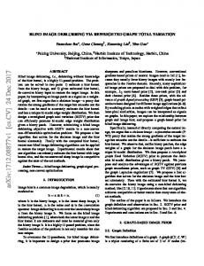
(a) Blurry image

(b) Xu & Jia[4]

(e) Krishnan et

(f) Michaeli et al.[9]

(c) Levin et al.[6] (d) Sun et al.[15]

1 0.9 0.8

Success percent

0.7 0.6 0.5 Our Cho Cho et al. Krishnan et al. Levin et al. Sun et al. Xu & Jia Michaeli & Irani

0.4 0.3 0.2 0.1

al.[17]

(g) Perrone et al.[19]

(h) Our method

Fig. 2: Visual comparisons with some state-of-the-art methods on real images with unknown kernel.

0 0

5

10

15

20

25

Error ratios

Fig. 1: Cumulative distribution of error ratios on Sun et al. dataset [15]

4.2. Qualitative Comparison on Real Images We experiment with real images which are blurred with large kernels. Fig.2 shows a comparison example with the stateof-the-art blind deconvolution methods [4, 6, 9, 15, 17, 19]. In this part, we also use the non-blind deconvolution of [18] to recover latent images. Compared with other methods, our method obtains robust blur kernels, suffers from much less ringing artifact and reveals sharper details in the recovered images.

1331

5. CONCLUSIONS In this paper, we exploit the priors on the latent image from the multi-scale structural self-similarity between cross-scale similar patches. On one hand, the prior from multi-scale similar structures is added into the latent image by means of the multi-scale nonlocal regularization according to the correspondence between multi-scale similar patches; on the other hand, the dictionary learning for sparse representation uses the down-sampled version of observed blurry image as training samples so that the sparsity of the latent image over this dictionary can be ensured. The experiments on both simulated and real blurry images show that our algorithm can effectively remove complex motion blurring from nature images.

6. REFERENCES [1] R. Fergus, B. Singh, A. Hertzmann, S. T. Roweis, and W. T. Freeman, “Removing camera shake from a single photograph,” ACM Transactions on Graphics, vol. 25, no. 3, pp. 787–794, 2006. [2] N. Joshi, R. Szeliski, and D. Kriegman, “Psf estimation using sharp edge prediction,” in IEEE Conference on Computer Vision and Pattern Recognition (CVPR), Anchorage, AK, 2008, IEEE Conference on Computer Vision and Pattern Recognition (CVPR), pp. 1–8, IEEE. [3] S. Cho and S. Lee, “Fast motion deblurring,” ACM Transactions on Graphics, vol. 28, no. 5, pp. 89–97, 2009. [4] L. Xu and J. Jia, “Two-phase kernel estimation for robust motion deblurring,” in European conference on Computer vision: Part I, Heraklion, Crete, Greece, 2010, European conference on Computer vision: Part I, pp. 157–170, Springer Berlin Heidelberg. [5] A. Levin, Y. Weiss, F. Durand, and W. T. Freeman, “Understanding and evaluating blind deconvolution algorithms,” in IEEE Conference on Computer Vision and Pattern Recognition, Miami, FL, 2009, IEEE Conference on Computer Vision and Pattern Recognition, pp. 1964–1971, IEEE. [6] A. Levin, Y. Weiss, F. Durand, and W. T. Freeman, “Efficient marginal likelihood optimization in blind deconvolution,” in IEEE Conference on Computer Vision and Pattern Recognition (CVPR), Providence, RI, 2011, IEEE Conference on Computer Vision and Pattern Recognition (CVPR), pp. 2657–2664, IEEE. [7] Q. Shan, J. Jia, and A. Agarwala, “High-quality motion deblurring from a single image,” ACM Transactions on Graphics, vol. 27, no. 3, pp. 15–19, 2008. [8] D. Perrone and P. Favaro, “Total variation blind deconvolution: The devil is in the details,” Columbus, OH, 2014, pp. 2909–2916, IEEE. [9] T. Michaeli and M. Irani, “Blind deblurring using internal patch recurrence,” in European Conference on Computer Vision., Zurich, Switzerland, 2014, European Conference on Computer Vision., pp. 783–798, Springer International Publishing. [10] M. Aharon, M. Elad, and A. Bruckstein, “Svd: An algorithm for designing overcomplete dictionaries for sparse representation,” IEEE Transactions on Signal Processing, vol. 54, no. 11, pp. 4311–4322, 2006. [11] D. Glasner, S. Bagon, and M. Irani, “Super-resolution from a single image,” in International Conference

1332

on Computer Vision, ICCV 2009, Kyoto, Japan, 2009, International Conference on Computer Vision, ICCV 2009, pp. 349–356, IEEE. [12] H. Zhang, J. Yang, Y. Zhang, and T. S. Huang, “Sparse representation based blind image deblurring,” in IEEE International Conference on Multimedia and Expo, Barcelona, Spain, 2011, IEEE International Conference on Multimedia and Expo, pp. 1–6, IEEE. [13] H. Li, Y. Zhang, H. Zhang, Y. Zhu, and J. Sun, “Blind image deblurring based on sparse prior of dictionary pair,” in International Conference on Pattern Recognition (ICPR), Tsukuba, 2012, International Conference on Pattern Recognition (ICPR), pp. 3054–3057, IEEE. [14] J. A. Tropp and A. C. Gilbert, “Signal recovery from random measurements via orthogonal matching pursuit,” IEEE Transactions on Information Theory, vol. 53, no. 12, pp. 4655–4666, 2007. [15] L. Sun, S. Cho, J. Wang, and J. Hays, “Edge-based blur kernel estimation using patch priors,” in IEEE International Conference on Computational Photography (ICCP), Cambridge, MA, 2013, IEEE International Conference on Computational Photography (ICCP), pp. 1–8, IEEE. [16] T. S. Cho, S. Paris, B. K. P. Horn, and W. T. Freeman, “Blur kernel estimation using the radon transform,” in IEEE Conference on Computer Vision and Pattern Recognition (CVPR), Providence, RI, 2011, vol. 42 of IEEE Conference on Computer Vision and Pattern Recognition (CVPR), pp. 241–248. [17] D. Krishnan, T. Tay, and R. Fergus, “Blind deconvolution using a normalized sparsity measure,” in IEEE Conference on Computer Vision and Pattern Recognition (CVPR), Providence, RI, 2011, IEEE Conference on Computer Vision and Pattern Recognition (CVPR), pp. 233–240, IEEE. [18] D. Zoran and Y. Weiss, “From learning models of natural image patches to whole image restoration,” in IEEE International Conference on Computer Vision (ICCV), Barcelona, 2011, IEEE International Conference on Computer Vision (ICCV), pp. 479–486, IEEE. [19] D. Perrone, R. Diethelm, and P. Favaro, “Blind deconvoperronediethelmperronediethelmlution via lowerbounded logarithmic image priors,” in International Conference on Energy Minimization Methods in Computer Vision and Pattern Recognition(EMMCVPR), Hong Kong, China, 2015, International Conference on Energy Minimization Methods in Computer Vision and Pattern Recognition(EMMCVPR), Springer International Publishing.