via the Viterbi algorithm, or maximum a posteriori (minimum symbol-error rate) detection via the BCJR algorithm [lo]. Such detectors offer excellent performance ...
Blind Iterative Channel .Identification and Equalization R. R. Lopes and J. R. Barry School of Electrical and Computer Engineering Georgia Institute of Technology Atlanta, GA 30332-0250 Abstract -We propose an iterative solution to the problem of blindly and jointly identifying the channel response and transmitted symbols in a digital communications system. The proposed algorithm iterates between a symbol estimator, which uses tentative channel estimates to provide soft symbol estimates, and a channel estimator, which uses the symbol estimates to improve the channel estimates. The proposed algorithm shares some similarities with the Expectation-Maximization (EM) algorithm but with lower complexity and better convergence properties. Specifically, the complexity of the proposed scheme is linear in the memory of the equalizer, and it avoids most of the local maxima that trap the EM algorithm.
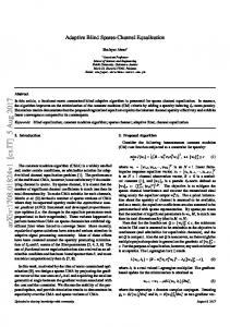
I. INTRODUCTION An important class of algorithms for blind channel identification is based on the iterative strategy depicted in Fig. I [I-91. In these algorithms, an initial channel estimate is used by a symbol estimator to provide tentative soft estimates of the transmitted symbol sequence. These estimates are used by a channel estimator to improve the channel estimates. The improved channel estimates are then used by the symbol estimator to improve the symbol estimates, and so on. Iterative techniques for channel identification have three important advantages. First, the channel estimates are capable of approaching the maximum-likelihood (ML) estimates. Second, blind identification of the channel allows the receiver to use decision-feedback equalization, ML sequence detection via the Viterbi algorithm, or maximum a posteriori (minimum symbol-error rate) detection via the BCJR algorithm [lo]. Such detectors offer excellent performance even when the channel has a spectral null, where equalizers based on linear filters (using the constant-modulus algorithm, for example)
are known to fail. Third, iterative schemes easily exploit, in a nearly optimal way, any a priori information the receiver may have about the transmitted symbols. This a priori information may arise because of pilot symbols, a training sequence, precoding, or error-control coding. Thus, iterative channel estimators are well-matched to applications involving turbo equalization [4][1 I] or semi-blind channel estimation [12]. By exploiting the existence of coding, a blind iterative detector is able to benefit from the immense coding gains that typify today's powerful codes (based on turbo coding or low-density parity-check codes, for example). These codes allow reliable communication with an SNR that is lower than ever before, which only exacerbates the identification problem for traditional algorithms that ignore the existence of coding. Most prior work in blind iterative channel identification can be tied to the EM algorithm of [13]. The first such detector [ I ] used hard decisions produced by a Viterbi sequence detector. The first use of EM with soft symbol estimates (as produced by BCJR) was proposed in [2]. It is a direct application of EM (as are [3] and [4]), and hence is guaranteed to converge to a local maximum of the joint channel-sequence likelihood function. An adaptive version [5] of EM was applied to the identification problem in [6]. The algorithms proposed in [7-91 are modifications of EM. The algorithm we propose differs from prior work in its lower complexity and improved convergence. Specifically, we propose a symbol estimator based on a DFE, whose complexity increases linearly with the equalizer memory, as opposed to exponentially with channel memory. We also propose an extended-window channel estimator which greatly reduces the probability of misconvergence to a nonglobal local maximum of the joint likelihood function.
11. PROBLEM STATEMENT
ESTIMA TOR
ESTIMATOR
Consider the transmission of K independent and identically 2 distributed zero-mean symbols ak with unit energy E[akI = 1, belonging to some alphabet A, across a dispersive channel with memory p and additive white Gaussian noise. The received signal at time k can be written as rk = h a k
Figure 1. Blind iterative channel identification.
0-7803-7097-1/01/$10.00 02001 IEEE
+ nk,
(1)
where h = (ho, hl, ..., h p ) represents the channel impulse response, a k = ( a k , a k - 1 , ..., ak-w)T and n k NO,02)is the
-
2256
noise. Let a = (ao, a l , ..., aK-l) and r = (ro, '1, ..., rN-1) denote the input and output sequences, respectively, where N = K + p. The blind channel identification problem is to estimate h and (5 relying solely on the received signal r and knowledge of the probability distribution function for a.
have access to ~52' = E [ a k l r ;h(i),6(i)]. Replacing this value in (6), and also replacing time average for ensemble average, leads to the following channel estimator:
111. EM AND BLINDCHANNEL IDENTIFICATION
for n = 0, 1, ..., p. The idea of estimating the channel by correlating the received signal with the transmitted sequence has been explored in [17], but the algorithm proposed in that work relies on a training sequence.
The EM algorithm [ 133 provides an iterative solution to the blind identification problem that fits the paradigm of Fig. 1. It generates a sequence of channel estimates with nondecreasing likelihood, and under general conditions converges to a local (not necessarily global) maximum of the likelihood function. Application to blind channel identification was first proposed in [2]. The channel estimator (see Fig. 1) for the (i + 1)-st iteration of the EM algorithm is defined by &(i+1)=
RY' c
Pi,
(2) (3)
(7)
Combing the estimates (7) into a single vector, we find that +.( 1 + 1 ) ) = p , .Thus, we may view (7) as a , .. ., h , simplification of the EM estimate RLb,;it avoids matrix inversion by replacing R, by I. This is reasonable given that R, is an a posteriori estimate of the autocorrelation matrix of the transmitted vector, which is known to be the identity. &([+I)= (j$ + I )
be an estimate As for estimating the noise variance, let of the transmitted sequence, chosen as the element of A closest to 6:) . we propose to compute 6 using:
where (4)
Since this channel estimator no longer needs Ri, the E [ a ] rh(1) ; I. symbol estimator need only produce Although the BCJR algorithm can compute U ( ' ) exactly, its high complexity (exponential in p) is often prohibitive. 3
The symbol estimator provides the values of U : ) = ..( 1 ),o -(i) E[aklr;h ( 2 ),6 (i)] and E[akak( r ;h ] that are required by (3) through (5). The symbol estimator of the EM algorithm uses the BCJR algorithm [lo], which has complexity exponential in the channel memory, and is based on the tentative channel estimates fed from the channel estimator. A
Note that Ri and p i can be viewed as estimates of the a posteriori autocorrelation matrix of the transmitted sequence and the cross-correlation vector between the transmitted and receive sequences, respectively. Thus, (2) is very similar to the least-squares solution [ 161, in which these quantities are replaced by the actual sample autocorrelation matrix and cross-correlation vector.
Iv. THE CHANNEL AND SYMBOL ESTIMATORS We first propose a low-complexity channel estimator that avoids the matrix inversion of (2). From the channel model it is clear that h, = E[rkak-,]. But
[
E[rkak-,] = E r k E [ a k - n I rkl] = E [rhE[ak-, I r]] .
We now propose a low-complexity symbol estimator based on a D E , restricting our attention to the binary alphabet A = {-I, 1 ) . Consider filtering the channel output with a minimum mean-square error DFE (MMSE-DFE), resulting i n an equalizer output Z k that is approximately free of intersymbol interference (ISI). In this case, we could write zk = A U k + u k , where A is the gain of the equivalent ISI-free channel, and the equivalent "noise" term Uk is approximately zero mean and 2 Gaussian with some variance (5, . If this model were valid, the output of the symbol estimator could be written as E[ak I rl = tanh(Azk/ot). Thus, we propose to use h'c) and 6'') to compute the MMSE-DFE coefficients, and to filter the received sequence with this equalizer. The symbol estimator then outputs tik=tanh(A.zk/o:). The complexity of this symbol estimator is independent of channel memory, and increases linearly with the length of the equalizer. 2
As for computing A and o U ,we propose that the symbol estimator be equipped with the following internal iteration:
(6)
Note that the channel estimator has no access to E[ak I rl, which requires exact channel knowledge. However, based on the iterative paradigm of Fig. 1, at the i-th iteration it does
0-7803-7097-1/01/$10.00 02001 IEEE
0
2257
(9)
which are repeated until a stop criterion is met. These iterations result from the application of the simplified channel estimator (7), (8) to a I-tap channel. Usually, only a few 2 repetitions are needed, and Aiis initialized to A0 = 0". .
V. THE EXTENDED-WINDOW ALGORITHM .
Misconvergence is a common characteristic of iterative channel identification algorithms. In fact, it is very easy to find an example in which both EM and the proposed algorithm, as defined so far, fail to identify the channel.
VI. THEIMPACT OF 6 It is interesting to note that while substituting the actual values of h or a for their estimates will always improve the performance of the iterative algorithm, the same is not true for 6. Indeed, substituting o for 6 will often result in performance degradation. Intuitively, one can think of 6 as playing two roles: in addition to measuring 6,it also acts as a nzeasure of reliability in the channel estimate h. Consider a decomposition of the observation vector:
-
To illustrate the problem of misconvergence, consider h = (20) [ l 2 3 4 51. The proposed algorithm converges to h L2.179 3.073 4.108 5.t9.2 0.1201 after 20 iterations, with K = 1000 bits, SNR = ((hl(-/02 = 20 dB, with initialization h-(O) [ l o 0 0 01 and B o , = 1, and with N f = 15 forward and Nb = 5 feedback DFE coefficients. The estimate is seen to roughly approximate a shifted or delayed version of the actual channel. This misconvergence stems from the delay mismatch between h and the initialization h"). The iterative scheme cannot compensate for this delay. In fact, after convergence, sign(&,) is a good estimate for a k - 1 , and ho can be well estimated by correlating rk with G k I . But because the delay n in (7) is limited to the narrow window (0, ..., p), (7) never computes this correlation. This observation leads us to propose the extended-window algorithm, in which (7) is computed for a broader range of n. +
To determine how much the correlation window must be extended, consider two extreme cases. First, suppose h = [l 0 0 0 ... 01 and h'z) = [O ... 0 0 0 11. In this case, the symbol estimator output &k is such that sign(Gk) = U k - p . Thus, to estimate ho we must compute (7) for n = -p. Likewise, if h = 10... 0 0 0 11 and h ( 2 ) = [ l 0 0 0 ... 01, the symbol estimator output iik is such that sign(&,,) = U k + p, and so to estimate h p we must compute (7) for n = 2p. These observations suggest the extended-window algorithm, which computes
for n E {-p,..., 2p). By doing this, we ensure that g = i&, ...,g2,1 has p + 1 entries that estimate the desired correlations E[rkak,], for n E (0, .... p). Its remaining terms are an estimate of E[rk~k-~I for n P (0, ..., p), and hence should be close to zero. We may thus define the channel estimate by jJl+l) = I&, . .., gv+ ,I, where the delay parameter v E (-p,..., p] is chosen so that h(i+l)represents the p + 1 consecutive coefficients of g with highest energy. The noise variance may again be estimated using (8), but accounting for the delay v by using cik = sign(&:!, 1.
0-7803-7097-1/01/$10.00 02001 IEEE
r = a * h + a * (h - h) + n,
(12)
where * denotes convolution. The second term represents the contribution to r from the estimation error. By using h to model the channel in the BCJR algorithm, we are in effect lumping the estimation error with the noise. Combining the two results in an effective noise sequence with variance larger than 02. It is thus appropriate that 6 should exceed 0 whenever h differs from h. Alternatively, it stands to reason that an unreliable channel estimate should translate to an unreliable (i.e., with small magnitude) symbol estimate, regardless of how well a * h matches r. A large value of 6 in BCJR ensures this. Fortunately, (8) measures the energy of both the second and the third term in ( I 2 ) . If h is a poor channel estimate, U will also be a poor estimate for a,and convolving U and h will produce a poor match for r. Thus, (8) will produce a large estimated noise variance. An interesting and natural question is if the B produced by (8) is large enough. We will show in the next section that increasing 6 beyond (8) helps avoid misconvergence.
VII. SIMULATION RESULTS As a first test of the extended-window algorithm, we have simulated the transmission of K = 1000 bits over the channel h = [-0.2287, 0.3964, 0.7623, 0.3964, -0.22871 from [7], with SNR = 18 dB, N f = 15 forward and Nb = 5 feedback DFE coefficients, and 3 inner iterations. To stress the fact that the proposed algorithm is not sensitive to initial conditions, we initialized h randomly using h(O) = u 6 (o)/ llull , where U N(0, I) and 6& = C r l i r i / 2 N . (This implies an initial estimated SNR of 0 dB.). The curves shown in Fig. 2 are the average of 100 independent runs of this experiment. Only the convergence of h0 , h2 and h3 is shown. (The behavior of h1 and is similar to that of hg and ho, respectively, but we show only those with worse convergence.) The shaded regions around the channel estimates correspond to plus and minus one standard deviation. For comparison, we show the average behavior of the EM algorithm in Fig. 3 . Unlike the good
-
2258
performance of the extended window algorithm, the EM algorithm even fails to converge in the mean to the correct estimates. This happens because the EM algorithm can get trapped in local maxima of the likelihood function [ 131, while the extended-window does not. To further support the claim that the proposed algorithm avoids most of the local maxima of the likelihood function that trap the EM algorithm, we ran both these algorithms on 1,000 random channels of memory p = 4, generated as h = U / llull , where U - N(0, I). The estimates were initialized to 6& - Xf;d r i / 2 N and h(O) = , 0, ..., 01. We used SNR = 18 dB, K = 1000 bits, N f = 40, Nb = 10, and 3 inner iterations. In Fig. 4 we show the rate of success of the algorithms versus iteration. The algorithms were deemed successful if they produced fewer than 3 bit errors in a block. It is again clear that the extended-window algorithm has a much better
performance than the EM algorithm. This can also be seen in Fig. 5 , where we show histograms of the norm of the estimation errors (the difference between the channel vector and its estimate) for the extended-window and the EM algorithms, computed after 70 iterations. We see that while the proposed algorithm produces a negligible number of errors with norm above 0.2, about 45% of the errors produced by the EM algorithm have norm above 0.2. Some interesting observations can be made by considering the unsuccessful runs of the extended-window algorithm. Consider, for instance, h = L0.4823, 0.0194, -0.5889, 0.6285, -0.15861, which was not correctly estimated in the previous experiment. First note that this channel does not present severe ISI. In fact, none of the channels the algorithm failed to identify introduce severe ISI. Instead, their common characteristic is the presence of 3 or more coefficients of 100 90 80 70 60 U
a, U ;ti
50
U)
$
40
U
30 20 10
0
0
30
20
10
10
20
30
50
60
70
Figure 4. Success rate for extended window and EM algorithms for random channels over an ensemble of 1000.
Figure 2. Estimates of h = [-0.2287, 0.3964, 0.7623, 0.3964, 0.22871, produced by the extended-window algorithm.
-
fi* .................................................
0.8
40
Iteration
ITERATION
400
2
0.6 0.4
0.2 150 0
100
-0.2
50
'
'"U
-0.4l
0
I
I
I
I
I
I
I
10
I
I
I
20
0
I
0
30
IEEE
0.2
0.3
0.4
0.5
0.6
0.7
0.8
0.9
Figure 5. Histograms of estimation errors for the extendedwindow and the EM algorithms.
Figure 3. EM estimates of same channel as Fig. 2.
0-7803-7097-1/01/$10.00 02001
0.1
Norm of Estimation Error
ITERATION
2259
approximately the same magnitude. The convergence behavior is also a strong function of the transmitted block length K. For this particular channel, with SNR = 18 dB, K = 1887 bits, N f = 40, Nb = 10, and 3 inner iterations, the proposed algorithm fails, yielding BER = 30% after convergence. If K is changed to K = 1888, then the algorithm is successful, yielding no errors after convergence. Thus, for this particular channel and others we have tested, there is a cutoff block length K above which the algorithm is successful, and below which the algorithm fails. The impact of 6 was also analyzed. For h =[0.4823, 0.0194, -0.5889, 0.6285, -0.15861, K = 1000, SNR = 13 dB, IVf = 40,Nb = 10, 3 inner iterations, and with 6 computed according to (8), the proposed algorithm fails, yielding BER = 30% after convergence. However, if we pass a6 to the symbol estimator instead of 6 , then a suitable choice for a can lead to successful convergence. In Fig. 6, we plot the BER after 60 iterations versus a. We see that increasing c( can improve the performance of the algorithm, but increasing it too much will again cause the algorithm to fail. In spite of this encouraging observation, we were not able to find a strategy that significantly impacts the success rate over a broad range of channels. For instance, keeping a = 3 and rerunning the experiment with the 1000 random channels, we obtained a success rate of 95.6%, as opposed to 95.3% obtained with the regular algorithm (a = 1). Thus, finding the optimal value for a for a broad class of channels remains an open problem.
VIII. CONCLUSIONS We presented an iterative channel identification technique with complexity linear in the number of channel coefficients. We have shown that this technique can be seen as a reducedcomplexity version of the EM algorithm. A key feature of the proposed algorithm is its extended window, which greatly improves the convergence behavior of the algorithm, avoiding most of the local maxima of the likelihood function that trap the EM algorithm. A small percentage of channels still cause difficulty, but a smarter initialization strategy (as opposed to the identity initialization proposed here) will likely help. Nevertheless, the problem of devising an iterative strategy that is guaranteed to always avoid misconvergence, regardless of initialization, remains open.
C. Anton-Haro, J . A. R. Fonollosa and J . R. Fonollosa. “Blind Channel Estimation and Data Detection Using Hidden Markov Models.” lEEE Trans. Si,-. Proc.. vol. 4.5, no. I , pp. 24 1-246. Jan 1997.
J. Garcia-Frias and J. D. Villasenor, “Blind Turbo Decoding and Equalization,” IEEE VeIiic. Techti. Conference, vol. 3, pp. I88 I - 1885, 1999. V. Krishnamurthy, J . B. Moore. “On-Line Estimation of Hidden Markov Model Parameters Based on the Kullback-Leibler Information Measure,’’ E E E Tram. Sig. Pmc., vol. 41, no. 8, pp. 2557-2573, Aug 1993. L. B. White. S. Perreau, P. Duhamel, “Reduced Complexity Blind Equalization for FIR Channel Input Markov Models”, IEEE hrertiutionul Conference on Cotn~nu~~icutions. vol. 2, pp.993-997, 1995. M. Shao and C. L. Nikias, “An MUMMSE Estimation Approach to blind Equalization”. /CASSE vol. 4. pp. 569-572, 1994. H. A. Cirpan and M. K. Tsatsanis, “Stochastic Maximum Likelihood Methods for Semi-Blind Channel Equalization,” Sigiiul Processirrg Lerrers, vol. 5, no. I , pp. 1629-1632, Jan 1998. B. P. Paris. “Self-Adaptive Maximum-Likelihood Sequence Estimation,” IEEE Global Te/econltJiufiicatinollsCol$, vol. 4, pp. 92-96, 1993. [IO] L. R. Bahl, J. Cocke, E Jelinek, and J. Raviv, “Optimal Decoding of Linear Codes for Minimizing Symbol Error Rate,” IEEE Trurns. 011 It@ T/ieoty, pp. 284-287, March 1974. [ I I ] C. Douillard, M. Jezequel. C. Berrou, A. Picart, P. Didier, A. Glavieux, “Iterative Correction of Intersymbol Interference: Turbo Equalization,” Ectropeari Trans. Telecom, vol. 6,110.5,pp.507-51 I . Sept.-Oct. 1995. [I21 J. Ayadi, E. de Carvalho and D. T. M. Slock, “Blind and Semi-Blind Maximum Likelihood Methods for FIR Multichannel Identification,” IEEEICASSP, vol. 6, pp. 3185 -3188, 1998. [13] A. P. Dempster. N. M. Laird and D. B. Rubin, “Maximum Likelihood from Incomplete Data Via the EM Algorithm”, J o i r n i d of the Royal Stutisrics Societ): vol. 39, no. 1 , pp 1-38, 1997. [14] C. Berrou, A. Glavieux. and P. Thitimajshima. “Near Shannon Limit Error-Correcting Coding and Decoding: Turbo Codes( I),” f E E E Inrern. Cor$ on Conzmr~r~icurioris, pp. 1064-70, Geneva, May 1993. [ 151 M. Varanasi and B. Aazhang, “Multistage Detection in Asynchronous Code-Division Multiple-Access Communications,” IEEE Truriscrcfiotu on Cn,nmia,icutiorzs, vol. 38, pp. 509-519, April 1990. [ 161 Poor, H . V.,AJI Iurroducrion ro Sipicr[ Detecriori und Esrirnuriori, Second Edition, Springer-Verlag. 1994. [I71 C. A. Montemayor, P. K. Flikkema, “Near-Optimum Iterative Estimation of Dispersive Multipath Channels,” IEEE Velzicitlur Technology Conference, vol. 3, pp. 2246-2250, 1998.
11111111
IX. REFERENCES [I ]
[2]
M. Feder and J. A. Catipovic. “Algorithms for Joint Channel Estimation and Data Recovery - Application to Equalization in Underwater Conimunications.” IEEE J. Oceanic EJZQ,vol. 16, no. 1, pp. 42-5. Jan. 199I . G . K. Kaleh and R. Vallet, “Joint Parameter Estimation and Symbol Detection for Linear or Nonlinear Unknown Channels”, IEEE Transactiom 011 CorJlnictriicatiofis.vol. 42, no. 7, pp. 2406-241 3. July 1994.
0.001 1
I
I
t
I
I
I
2
3
4
5
6
7
NOISE AMPLIFICATION FACTOR
a
Figure 6. Fixing 6 artificially high improves performance
0-7803-7097-1/01/$10.00 02001 IEEE
2260