IEEE SIGNAL PROCESSING LETTERS, VOL. 20, NO. 7, JULY 2013
653
Blind System Identification Using Sparse Learning for TDOA Estimation of Room Reflections Konrad Kowalczyk, Emanuël A. P. Habets, Senior Member, IEEE, Walter Kellermann, Fellow, IEEE, and Patrick A. Naylor, Senior Member, IEEE
Abstract—Localization of early room reflections can be achieved by estimating the time-differences-of-arrival (TDOAs) of reflected waves between elements of a microphone array. For an unknown source, we propose to apply sparse blind system identification (BSI) methods to identify the acoustic impulse responses, from which the TDOAs of temporally sparse reflections are estimated. The proposed time- and frequency-domain adaptive algorithms based on crossrelation formulation are regularized by incorporating an -norm sparseness constraint, which is realized using a split Bregman method. These algorithms are shown to outperform standard crossrelation-based BSI techniques when estimating TDOAs of reflections in the presence of background noise. Index Terms—Blind system identification, Bregman method, crossrelation error, sparse learning, time delay estimation.
I. INTRODUCTION NFORMATION about the directions of arrival of the source signal and room reflections can be applied to improve the performance of several audio applications, such as signal enhancement [1] and room-compensated audio reproduction [2]. Typically the time-difference-of-arrival (TDOA) of the direct path is estimated with the aim to localize a speaker or an interfering sound source, see [3] for an overview of available techniques. Recently reflection localization has gained more interest in the context of inferring room geometry [4] and room-aware sound reproduction [2]. Localization of reflections can be performed using the TDOAs of the reflected waves between different microphone signals, which can be conveniently computed from (blindly) estimated acoustic impulse responses (AIRs). In particular, the crossrelation-based single-input multiple-output (SIMO) blind system identification (BSI), which exploits spatial differences between multiple microphone signals, has received significant attention as it does not require any assumption about the source signal and can be formulated as an adaptive algorithm [5], [6]. Furthermore, adaptive BSI algorithms have been shown
I
Manuscript received March 25, 2013; revised April 29, 2013; accepted April 29, 2013. Date of publication May 01, 2013; date of current version May 17, 2013. The associate editor coordinating the review of this manuscript and approving it for publication was Prof. Augusto Sarti. K. Kowalczyk and E. A. P. Habets are with the International Audio Laboratories Erlangen (a joint institution between the University of Erlangen-Nuremberg and Audio Department, Fraunhofer IIS), 91058 Erlangen, Germany (e-mail:
[email protected];
[email protected]) W. Kellermann is with the Chair of Multimedia Communication and Signal Processing (LMS), University of Erlangen-Nuremberg, 91058 Erlangen, Germany (e-mail:
[email protected]). P. A. Naylor is with the Department of Electrical and Electronic Engineering, Imperial College London, South Kensington Campus, London SW7 2AZ, U.K. (e-mail:
[email protected]). Color versions of one or more of the figures in this paper are available online at http://ieeexplore.ieee.org. Digital Object Identifier 10.1109/LSP.2013.2261059
in [3] to outperform crosscorrelation-based techniques, such as generalized crosscorrelation (GCC), for source localization in noisy and reverberant environments. As the power of the direct-path signal is typically higher than the power of the early reflections, the estimation of the latter becomes more challenging, especially in the presence of additional noise. In this letter, we aim to increase the robustness to noise of BSI methods for TDOA estimation of room reflections by incorporating a sparse AIR model. The -regularized crossrelation formulation is obtained by means of a split Bregman iteration method [7], [8], which is known to be robust to background noise. The presented sparse BSI problem formulation is advantageous since the early part of acoustic impulse responses has a sparse structure [9] so that for TDOA estimation of most significant reflections only the knowledge of sparse AIR components is needed. Sparse BSI has also been applied to speech extraction [10] and dereverberation [11]. This letter presents a method to formulate adaptive BSI algorithms with sparse learning that operate in time and frequency domains. In particular, two algorithms are derived by extending the multichannel least mean squares (MCLMS) [5] and the normalized multichannel frequency-domain LMS (NMCFLMS) [6] algorithms to sparse BSI. Other algorithms can be derived analogously. II. PROBLEM FORMULATION In the assumed reverberation model, the th microphone signal of a -element microphone array is given by (1) where is the original unknown source signal, denotes the spatially white background noise, and denotes the th impulse response of length , which can be linearly decomposed into (2) where and model the fractional propagation time delays and attenuation factors of the direct-path signal and early room reflections , respectively, and denotes the filter that models late reverberation. In this work, we aim to estimate the TDOA of the th room reflection between the th and th microphone. Such a TDOA is defined as (3) and denote the estimated time delays of reflecwhere tion . Note that the task of matching the peaks between different AIRs corresponding to the same reflection [4] is beyond the scope of this letter.
1070-9908/$31.00 © 2013 IEEE
654
IEEE SIGNAL PROCESSING LETTERS, VOL. 20, NO. 7, JULY 2013
III. BLIND SPARSE SYSTEM IDENTIFICATION To find sparse solutions of an unknown system, -norm regularization can be incorporated into the generic BSI cost function , which can be formulated as the following constrained problem
solved using iterative minimization techniques with respect to and , respectively, i.e.,
(11a) (11b)
(4) where , are the estimates of AIRs, and ensures that trivial , are avoided. Such a generic zero solutions, i.e., BSI cost function is given by [5] (5) with the a priori error defined as a sum of crossrelation errors for each microphone pair ( , ) (6) whereas the
with the unit-norm constraint explicitly written in (11a). IV. ADAPTIVE BSI WITH SPARSE LEARNING An adaptive BSI algorithm using sparse learning can be realized by iteratively solving (11a), (11b), and (10b), respectively. The first optimization problem (11a) is differentiable and therefore can be solved using an adaptive gradient-based algorithm. In this letter, we extend two adaptive BSI algorithms, namely, the multichannel least mean squares (MCLMS) [5] and the normalized multichannel frequency-domain LMS (NMCFLMS) [6] algorithms by incorporating an -norm regularization. A. Sparse Multichannel Least Mean Squares Algorithm Let us replace the iteration index with the time index denote the th microphone signal vector at as
-norm sparseness cost function is given by (7)
where the uniform regularization parameter defines the relation between the sum of pairwise squares of the crossrelation errors and the sparseness of blindly identified AIRs. Solving (4) using an adaptive algorithm requires calculating higher-order moments (at least the first-order gradient) of the cost function . Both and are convex functions but is non-differentiable and therefore (4) cannot be solved directly. In order to formulate an adaptive algorithm, the - and -norm components need to be decoupled. For convenience of derivations, let us first omit the unit-norm constraint and reformulate (4) as
and (12)
1) Adaptive Sparse Crossrelation-Based Update: The sparse MCLMS (SMCLMS) update is obtained by taking the gradient of the cost function given by (11a), i.e.,
(13) which after setting can be expressed as
and taking the respective derivatives
(8) any linear operator, and is an auxiliary variable vector with elements . Equation (8) can be further reformulated into an unconstrained optimization problem using a quadratic penalty function as where
denotes
(9) where is a Lagrange multiplier. The split Bregman iteration method [7] can then be applied such that a set of unconstrained problems and Bregman updates is obtained, which is given by
(10a) (10b) where , denotes the so-called Bregman variable vector, and is an iteration index. Note that this way the error introduced by the constraint is added back in the Bregman update (10b), which makes this technique particularly robust against noise. Since is convex but non-differentiable, (10a) can finally be split into the - and -norm components which can be
(14) by normalizing the AIR Enforcing the unit constraint estimate at each iteration , we obtain
(15) where is the step size, the sum of squares of crossrelation is given by (6), and is a matrix with errors ): crossrelation matrices as elements ( e.g.,
.. .
.. .
..
.
.. .
(16)
2) Updating Auxiliary and Bregman Variables: Having solved the minimization problem in (11a) using (15) at each , we can reduce the computational complexity of the algorithm by updating (11b) and (10b) only every samples, i.e., only . First note at those time instances when
KOWALCZYK et al.: BLIND SYSTEM IDENTIFICATION USING SPARSE LEARNING
that the cost function in (11b) exhibits no coupling between the elements of , thus the optimum value of for (11b) can be conveniently calculated using the so-called shrinkage operator [7]. For , this optimum solution is given by (17) where denotes the floor operator, and the shrinkage operator is applied to compute each element of separately:
(18) and . In the final step, the for samples: Bregman update needs to be performed every (19) For clarity of presentation, the consecutive processing steps of the SMCLMS algorithm are summarized as Algorithm 1.
,
matrix. Note that the length of the block is selected as with an overlap of 50%, and the th block of the th microphone signal is given by (23) A diagonal matrix with diagonal elements given by the DFT is denoted with , and the frequency-domain of crossrelation error is given by [6]
(24) with the window matrices , , and and . In the second step, the solution (21) is transformed back to the time domain, and -regularization is introduced as
(25) which after normalizing the AIR estimates yields the following final update rule for the sparse NMCFLMS algorithm:
Algorithm 1 SMCLMS initialize:
655
,
do Calculate (16) and (6) with (12) for Calculate (15) if then Calculate (17) Calculate (19) end if
(26)
while th input sample exists
B. Sparse Normalized Multichannel Frequency-Domain LMS Algorithm In the following, we present a frequency-domain -norm regularized BSI algorithm. Note that the -norm regularization is a time-domain phenomenon, since we search for solutions which are sparse in time. Therefore, to develop the frequency-domain formulation of (11a), we can first calculate a nonsparse solution in the frequency domain, i.e, (20) and the -regularization is accounted for after transforming the solution of (20) back to the time domain. Thus the standard NMCFLMS computations are performed first according to [6]
for all channels and the 50% where overlap-save is realized using a window matrix . Further two steps include computing the auxiliary and Bregman variables using the following relations (27) (28) For clarity, the processing steps of the full SNMCFLMS algorithm are summarized as Algorithm 2. Algorithm 2 SNMCFLMS initialize: , , do Calculate (24), (22), and (21) with (23) for Calculate (26) for Calculate (27) Calculate (28) while
(21) (22) is the block index, denotes the where forgetting factor, is the regularization parameter, is the th AIR estimate with zero padding, and all frequency-domain values are generally denoted with an underscore, e.g., , where is an DFT
th block of input samples exists
V. PERFORMANCE EVALUATION The TDOA estimation performance of the proposed sparse algorithms was compared to standard (non-sparse) counterparts through a set of 50 Monte Carlo simulations. In the experiments, a 15 s duration white Gaussian noise was used as a source signal, which was captured using 2- and 4-element uniform linear arrays (with microphone spacing ) positioned near the center of a 5 6.3 3 m room simulated using the image-source method. The source was located at
656
IEEE SIGNAL PROCESSING LETTERS, VOL. 20, NO. 7, JULY 2013
Fig. 1. TDOA error as a function of time (after initial convergence of 0.6 s) for and . SNMCFLMS and NMCFLMS; TABLE I RMS TDOA ERROR IN SAMPLES (TOP PANEL) AND THE CORRESPONDING DOA ERROR IN DEGREES (BOTTOM PANEL)
Fig. 2. Acoustic impulse responses for and : a) nor; b) AIR estimated using NMCFLMS; c) AIR malized simulated AIR for estimated using SNMCFLMS.
(1.75,0.05,2) m and the reflection coefficient was set to 0.82 for all walls, resulting in a reverberation time of 360 ms. For the SMCLMS algorithm, the following parameters were set: kHz, AIR filter length , and , whereas for the SNMCFLMS algorithm, experiments were performed for kHz, , , , and . The sparseness parameters of SMCLMS were determined empirically: and for (and was increased by a factor for lower SNRs). The and parameters of SNMCFLMS were set to for (and we set for lower SNR to emphasize the sparseness constraint). The (in samples) between root mean square TDOA error the peaks of simulated and estimated AIRs for the direct-path and 6 first-order reflections for all microphone pairs, was used as a performance measure for different SNR values. The corresponding direction of arrival (DOA) error, calculated as , where is the wave speed, is also provided. Note that the peak matching between AIRs was resolved by the AIR simulator, and the DOA errors increase with decreasing microphone spacing and sampling frequency. The results for both experiments are presented in Table I; the TDOA error as a function of time for one scenario is depicted in Fig. 1. As can be observed, sparse algorithms in general lead to a smaller TDOA estimation error. In particular, they are significantly better at low SNR, where the AIRs estimated with nonsparse algorithms become very noisy, and eventually the reflection peaks cannot be found in such estimates (see Table I and Fig. 2). VI. CONCLUSIONS This letter presents a method for crossrelation-based blind identification of sparse systems for accurate TDOA estimation
of early room reflections. Two adaptive time- and frequency-domain algorithms are proposed, where -norm regularization is incorporated into the BSI formulation using a split Bregman method; in principle, other sparse BSI algorithms can be formulated in a similar fashion. The proposed methods are shown to outperform their non-sparse counterparts, particularly so in noisy acoustic conditions, and enable the robust performance even at very low SNR, which cannot be otherwise achieved. REFERENCES [1] Y. Peled and B. Rafaely, “Method for dereverberation and noise reduction using spherical microphone arrays,” in Proc. IEEE Int. Conf. Acoust., Speech and Signal Process. (ICASSP), Mar. 2010, pp. 113–116. [2] T. Betlehem and T. Abhayapala, “Theory and design of sound field reproduction in reverberant rooms,” J. Acoust. Soc. Amer., vol. 117, pp. 2100–2111, 2005. [3] J. Chen, J. Benesty, and Y. Huang, “Time delay estimation in room acoustic environments: An overview,” EURASIP J. Appl. Signal Process., vol. Special issue on advances in multimicrophone speech processing, pp. 1–19, 2006. [4] F. Antonacci, J. Filos, M. Thomas, E. Habets, A. Sarti, P. Naylor, and S. Tubaro, “Inference of room geometry from acoustic impulse responses,” IEEE Trans. Audio, Speech, Lang. Process., vol. 20, no. 10, pp. 2683–2695, Dec. 2012. [5] Y. Huang and J. Benesty, “Adaptive multi-channel least mean square and Newton algorithms for blind channel identification,” Signal Process., vol. 82, pp. 1127–1138, Aug. 2002. [6] Y. Huang and J. Benesty, “A class of frequency-domain adaptive approaches to blind multichannel identification,” IEEE Trans. Signal Process., vol. 51, no. 1, pp. 11–24, Jan. 2003. [7] T. Goldstein and S. Osher, “The split Bregman algorithm for L1 regularized problems,” SIAM J. Imag. Sci., vol. 2, no. 2, pp. 323–343, 2009. [8] Y. Wang, W. Yin, and Y. Zhang, “A Fast Algorithm for Image Deblurring with Total Variation Regularization,” Tech. Rep., CAAM, 2007. [9] K. Wagner and M. Doroslovacki, “Towards analytical convergence analysis of proportionate-type NLMS algorithms,” in Proc. IEEE Int. Conf. Acoust., Speech and Signal Process. (ICASSP), Apr. 2008, pp. 3825–3828. [10] M. Yu, W. Ma, J. Xin, and S. Osher, “Multi-channel l1 regularized convex speech enhancement model and fast computation by the split Bregman method,” IEEE Trans. Audio, Speech, Lang. Process., vol. 20, no. 2, pp. 661–675, Feb. 2012. [11] Y. Lin, J. Chen, Y. Kim, and D. Lee, “Blind channel identification for speech dereverberation using l1-norm sparse learning,” in Neural Inform. Process. Syst. (NIPS), 2007.