Bloom Filters in Probabilistic Verification - Semantic Scholar

Bloom Filters in Probabilistic Verification Peter C. Dillinger and Panagiotis Manolios Georgia Institute of Technology College of Computing, CERCS 801 Atlantic Drive Atlanta, GA 30332-0280 {peterd,manolios}@cc.gatech.edu

Abstract. Probabilistic techniques for verification of finite-state transition systems offer huge memory savings over deterministic techniques. The two leading probabilistic schemes are hash compaction and the bitstate method, which stores states in a Bloom filter. Bloom filters have been criticized for being slow, inaccurate, and memory-inefficient, but in this paper, we show how to obtain Bloom filters that are simultaneously fast, accurate, memory-efficient, scalable, and flexible. The idea is that we can introduce large dependences among the hash functions of a Bloom filter with almost no observable effect on accuracy, and because computation of independent hash functions was the dominant computational cost of accurate Bloom filters and model checkers based on them, our savings are tremendous. We present a mathematical analysis of Bloom filters in verification in unprecedented detail, which enables us to give a fresh comparison between hash compaction and Bloom filters. Finally, we validate our work and analyses with extensive testing using 3SPIN, a model checker we developed by extending SPIN.

1 Introduction Despite its simplicity, explicit-state model checking has proved to be an effective verification technique and has led to numerous tools, including SPIN [14], Murϕ [18], TLC [23], Java PathFinder [20], etc. The state explosion problem is especially acute in explicit-state model checking because the amount of memory required depends linearly on the number of reachable states, which is often too large to enumerate in main memory. Disk can be utilized intelligently [17, 23], but such algorithms will probably continue to be outperformed by algorithms that take advantage of the fast random access time of main memory. Storing states more compactly in memory, therefore, is very desirable, and because of the huge memory savings available, storing states in a probabilistic data structure has become a popular approach and the topic of significant research. Virtually all of the proposed probabilistic verification approaches utilize one of two data structures: a Bloom filter [14] or a compacted hash table [18]. The Bloom filter, dating back to 1970 [1], is the data structure underlying “supertrace” [12], “multihashing” [21], and “bitstate hashing” [13]. Compacted hash tables are utilized by “hashcompact” [21] and the first version of “hash compaction” [18], but the technique was not perfected until [19].

2

P. C. Dillinger and P. Manolios

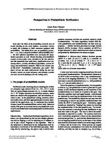
The literature contains explanations on both sides of the Bloom filter vs. hash compaction debate as to why each data structure is the best. We have found that neither is best, but that there are scenarios under which each is the best choice. More specifically, we identify three probabilistic verification techniques (based on the two data structures), each of which we believe is the best choice for some level of knowledge of the state space size. When the state space size is completely unknown, Holzmann’s supertrace method, which uses a Bloom filter with two hash functions, is the best choice because of its high expected coverage over a wide range of state space sizes (Figure 1, right graph). Supertrace is fast but starts omitting states for state spaces much smaller than other approaches (see Figure 1, left graph). Nevertheless, we can estimate actual state space sizes rather accurately with supertrace (see Section 3.3). When we know the size of the state space rather accurately—if we have an estimate that we are reasonably certain is within about 15% of the actual size—the best choice is a compacted hash table configured with slightly more cells than the maximum estimated state space size. This technique gives exceptionally high accuracy within this narrow range of state space sizes (Figure 1, left graph), and its speed is similar to supertrace’s. If, however, the data structure overflows (right graph) or is underpopulated (left graph), a Bloom filter configured for the same estimate would have been a better choice. When we have a rough estimate of the state space size, a Bloom filter configured for that estimate can tolerate much more deviation from the estimate than hash compaction can, and is likely to be much more accurate than supertrace. Such a configuration remains a respectable choice even if the estimate is off by a factor of five or more. This last technique usually calls for a Bloom filter with many more hash functions than supertrace’s two, but until our improvements to Bloom filters, introduced in [5], such configurations were unreasonably slow and not considered a good choice: “In a well-tuned model checker, the run-time requirements of the search depend linearly on [the number of hash functions]: computing hash functions is the single most expensive operation a model checker must perform” [14]. “[C]omputing 20 hash functions is quite expensive and will substantially slow down the search. Hash compaction is also superior in this regard, requiring only one 96-bit signature to be calculated” [22]. Our improvements, which require only a 2-3 word signature to be computed on the state descriptor, nullify these claims and make the configured Bloom filter technique a good choice for the rough estimate case. If supertrace provides an estimate of state space size sufficient for configuring hash compaction, when do we have a only a rough estimate of the state space size? One will have a rough estimate at many times during the development and verification of a model. First of all, small changes to a model during development can easily modify the size of a state space by more than 15%. Secondly, most models are parameterized and the state space sizes of larger instances can only be predicted roughly with respect to smaller instances. Because of its reasonable handling of a wide range of state space sizes, the Bloom filter is preferable in these cases. Version 2.0 of 3SPIN, our modified version of the SPIN model checker, is designed around the three probabilistic verification modes described above. Whenever 3SPIN finishes a verification run that revealed no errors in the model, it outputs detailed information on the expected accuracy of the run, uses this information to output an esti-

Bloom Filters in Probabilistic Verification

3

80

0.1

% of states omitted

probability of any omissions

100 1

0.01 0.001 0.0001 1e-05

Hash compaction Bloom filter Supertrace

1e-06 3.16228e+07 1e+08 3.16228e+08 Actual size of state space (log scale)

Hash compaction Bloom filter Supertrace

60 40 20 0 3.16228e+07 1e+08 3.16228e+08 Actual size of state space (log scale)

Fig. 1. These graphs show the accuracy of three probabilistic verification techniques/configurations for various state space sizes. In both graphs, lower is better. The data points for “Hash compaction” and “Bloom filter” are obtained with data structures optimized for a state space size of 108 , using 400MB of memory. The graphs show the accuracy of the data structures as the size of the state space varies. The left graph shows the probability that even a single omission occurs, while the right graphs shows the expected percentage of states omitted. The “Bloom filter” (k = 24) and “Supertrace” (k = 2) accuracies are computed using the analyses in Section 3. To compute the “Hash compaction” values we need to know the number of expected collisions in the table for the verifier run represented by each data point [18]. We determine this experimentally by counting the number of collisions in 3SPIN’s ordered, compacted table implementation, which in this case uses 32 bits per state and has a maximum visitable size of 104857589.

mate of the actual state space size, and recommends bitstate or hashcompact configurations for future runs. We used various versions and configurations of 3SPIN for the experimental results in this paper, but 3SPIN always seeds its hash functions based on the current time, resulting in virtually independent functions among executions. Unless otherwise specified, timings are taken on a 2.2Ghz non-Xeon Pentium4 (Dell Precision 340), with 512MB PC800 RDRAM running Red Hat Linux 9 with the 2.4.20 kernel. We used version 3.1.1 of the GNU C compiler with the following arguments: -O3 march=pentium3 -mcpu=pentium4. One category of related work is state space caching and the t-limited scheme of hash compaction [19]. This approach offers more flexibility to hash-compacted tables and might be a reasonable choice if memory is so constrained that a hash-compacted table of the whole state space is too inaccurate, but we don’t see this scheme as a viable replacement for the Bloom filter. Unlike state space caching, supertrace is able to explore a huge number of states with no redundant work, allowing it to find errors quickly. Another problem with state-space caching is that it does not give an indication of the size of the state space. This is acceptable in cases where state-space caching is a good choice for the problem size, but trying state-space caching is not a good way to test whether it is a good solution, because it is difficult to distinguish a process that is about to finish from one that will do many times more work than a Bloom filter. Another category of related work is reductions that can play their own role in tackling state explosion. Both symmetry [3, 7, 6] and partial-order reductions [9, 11] are compatible with the probabilistic techniques discussed. 3SPIN preserves SPIN’s partial-

4


order compatibility, but we have disabled it in our tests in order to more accurately measure accuracy and to work with larger state spaces. This paper examines Bloom filters for verification in unprecedented detail and gives analytical and empirical validation of the speed and accuracy of our improved Bloom filters. Section 2 introduces Bloom filters and reviews basic analyses that, until now, have not been fully utilized by the verification community. Section 3 extends these analyses by presenting two accuracy metrics for evaluating the performance of Bloom filters as visited lists. Section 4 details the effects of sacrificing hash function independence. Section 5 describes replacements for independent hash functions that represent various tradeoffs in efficiency and accuracy, though all our techniques provide huge speed benefits at virtually unobservable accuracy costs. Section 6 gives the results of many tests with modified versions of the SPIN model checker. The results validate our analytical accuracy claims. We end by concisely restating our contributions in Section 7.

2 Bloom Filters A Bloom filter is used to represent subsets of some universe U. A Bloom filter is implemented as an array of m bits, uses k index functions mapping elements in U to [0..m), and supports two basic operations: add and query. The index functions are traditionally assumed to be hash functions with the standard assumptions that they are random, uniform, and independent, though these assumptions can be replaced with universal hashing arguments. Initially, all bits in the Bloom filter are set to 0. To add u ∈ U to a Bloom filter, the index functions are used to generate k indices into the array and the corresponding bits are set to 1. A query is positive iff all k referenced bits are 1. A negative query clearly indicates that the element is not in the Bloom filter, but a positive query may be due to a false positive, the case in which the queried element was not added to the Bloom filter, but all k queried bits are 1 (due to other additions). We now analyze the probability of a single query of an unadded element returning a false positive (taken from [2]). Note that if p is the probability that a random bit of the Bloom filter is 1, then the probability of a false positive is pk , the probability that all k index functions map to a 1. If we let i be the number of elements that have been added to the Bloom filter, then p = 1 − (1 − m1 )ik , as ik bits were randomly selected, BF to denote the with probability m1 , in the process of adding i elements. We use f m,k,i probability that the (i + 1)st addition causes a false positive. This construction of the false positive probability is far more accurate than the analyses of bitstate hashing that appear in verification literature [21, 13, 22]. These analyses assumed that every addition to the data structure flips k 00 s to 10 s. This assumption is far from reasonable, e.g., when the data structure contains half 1’s and half 0’s, the expected number of 0’s that are flipped by an addition is 2k . This property is crucial to the flexibility of Bloom filters and is necessary for accurate analysis. The false positive probability is obviously an important metric, and with some work m −1 ) . In [2], the term (1 − one can show that it is minimized exactly when k = (i log2 m−1 ik

is approximated by e− m , and the claim is made that, modulo this approximation, the probability of false positives is minimized when k = mi ln 2, where ln is loge . One can show that this last formula is an upper approximation. 1 ik m)


5

3 Bloom Filters in Verification Although perfect for some applications [16, 8], the false positive rate is insufficient as a metric for evaluating the accuracy of Bloom filters in probabilistic explicit-state model checking. More appropriate metrics are based on the number of states that are omitted from the search, which tells us how much uncertainty there is in the model checking result. The first way to estimate this uncertainty is by computing the expected number of omissions, which could be used to estimate “coverage” as in [13]. The second metric is the probability that one or more omissions occur, as done for hash compaction in [18]. 3.1

A Simplified Problem

We start with a simplified problem: given n unique states, add each one to a Bloom filter, but before each addition, query the element against the same Bloom filter to see if it returns a false positive. Each false positive is due to a filter collision, in which all bits indexed were set to one by previous additions. We will designate the number of (Bloom) filter collisions with cBF . To compute the probability of no filter collisions at all, we start by noting that in a Bloom filter containing i elements, the probability that adding a new element does not lead to an omission is just 1 minus the probability of a false positive. The probability of there not being an omission at all is approximately the product ofthere not being an 1 BF omission as i ranges from 0 to n − 1: P(cBF = 0) = ∏n−1 i=0 1 − f m,k,i . The probability

that there are one or more filter collisions, P(cBF > 0) = 1 − P(cBF = 0). To compute the expected number of filter collisions when querying and adding n distinct states, we must compute how much each state is expected to contribute. At run BF time, each new state contributes 1 filter collision with probability fm,k,i . Adding all n of these up, we get the expected number of filter collisions: n−1

E(cBF ) =

BF ∑ fm,k,i

(1)

i=0

3.2

The General Problem

We now generalize our simplified problem to address the issues in explicit-state model checking, and tailor our analyses accordingly. The results apply more generally to any scenario in which a Bloom filter is used to represent the visited set in a graph search algorithm. If we assume that the model checker reaches every state, we can apply the analysis given for our simplified problem2 . This assumption, however, is unsafe because omissions can cause other states never to be reached, and never to be queried against the Bloom filter. We distinguish between two types of omissions: 1 2

To be more precise, one must assume the n additions are non-colliding. For brevity, we present the very close approximation that ignores this assumption. In [13], Holzmann points out that SPIN is written so that states are checked for errors each time they are reached (queried against visited list). Analysis in [19] also assumes this technique is employed. This might not be a reasonable choice in all cases, so our analysis is conservative in assuming this technique is not employed.

6


Definition 1 A hash omission is a state omitted from a search because a query of the visited set resulted in a false positive. Definition 2 A transitive omission is a reachable state omitted from a search because none of its predecessors were expanded; thus, the state was never queried against the visited set. We use oH to represent the number of hash omissions in a verifier run. The correspondence with the simplified problem tells us that E(oH ) = E(cBF ) 3 and P(oH = 0) = P(cBF = 0). We use oT to represent the number of transitive omissions in a verifier run, and o to represent the total omissions: o = oH + oT . An obvious, but useful, lemma is that if there are no hash omissions, then there are no transitive omissions. Consequently, P(o = 0) = P(oH = 0). Lemma 1. (Probability of No Omission) oH = 0 implies o = 0 In the presence of hash omissions, the number of transitive omissions can vary wildly—even for the same model and same number of expected hash omissions (see Section 6). Nevertheless, Holzmann has observed that the number of hash omissions is a useful approximation of the total number of transitive omissions [13], meaning we could estimate the total number of omissions as follows (though Holzmann’s formulas for E(o) and E(oH ) are different): E(o) ≈ 2E(oH )

(2)

This estimation is very rough and heavily dependent on the connectivity of the model being checked, but it is consistent with our results in Figure 2. One curve shows the computed values for E(oH ) under the experimental configuration. Very close to that curve is a curve that shows how many filter collisions (false positives) occurred when querying and adding all reachable states to the Bloom filter, just like the simplified problem of Section 3.1. This method gives us an empirical estimate of hash omissions. The last curve shows average total omissions from actual verifier runs. Another lesson to take from Figure 2 is that getting close to the right k can result in orders of magnitude fewer omissions than using supertrace (k = 2). Finally, the expected number of omissions can be used to estimate the percentage of states covered by a bitstate search, as Holzmann did with less precision in [13]. Our coverage estimate is just (n − E(o)) /n · 100% (see Equation 2). 3.3

Maximizing Accuracy

So far our accuracy analyses have been summative; that is, we can evaluate the accuracy of a search given m, n, and k. However, as discussed in the introduction, we would like to be able to determine what configuration is the best choice given some rough estimate of the state space size, n. The m parameter is easy to choose, however, because it should 3

To be more precise, n would have to the number of reached states, which would have to account for transitive omissions, which are virtually impossible to predict precisely.


7

Omissions (log scale)

100000 Hash omissions only (adding all states) Total omissions (verifier) Expected hash omissions

10000

1000

100

10 0

5

10

15 20 Choice of k

25

30

35

Fig. 2. We show the expected and observed omissions out of a 606,211-state instance of PFTP using 1MB for the Bloom filter, as k is varied. The theoretical optimum value for k is 11. Except for those that are directly computed, each point represents the average of 100 iterations.

be as big as possible without the verifier spilling into swap space. Larger Bloom filters (and compacted hash tables) are always more accurate, and thus, this section focuses on the more interesting parameter, k. k is a complicated factor for accuracy because too many or too few index functions hurt accuracy. In fact, for a given m and n there is one k that is the best choice according to our expected omission metric—a consequence of the curve always being concave up with respect to k (see Figure 2). The best k happens to be virtually the same for our probability of omissions metric, which we partially verified by computing virtually the same values found in Table 1 for this other metric. For all practical purposes, optimizing for one of these metrics gives the same result as optimizing for the other. One approach to minimizing the expected hash omissions is to differentiate Equation 1 with respect to k and set it equal to 0 to find the global minimum. This method gives us the non-discrete choice of k that minimizes the expected omissions, but Bloom filters must use a discrete number of index functions. Rounding to the nearest integer is a reasonable fix but does not always result in the best discrete k. The large m and n values we encounter in practice mean that the best choice of k depends only on the ratio of m to n. Below we show that if k minimizes the expected omissions for m and n, then k minimizes the expected omissions for cm and cn, because the expect omission curve is the same except for a constant factor of c. To see this, note R BF di. Using some calculus, we have: that E(oH ) ≈ 0n fm,k,i E(oH cm,k,cn ) ≈

Z cn 0

1 − e−ki/cm

k

di = c

Z n

1 − e−ki/m

0

k

di ≈ c E(oH m,k,n )

We can now use Equation 1 to calculate, for any given positive integer value of k, the range of m/n values for which it is the best choice. We do this by picking a large m and computing a barrier value b such that if m/n < b, then using k hash functions is better than using k + 1, and if m/n > b, then using k + 1 hash functions is better than using k. This takes O(m) time. For example, at m/n ≈ 7.73819, k = 6 and k = 7 give the same expected number of hash omissions. k = 7 remains the best choice for m/n values up to about 9.13545. We derive a closed-form estimate for this relationship by

8


generating a formula that approximately fits the computed values: m ln 2e (3) n Table 1 compares some of the computed barriers with those obtained by our closed-form estimate and illustrates that the difference between the two approaches is not significant. m

−1

km/n = d3.8( n +4.2)

Table 1. This table shows the m/n barriers that define the ranges for which specific values of k are best. The table compares the values computed using Equation 1 with those taken from the inverse of the estimation formula above (Equation 3). Computing the m/n barriers for the probability of any omissions metric results in virtually the same values. Barrier between 1 and 2 2 and 3 3 and 4 5 and 6 10 and 11 50 and 51 100 and 101 Computed m/n 1.1346 2.3481 3.6441 6.3529 13.370 70.849 142.95 Closed-form estimate 1.1227 2.3536 3.6513 6.3566 13.372 70.863 142.97

One of the big advantages of Bloom filters is that they can be used to estimate the total size of the state space with high accuracy. 3SPIN uses some tricks beyond the scope of this paper for this purpose, but here is another technique that is just as valid. Let N be the number of states identified as unique by the Bloom filter during the verification and let p be the proportion of 0’s in the Bloom filter after verification. From our analysis in Section 2, p = (1 − m1 )ik , where i is the number of distinct states we attempted to add (note that i ≥ N because of false positives). Solving for i, we have i = 1k log( m−1 ) p. From equation 2, we have that E(o) ≈ 2(i − N), thus n (the size of the m state space) ≈ i + 2(i − N). Notice one last thing about Bloom filters in verification, if m is several gigabytes or less and m/n calls for more than about 32 index functions, the accuracy is going to be so high that there is not much reason to use more than 32—for the next several years at least. In response to this, 3SPIN currently limits the user to k = 32. The point of this observation is that we do not have to worry about the runtime cost of k being on the order of 64 or 100, because those choices do not really buy us anything over 32.

4 Fingerprinting Bloom Filter As Section 3.3 demonstrates, getting the highest accuracy for available m and estimated n can require the use of many index functions. In this section we introduce a strategy that can greatly reduce the cost of computing many index functions and analyze how to make its effect on accuracy negligible. A regular Bloom filter operation applies the state descriptor (δ) to each of k independent hash functions to compute the bit vector indices associated with that state, yielding a time complexity of k × |δ|. A fingerprinting Bloom filter first applies the state descriptor to a hash function to compute that state’s hash fingerprint, ϕ, and then applies that fingerprint to a set of k functions to get the indices for the state, yielding a complexity of (|ϕ| × |δ|) + (k × |ϕ|). Let us consider a concrete example, like that used below in Figure 3. Let k = 24; let |ϕ| = 2 words; and let the state descriptor be |δ| = 16 words, though a complex system could easily require 100 or more words. Thus, using independent hash functions


9

requires 384 units of time for each Bloom filter operation, whereas using fingerprinting requires about 80 units. This is a very significant difference, as hash function computation tends to dominate the time cost of probabilistic model checking [14]. In order to quantify the accuracy impact of fingerprinting, we describe how its operation impacts how Bloom filters can omit states from models. Definition 3 A fingerprint collision is a state that is falsely presumed as previously added because a state that hashed to the same fingerprint was added previously. Definition 4 A filter collision is a state that is not a fingerprint collision but is falsely presumed as previously added because all of the bits indexed were set to 1 by previous additions. The probability of an addition resulting in a fingerprint collision depends on the size of the fingerprint. If each fingerprint can take a value from 0 to s − 1, the probability of i FP the (i + 1)st addition causing a fingerprint collision, clearly, is fs,i = 1 − 1 − 1s . The probability of a false positive in a fingerprinting Bloom filter is the probability of it having a fingerprint collision or having a filter collision, which is: m,k,s,i fFPBF = 1 − BF FP FPBF BF FP . + fm,k,i is fs,i ). A simple overestimate for f m,k,s,i )(1 − fm,k,i (1 − fs,i We can use this false positive probability for a fingerprinting Bloom filter ( m,k,s,i fFPBF ) to compute expected omissions from a search using a fingerprinting Bloom filter, and that BF FPBF is as simple as replacing f m,k,i in Equation 1 with f m,k,s,i . For brevity, we have omitted the analysis for probability of omissions in a fingerprinting Bloom filter, but when much smaller than 1, the probability of any omissions is virtually the same as the expected hash omissions, because 1 − ∏ (1 − x) ≈ ∑ x when x 1. Figure 3 plots the expected hash omissions for a 384MB Bloom filter using 24 index functions and a 64-bit fingerprint, which is about the size of two indices into the Bloom filter. The graph also has a curve for the contribution of filter collisions and for the contribution of fingerprint collisions. The “filter collision” curve shows what we would expect without using fingerprinting, and the “total” curve shows what we would expect from the fingerprinting Bloom filter. Note that the Y-axis for each graph uses a logarithmic scale, and once the accuracy of a fingerprinting Bloom filter is worse than some threshold, fingerprinting has virtually no effect on that accuracy. However, fingerprinting tends to limit how accurate a Bloom filter can get when below that same threshold. This accuracy threshold is determined mostly by the fingerprint size, accommodating higher Bloom filter accuracies if the fingerprint is larger.

5 Implementing Index Functions Fingerprinting is the first key to enhancing the speed of Bloom filters with more than just a couple index functions, and the second key is to use an effective and efficient scheme for computing indices based on the fingerprint. This section describes two techniques introduced in previous work [5], points to some shortcomings in these techniques, and introduces a new technique that overcomes these shortcomings (as validated by results in Section 6).

P. C. Dillinger and P. Manolios Expected hash omissions (log scale)

10

100000 1 1e-05 1e-10 1e-15 1e-20 From fingerprint collisions (64 bits) From filter collsions (384MB, k=22) Total

1e-25 1e-30 0

5e+07

1e+08 Size of state space

1.5e+08

2e+08

Fig. 3. This graph shows the expected hash omissions contributed by different types of collisions over a range of state space sizes (0 ≤ n ≤ 2 × 108 ). 384MBytes are allocated to the Bloom filter (m = 3 × 230 ) and 24 index functions are used (k = 24), the optimal choice for n = 1 × 10 8 . The fingerprint size is 64 bits (s = 264 ).

5.1

Double and Triple Hashing

It is no coincidence that we analyzed fingerprinting Bloom filters in terms of a fingerprint the size of two indices. Our double and triple hashing techniques for Bloom filters employ two and three indices (respectively) to derive all k index values [5]. Double hashing is a well-known method of collision resolution in open-addressed hash tables [4, 15, 10], but we were the first to apply the concept to Bloom filters. These approaches are easy to understand simply by looking at pseudocode: Algorithm 1 This algorithm computes index values for a Bloom filter by using double or triple hashing, by excluding or including (respectively) the lines in boldface. The indices for the Bloom filter to probe in its bit vector are stored into the array f. The fingerprint can be thought of as the results of the hash functions a, b, and (optionally) c, which operate on the state descriptor, δ, and return values from 0 to m − 1 (subject to restrictions in text). x, y := a(δ), z := c(δ) f[0] := x for i := 1 .. x := (x y := (y f[i] :=

b(δ)

k-1 + y) MOD m + z) MOD m x

The algorithm describes how the values are computed on a sequential machine, and shows the simplicity of such computation. We can also define double and triple hashing mathematically: f[i] = a(δ) + ib(δ) (mod m) f[i] = a(δ) + ib(δ) +

(i)(i − 1) c(δ) (mod m) 2

(Double)

(4) (Triple)

(5)


11

Not present in either description are restrictions that must be placed on b to ensure all (or almost all) k indices are unique. In the case of double hashing, if b(δ) is zero, all indices will be the same, which is very bad for the collision probability. Similarly, if b(δ) divides m, the number of indices probed will be the minimum of k and m/b(δ), which could be as small as two. To avoid these cases, b(δ) should be made non-zero and relatively prime to m. When m is a power of 2, simply make b(δ) odd. If m is not a power of 2, we recommend making m the largest prime not greater than the requested m, and b(δ) must merely range from 1 to m − 1. Triple hashing is less prone to the problems described for double hashing, because b(δ) and c(δ) must collaborate in generating redundant indices. Applying the same restrictions on b(δ) as we do for double hashing alleviates any problems. Although this does not guarantee all indices are unique, neither do independent hash functions, and in both cases a significant number of redundant indices for a single state is highly unlikely. As empirical results in our companion SPIN paper show [5], double hashing imposes an observable accuracy limitation on a Bloom filter. In fact, a double hashing Bloom filter behaves much like a fingerprinting Bloom filter using a fingerprint a little smaller than two indices; that is, the accuracy threshold at which the choice of double hashing causes a noticeable loss of accuracy is worse than we would expect for a two-index fingerprint. In our SPIN implementation we went straight to triple hashing because our hash function produced enough data after a single run to support triple hashing. For the general case, in which computing a three-index fingerprint could be 50% more costly than computing a two-index fingerprint, great would be a technique that preserves the theoretical accuracy of a two-index fingerprinting Bloom filter but has a per-k cost similar to double hashing. 5.2

Enhanced Double Hashing

A scheme we call “enhanced double hashing” comes much closer to the theoretical accuracy of two-index fingerprinting and has a per-k cost similar to double hashing. Here is the algorithm: Algorithm 2 This algorithm computes index values for a Bloom filter using our enhanced double hashing scheme. The indices for the Bloom filter to probe in its bit vector are stored into the array f. The two indices of the fingerprint are the results of the hash functions a and b, which operate on the state descriptor, δ, and return values from 0 to m−1 x, y := a(δ) MOD m, b(δ) MOD m f[0] := x for i := 1 .. k-1 x := (x + y) MOD m y := (y + i) MOD m f[i] := x We can also define enhanced double hashing mathematically:

12


i3 − i (mod m) (6) 6 The first way this new scheme improves over double hashing is that b is no more restricted than a; both of them can be arbitrary indices. Double hashing must make b(δ) odd if m is a power of two, effectively reducing the fingerprint size by one bit, which approximately doubles the probability of a fingerprint collision. The second problem with double hashing is more subtle, because the collisions the problem contributes to are not pure fingerprint collisions. Double hashing suffers from what we call the “approximate fingerprint collision” problem. f[i] = a(δ) + ib(δ) +

Definition 5 An approximate fingerprint collision is a filter collision whose probability is exacerbated by two or more indices colliding with those of a single previous addition with a related fingerprint. What constitutes a relationship between fingerprints depends on the implementation of the index functions. The simplest example for double hashing is when b(δ) = b(δ 0 ) and a(δ) = a(δ0 ) − b(δ) (mod m). If δ has already been added, all but one of the indices for δ0 are already set to 1, which does not guarantee a collision (the other index might still be 0), but greatly increases the probability. Another example for double hashing is when a(δ) = a(δ0 ) and b(δ) = 2b(δ0 ) (mod m). If δ has already been added, every other index for δ0 will collide with the first half the indices for δ. In fact, the set of indices can be exactly the same if a(δ) = a(δ0 ) + (k − 1)b(δ0 ) (mod m) and b(δ) = −b(δ0 ) (mod m). According to this relationship, any set of indices producible by double hashing can be produced by two pairs of values: one going “forward” and the other going “backward”. This would not happen if we made sure b(δ) did not reach or exceed m/2, effectively reducing the fingerprint size by a bit, but the overall collision probability stays the same in either case. Because enhanced double hashing does not suffer the drawbacks of double hashing, it preserves the theoretically expected accuracy of a two-index fingerprinting Bloom filter, as our empirical results show in the next section.

6 Empirical Validation We start this section with results that demonstrate that our implementations and our techniques generalize to arbitrary models of arbitrary size (Table 2). Table 3 shows that the various implementations of index functions match almost exactly the expected accuracies from our analyses. For example, double hashing performs worse than enhanced double even if two bits of information are removed from the fingerprint in the enhanced double implementation. This is consistent with the shortcomings we described for double hashing. All of the “theoretical” values in Table 3 are computed from our fingerprinting analysis (Section 4), which assumes independent hash functions are applied to the fingerprint. In this case, the effect of a two-index fingerprint is (barely) observable and enhanced double hashing seems to do as well as we would expect using independent hash functions on the fingerprint.


13

Table 2. Validation of our approaches various models of various sizes. All these models are included in the SPIN distribution. Model

Algorithm States

m

k

% runs full Expected Iterations

Peterson4 Leader7 Sort9 PFTP1,3 PFTP1,3

Triple Triple Triple Double Triple

32MB 3MB 8MB 400MB 400MB

25 8 20 24 24

99.11% 77.34% 59.88% 35% 35%

7,308,888 723,035 2,509,313 104,251,768 104,251,768

99.15% 75.69% 63.38% 30.89% 30.89%

336 331 329 20 20

The probability of a fingerprint collision with a three-index fingerprint is so low that we would need nine significant digits to notice its effects in the “theoretical expectation” calculations. The empirical results of using triple hashing are consistent with this expectation. Table 3. We show the percentage of runs with full coverage when verifying a 914,859-state instance of PFTP using 4MB for the Bloom filter, 27 index functions, and the specified implementation of those index functions (see text). Each data point represents 100,000 iterations. Implementation Double Observed Theoretical

Enh. Double Enh. Double Enhanced Triple minus 2 bits minus 1 bit Double

99.529% 99.740% 99.746%

99.826% 99.820%

Independent & no FP

99.880% 99.898% 99.898% 99.857% 99.894% 99.894%

The left component of Figure 4 reminds us that the various index function algorithms only have observably different accuracies when the accuracy is really high. The same figure also shows that the various algorithms follow the same curve and, thus, the best choice for k applies to all of them. In this case, theory says the best choice is k = 14, which is consistent with the graph. Also notice that the graph has several outliers. These are not due to flaws in the algorithm, but to the unpredictability of transitive omissions. The right component of Figure 4 shows execution times for various implementations of the index functions. The small per-k cost of our techniques make them much more efficient when many index functions are used. For example, k = 28 for enhanced double hashing is faster (per state explored) than k = 5 for independent hash functions, and five times faster than k = 28 for independent hash functions. Our last test (not graphed) estimates how much of the per-k cost of additional index functions under enhanced double hashing is due to main memory latency. When the Bloom filter was sized much larger than the processor cache, k = 27 was 44% slower than k = 10. However, when the Bloom filter and the code were able to fit in cache, k = 27 was only 26% slower. For this machine at least (Katmai Pentium III Xeon, 2MB cache), we can conclude that main memory latency is at least 40% of the per-k cost, which suggests the per-k overhead of our Bloom filters is about is small as possible.

14


Time per state (microseconds)

Omissions (log scale)

100000 Double Enh. double Triple No FP; Indep. hfns

10000

1000

100

10 0

5

10

15 20 25 Choice of k

30

35

30 Double Enh. double Triple No FP; Indep. hfns

25 20 15 10 5 0 0

5

10 15 20 25 Number of index functions (k)

30

Fig. 4. The left graph shows the number of omissions for various algorithms and choices of k using a 2MB Bloom filter (no consistent difference intended; see text). Each point is an average of 1000 iterations. The graph on the right shows the time per state visited for various index function implementations and choices of k. 8MB was allocated for the Bloom filter, and each data point is the average time per state over 5 verifier runs. Both experiments used a 914,859-state instance of PFTP with 192-byte (48-word) descriptors.

7 Conclusions We have shown how to obtain Bloom filters that are simultaneously fast, accurate, memory-efficient, scalable, and flexible. As a result, Bloom filters tuned for particular state space size estimates run at speeds approaching a supertrace Bloom filter (two hash functions). When only a rough estimate of the state space size is available, e.g., after a model has been modified, such properly-tuned Bloom filters have a sizable advantage over both supertrace and hash compaction. Supertrace does not take into account any information about estimated state space sizes and, thus, incurs a significant accuracy cost; at the other extreme, hash compaction can offer the highest accuracy of the approaches we have considered, but easily becomes a bad choice if our estimate is off by about 15%. For these reasons, our Bloom filters have an important role to play in the modern practice of model checking and verification.

References 1. B. H. Bloom. Space/time trade-offs in hash coding with allowable errors. Communications of the ACM, 13(7):422–426, July 1970. 2. A. Broder and M. Mitzenmacher. Network applications of Bloom filters: A survey. In Proc. of the 40th Annual Allerton Conference on Communication, Control, and Computing, pages 636–646, 2002. 3. C.N. Ip and D.L. Dill. Better verification through symmetry. In Computer Hardware Description Languages and their Applications, pages 87–100, Ottawa, Canada, 1993. Elsevier Science Publishers B.V., Amsterdam, Netherland. 4. T. H. Cormen, C. Stein, R. L. Rivest, and C. E. Leiserson. Introduction to Algorithms. McGraw-Hill Higher Education, 2001. 5. P. C. Dillinger and P. Manolios. Fast and accurate bitstate verification for SPIN. In 11th SPIN Workshop, Barcelona, Spain, April 2004.


15

6. E.M. Clarke, T. Filkorn, and S. Jha. Exploiting symmetry in temporal logic model checking. In CAV ’93, pages 450–461, June 1993. 7. F. A. Emerson and A. P. Sistla. Symmetry and model checking. Formal Methods in System Design: An International Journal, 9(1/2):105–131, August 1996. 8. L. Fan, P. Cao, J. Almeida, and A. Z. Broder. Summary cache: a scalable wide-area Web cache sharing protocol. IEEE/ACM Transactions on Networking, 8(3):281–293, 2000. 9. P. Godefroid and P. Wolper. A partial approach to model checking. In Logic in Computer Science, pages 406–415, 1991. 10. G. H. Gonnet. Handbook of Algorithms and Data Structures. Addison-Wesley, 1984. 11. G. Holzmann and D. Peled. Partial order reduction of the state space. In First SPIN Workshop, Montr`eal, Quebec, 1995. 12. G. J. Holzmann. Design and Validation of Computer Protocols. Prentice Hall, 1991. 13. G. J. Holzmann. An analysis of bitstate hashing. In Proc. 15th Int. Conf on Protocol Specification, Testing, and Verification, INWG/IFIP, pages 301–314, Warsaw, Poland, 1995. Chapman & Hall. 14. G. J. Holzmann. The Spin Model Checker: Primer and Reference Manual. Addison-Wesley, Boston, Massachusetts, 2003. 15. D. E. Knuth. The Art of Computer Programming, volume 3: Sorting and Searching. Addison Wesley Longman Publishing Co., Inc., 2nd edition, 1997. 16. M. Mitzenmacher. Compressed Bloom filters. In Proc. of the 20th Annual ACM Symposium on Principles of Distributed Computing, IEEE/ACM Trans. on Net., pages 144–150, 2001. 17. G. Penna, B. Intrigila, E. Tronci, and M. Zilli. Exploiting transition locality in the disk based Murphi verifier. In 4th International Conference on Formal Methods in Computer Aided Verification, pages 202–219, 2002. 18. U. Stern and D. L. Dill. Improved probabilistic verification by hash compaction. In P. Camurati and H. Eveking, editors, Correct Hardware Design and Verification Methods, IFIP WG 10.5 Advanced Research Working Conference, CHARME ’95, volume 987 of LNCS, pages 206–224. Springer-Verlag, 1995. 19. U. Stern and D. L. Dill. A new scheme for memory-efficient probabilistic verification. In IFIP TC6/WG6.1 Joint International Conference on Formal Description Techniques for Distributed Systems and Communication Protocols, and Protocol Specification, Testing, and Verification, pages 333–348, 1996. Kaiserslautern Germany, October 8-11. 20. W. Visser, K. Havelund, G. Brat, and S. Park. Model checking programs. In International Conference on Automated Software Engineering, Sept. 2000. 21. P. Wolper and D. Leroy. Reliable hashing without collision detection. In 5th International Conference on Computer Aided Verification, pages 59–70, 1993. 22. P. Wolper, U. Stern, D. Leroy, and D. Dill. Reliable probabilistic verification using hash compaction, Unpublished. 23. Y. Yu, P. Manolios, and L. Lamport. Model checking TLA+ specifications. In L. Pierre and T. Kropf, editors, Correct Hardware Design and Verification Methods, CHARME ’99, volume 1703 of LNCS, pages 54–66. Springer-Verlag, 1999.