BMC Bioinformatics - Department of Computer Science

BMC Bioinformatics

BioMed Central

Open Access

Methodology article

An efficient method for the prediction of deleterious multiple-point mutations in the secondary structure of RNAs using suboptimal folding solutions Alexander Churkin1 and Danny Barash*1,2 Address: 1Department of Computer Science, Ben-Gurion University, 84105 Beer Sheva, Israel and 2Genome Diversity Center, Institute of Evolution, University of Haifa, 31905 Haifa, Israel Email: Alexander Churkin - [email protected]; Danny Barash* - [email protected] * Corresponding author

Published: 29 April 2008 BMC Bioinformatics 2008, 9:222

doi:10.1186/1471-2105-9-222

Received: 16 October 2007 Accepted: 29 April 2008

This article is available from: http://www.biomedcentral.com/1471-2105/9/222 © 2008 Churkin and Barash; licensee BioMed Central Ltd. This is an Open Access article distributed under the terms of the Creative Commons Attribution License (http://creativecommons.org/licenses/by/2.0), which permits unrestricted use, distribution, and reproduction in any medium, provided the original work is properly cited.

Abstract Background: RNAmute is an interactive Java application which, given an RNA sequence, calculates the secondary structure of all single point mutations and organizes them into categories according to their similarity to the predicted structure of the wild type. The secondary structure predictions are performed using the Vienna RNA package. A more efficient implementation of RNAmute is needed, however, to extend from the case of single point mutations to the general case of multiple point mutations, which may often be desired for computational predictions alongside mutagenesis experiments. But analyzing multiple point mutations, a process that requires traversing all possible mutations, becomes highly expensive since the running time is O(nm) for a sequence of length n with m-point mutations. Using Vienna's RNAsubopt, we present a method that selects only those mutations, based on stability considerations, which are likely to be conformational rearranging. The approach is best examined using the dot plot representation for RNA secondary structure. Results: Using RNAsubopt, the suboptimal solutions for a given wild-type sequence are calculated once. Then, specific mutations are selected that are most likely to cause a conformational rearrangement. For an RNA sequence of about 100 nts and 3-point mutations (n = 100, m = 3), for example, the proposed method reduces the running time from several hours or even days to several minutes, thus enabling the practical application of RNAmute to the analysis of multiple-point mutations. Conclusion: A highly efficient addition to RNAmute that is as user friendly as the original application but that facilitates the practical analysis of multiple-point mutations is presented. Such an extension can now be exploited prior to site-directed mutagenesis experiments by virologists, for example, who investigate the change of function in an RNA virus via mutations that disrupt important motifs in its secondary structure. A complete explanation of the application, called MultiRNAmute, is available at [1].

Page 1 of 19 (page number not for citation purposes)

BMC Bioinformatics 2008, 9:222

Background Introduction The secondary structure of an RNA molecule is a representation of the pattern, given an initial RNA sequence, of complementary base-pairings that are formed between the nucleic-acids. The sequence, represented as a string of four letters, is a single strand consisting of the nucleotides A, C, G, and U, which are generally assumed to pair to form a secondary structure with minimum free energy. As such, the secondary structure of RNA is experimentally accessible based on minimum free energy calculations, thus making its computational prediction a challenging but practical problem: it can be directly tested in the laboratory with minimal experimental effort relative to, for example, RNA tertiary structure. Moreover, there is a well known correspondence between the secondary structure of RNA and the molecule's ultimate function.

RNA viruses are known to possess unique secondary structures. The secondary structure of an RNA virus such as the Hepatitis C Virus (HCV) is mostly elongated due to the large number of base pairings that are formed, thereby lowering its free energy considerably and making the virus much more thermodynamically stable than a random RNA sequence. The typical stem-loop structure motif of an RNA virus, which consists of a long stem (a chain of base pairs) that ends in an unpaired loop, has been experimentally observed to play a significant role in both virus replication and translation initiation. For example, in HCV, disruptive mutations were found to cause a structural change that directly led to either an alteration in virus replication [2,3] or to a dramatic reduction in translation initiation [4]. RNA folding prediction The folding prediction problem of the secondary structure of RNAs has been an area of active research since the late 70's. Dynamic programming methods were developed in [5] and in [6,7] for computing the maximum number of base pairings in an RNA sequence. Energy-minimization methods by dynamic programming [8,9] have led to Zuker's Mfold prediction server [10] and the Vienna RNA package [11,12]. The predictive accuracy of these packages was improved by incorporating expanded energy rules [13], derived from an independent set of experiments, into the folding prediction algorithm. RNA mutation prediction The folding prediction problem described above is the most fundamental problem in RNA bioinformatics. The related RNA mutation prediction problem, in turn, is a sub-problem that uses the methods developed for RNA folding prediction multiple times to predict various mutation combinations. From a computer program's perspective, mutation prediction can be viewed as an outer loop

http://www.biomedcentral.com/1471-2105/9/222

that uses RNA folding prediction in its inner loop. The mutation prediction problem, however, presents several computationally challenging issues, mainly in the generalization to multiple-point mutations, which can become computationally heavy if a 'brute-force' strategy of calculating all possible mutations is used without devising a unique approach. We propose to solve this problem by using suboptimal folding prediction solutions, described in the next section, which offer a practical method for achieving high computational efficiency. The mutation prediction problem was initially investigated in [14,15] and has been revived in [16,17]. The first publicly available computerized tools for RNA mutation prediction, which only account for single-point mutation predictions, are the Java tool called RNAmute [18] and a web server called RDMAS [19]. Neither of the tools can handle multiple-point mutations, though the authors in this work have already extended RNAmute to calculate all multiple-point mutations in a 'brute-force' manner (unpublished), revealing that this is a computationally heavy task. RNAmute: RNA secondary structure single-point mutation analysis tool RNAmute is an interactive Java tool that, given an RNA sequence, calculates the secondary structure of all single point mutations and organizes them into categories according to their distances from the predicted wild-type structure. More details are available in [18]. For grouping and analyzing the point mutations, RNAmute utilizes mathematical theorems that relate to eigen-decomposition of the Laplacian matrix [20,21] corresponding to Shapiro's coarse-grain tree graphs [14]. The Vienna RNA package [11] is currently used as the core for RNAmute and for the RDMAS server [19] that also analyzes point mutations. Future extensions may include RNAshapes [22] for the coarse-grain representation and the RNAforester [23] for tree comparisons. Motivation for an efficient extension to analyze multiplepoint mutations The examination of the phenotypic data based on Hepatitis C Virus (HCV) experiments [2,3] presents a typical example of the powerful potential of RNAmute. In the structural analysis of 5BSL3.2 via mutagenesis experiments, RNAmute could have assisted as a pre-processing step, performed before the site-directed mutagenesis experiments, to provide a selection of mutations superior to that achieved by trial and error. RNAmute could have identified locations likely to disrupt certain motifs in the RNA secondary structure that are known to be functionally important for virus replication. Another example that highlights the application potential of RNAmute is the structure of the stem-loop IIIc of the Hepatitis C Virus 1b



5' untranslated region (5' UTR) [4]. In this case, RNAmute can predict a single point mutation that causes a dramatic reduction in the translation initiation of the virus. Thus, extensions of RNAmute should enable preliminary analyses before deciding which mutations to employ experimentally for the disruption of certain important motifs in the RNA secondary structure. Our innovative approach presents an automated technique for considering some of the sophisticated secondary structure scenarios beyond a local disruption or formation of a single Watson-Crick base pairing, which proved misleading in the past, as was the case in [4] that was discussed in [18]. Although this specific case could have been resolved using the 'primitive' RNAmute described in [18] for predicting a single point mutation that hinders the translation initiation, more advanced cases will need an efficiently running, multiple-point mutation, 'extended' RNAmute, as proposed here. Using RNAsubopt [24], our method extends the applicability of RNAmute to multiple-point mutations. In general, the same type of analysis could be done using the suboptimal solutions obtained by Mfold [10,25]. However, for practical reasons concerning our specific application of multiple-point mutations we utilized the Vienna RNA package since Mfold uses pre-defined filters for filtering suboptimal structures. In developing our method, the motivation was to start with all suboptimal solutions as provided in Vienna's RNAsubopt [24] and to experiment with various filters of our own, comparing our application's performance to that of the original RNAmute [18] with Vienna's RNAfold. In the future, we plan to incorporate Mfold into RNAmute alongside Vienna's RNAfold and RNAsubopt. Note that both RNAsubopt and RNAfold are used with the "no lonely pair" option to conform with the Vienna web server. The original RNAmute [18] analyzes only one-point mutations for a given RNA sequence. Although a single point mutation may sometimes cause a secondary structure rearrangement of an RNA molecule, often it is essential to introduce more than a single point mutation to alter the RNA secondary structure. The second version of RNAmute (in progress) that followed the original [18] and was implemented before the work described here is already capable of dealing with multiple point mutations by trying all possible m-point mutations. However, if the length of the sequence is n and the number of point mutations is m, the running time for the number of point mutations tried will be O(nm), which, computationally, is highly expensive. To estimate the run time, analysis of a sequence length of about 100 nts with 3-point mutations would require at least several hours on a typical PC. To overcome this problem, we present a faster method in


which we do not need to simulate all possible m-point mutations in the sequence; instead, after executing RNAsubopt [24] once on the wild-type sequence, we find them directly from the suboptimal solutions provided by the Vienna RNA package.

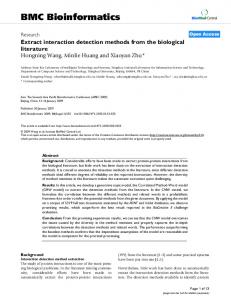
Results Algorithm The algorithm consists of several steps performed consecutively. First, given a wild-type sequence with several input parameters, the suboptimal solutions of the minimum free energy folding prediction are calculated. This step is followed by a suboptimal solutions filtering step. Next, the beginning and end points of each stem in the suboptimal solution results are calculated. Finally, mpoint mutations that disrupt the optimal solution are calculated. A summary of all the steps in the procedure is given in the flowchart available in Figure 1. Each step is described in detail below. Calculating suboptimal solutions After running the program, it calculates the dot-bracket representation of the optimal secondary structure of the given sequence, using the RNAfold routine of the Vienna RNA package, and the dot-bracket representations of all suboptimal secondary structures that are obtained using the RNAsubopt routine of the Vienna RNA package with some parameter -e (for calculating suboptimal structures within a range of kcals/mol of the mfe) are also calculated. This parameter is chosen by the user. The lower limit of e is 0. Regarding the upper limit, as will be elaborated in the Discussion Section, it is recommended to start for example from e = 15 for short sequences of about 70 nts with 3-point mutations and then to perform consecutive trials with increasing e until the optimal value is found for a particular case. In the case of sequences of about 70 nts and 3-point mutations, increasing e to high values such as 30 instead of 15 will yield a running time of days instead of seconds/minutes and is not desired. The program saves the optimal structure as "Opt" and all the suboptimal structures as a list called "Subopts". Filtering suboptimal solutions We use three filters on the "Subopts" list:

1) The first filter removes all suboptimal solutions for which the distance of their dot bracket representations from "Opt" is less than a parameter value ("dist1") as specified by the user ("dist1" is in the range from 0 to n). The distances are computed as described below. 2) The second filter is designed to simply discard the suboptimal solutions that most likely will not become the optimal solution after the introduction of an m-point mutation. For example, if the dot bracket representation




Figure 1 of the Proposed Procedure Flowchart Flowchart of the Proposed Procedure. A summary of each step in the suggested procedure.

of the optimal solution of the sequence UGCCUGCCUCUUGGGAGGGGC is .(((..((((....))))))) and the dot bracket representation of one of the suboptimals is ..((........))......., then it is clear that no one-point mutation can cause the optimal to become suboptimal. Compared to the other filters, the effect of such a filter is minor, and indeed it can be easily shut off as explained in connection with a threshold parameter called DIFF that will be described below. To generate such a filter, one could consider scenarios of hypothetical mutations in which a previously suboptimal solution becomes the optimal, but in such scenarios the location of the mutation is unknown, and therefore, we cannot measure the stability of such a structure using the Zuker-Turner energy rules [13]. However, we can apply a simplistic, highly approximate model that suits our requirements, one that will calculate the relative stabilities of the secondary structures of the optimal and all suboptimal solutions using a weighted Nussinov model [7] for assessing the strength of the base pairings. The base pairs CG and GC that are composed of three hydrogen bonds are given a score of 3, base pairs AU and UA that are composed of two hydrogen bonds are given a score of 2, and base pairs GU and UG that are traditionally considered a weaker bond compared to the former (e.g., early estimations described in [26]) are given a score of 1. After this calculation the filter removes those suboptimal

solutions with relative stabilities that are lower than that of the optimal as a consequence of the introduction of "numMuts" mutations (hypothetical mutations for which their exact location is unknown) into the wild-type sequence. For more information on how this filter operates and how to shut it off, see 'Additional file 1:Filter2' for supplementary information on the second filter. 3) The third filter removes the suboptimal solutions that are closest to each other, i.e., if the distance between two suboptimal solutions is less than a parameter "dist2" that is specified by the user ("dist2" is in the range from 0 to n), then one of the suboptimal solutions will be removed. As a pre-processing step, we prefer to remove solutions whose distances from the optimal are smallest and those deemed as less stable solutions. For this reason we sort all the remaining (after the two filters above) suboptimal solutions according to their distance from optimal in descending order and subsequently sort them according to their energy calculated by RNAsubopt. Only after the program is done with both sorting tasks is the third filter applied. We start from the first suboptimal solution (with the largest distance from optimal and the most stable), and check the distance of this solution against all other solutions. Each of the following solutions for which the distance from the first solution is less than "dist2" will be



removed from the list, but the first solution remains in the list. After reaching the end of the list, the second suboptimal solution becomes the first, and so on.


For example, one of the suboptimal solutions for the given sequence UGCCUGCCUCUUGGGAGGGGC is: ..(((.((....)).)))...

If the chosen parameters dist1 and dist2 (both ranging from 0 to n) are large numbers relative to the length of the sequence, then filtering is a fast process because most suboptimal solutions were filtered already with the first filter. Thus, the third filter, which has a quadratic running time of O(subs2) because we compare all pairs of suboptimal solutions, also appears to be fast. The running time of the first filter is O(subs), where "subs" is the number of suboptimal solutions obtained by running RNAsubopt on the wild-type RNA sequence. Calculating the distance between two dot-bracket representations In the future, we will offer a choice between three methods for calculating the distance between two dot-bracket representations of RNA secondary structures, but here we only used the two computationally faster techniques to present the methodology. The first method is Vienna's RNAdistance, which calculates a tree-edit distance by default. The second, more approximate method was developed to save time because we had too many suboptimal solutions to compare. Using this method we simply run the two dot-bracket representations in parallel and calculate the number of mismatches, or, equivalently, the Hamming distance. The running time is O(n), where n is the length of the dot-bracket representation. Finally, distances can also be calculated using the base pair distance that has been used in many previous studies (also available as an option in Vienna's RNAdistance). Similar to the Hamming distance, the base pair distance can be calculated efficiently with a running time of O(n). The current version of our application includes both the Hamming distance and the base pair distance as options for the user; the more expensive tree-edit distance could be added in the future. For example, suppose we have the following two dot brackets:

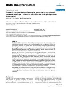
The dot plot (an n × n matrix with dots in the cells that correspond to base pairs) for this suboptimal solution has two stems (Figure 2). In all the dot plots presented in this work, it should be noted that we start the numbering from zero, and when referring to sequence positions in the dot plots this should be taken into account. The stems are represented by the starting and ending points, so the start of the first stem on this plot is location (2, 17) and the end of the first stem is location (4, 15). Similarly, the starting and the ending points of the second stem are (6, 13) and (7, 12) respectively. Calculating m-point mutations that disrupt the optimal solution We begin by searching for locations at which mutations in the dot plot may: (1) stabilize the suboptimal solution; (2) destabilize the optimal solution; and (3) simultaneously stabilize the suboptimal solution and destabilize the optimal solution. The stabilizing mutations in our case are mutations that extend the existing stems, or those that introduce an additional stem (with length > 1) near an existing stem, without disrupting any base pairs in the existing stems. The destabilizing mutations in our case are

((((.....)))) .((((....)))) The Hamming distance between the two dot-bracket representations is 2 (which is, in this case, the same value as the tree-edit distance calculated using RNAdistance with its default parameters), whereas the base pair distance is 8. Calculating the stems After we filter the suboptimal solutions, we calculate the stems for each suboptimal solution by calculating the starting and ending points of each stem in the suboptimal solution.

Figure 2 Solution in a Dot Plot Suboptimal Suboptimal Solution in a Dot Plot. Illustration of a suboptimal solution example in a dot plot. The solution is obtained by running Vienna's RNAsubopt for the sequence UGCCUGCCUCUUGGGAGGGGC.




mutations that disrupt some existing base pairs in the optimal solution without disrupting any base pairs in the suboptimal solution.

otides, which is unstable. On the other hand, it is possible that mutations in the hairpin are good if these mutations destabilize the optimal solution.

For example, location P(5, 14) for a mutation in the dot plot of Figure 2 signifies that a mutation in either nucleotide 5 or 14 on the RNA sequence forms a base pair between nucleotides 5 and 14. Note that P(5, 14) extends both stem1 and stem2, even connecting them, and as such it stabilizes the suboptimal solution shown in Figure 2. Additionally, P(1, 18) and the double location P(1, 18), P(0, 19) are also stabilizing locations because they extend stem1. All the "stabilizing" mutations that we found on the dot plot (Figure 2) are highlighted by circles in Figure 3. Therefore, if we are only searching for stabilizing single point mutations, then P(5,14) or P(1,18) are candidates but not P(0,19) as it forms a lonely base pair, which is not stable, and as such it should be discarded. In the case of stabilizing two-point mutations there are also two possibilities, P(5,14), P(1,18) and P(1,18), P(0,19), while a three-point mutation would incorporate P(5,14), P(1,18), P(0,19). There are no four or greater-than-four point mutations for this suboptimal solution if we are considering only stabilizing mutations. The locations P(8,11) and P(9,10) are not stabilizing locations because they will lower the hairpin loop to fewer than three nucle-

Using the same sequence (UGCCUGCCUCUUGGGAGGGGC), the optimal solution is .(((..((((....))))))), and the corresponding dot plot is shown in Figure 4. In this Figure the suboptimal solution that appears in Figures 2 &3 and an optimal solution for the RNA sequence are observable. Figure 5 shows the probability dot plot obtained by running the Vienna RNA package on the same sequence. Based on Figures 4 &5, we can conclude that mutation G14C in location P(5,14) stabilizes the suboptimal solution by forming a CG base pair between nucleotides 5 and 14. This same mutation, however, also destabilizes the optimal solution by breaking a GC base pair between nucleotides 9 and 14. Therefore, the mutation G14C is both stabilizing and destabilizing. On the other hand, mutation G5C at the same location P(5,14) is only a stabilizing mutation, because it also forms a base pair between nucleotides 5 and 14 in the suboptimal solution and connects "stem 1" and "stem 2", but it has no disruptive effect on the optimal solution. Each of these mutations is worth checking, but we may assume that mutation G14C will have a stronger effect on the conformational rearrangement of the optimal solution. And indeed, if we introduce mutation G14C and use the Vienna RNA package, we can confirm that this is a confor-

Figure 3 Mutations in the Dot Plot Stabilizing Stabilizing Mutations in the Dot Plot. The stabilizing mutations found by applying the proposed method on the dot plot in Figure 1. The stabilizing mutations are highlighted in circles.

Figure 4and Suboptimal Solutions in a Dot Plot Optimal Optimal and Suboptimal Solutions in a Dot Plot. Both optimal and suboptimal solutions in a dot plot, drawn for the case of Figure 1, running Vienna's RNAsubopt for the sequence UGCCUGCCUCUUGGGAGGGGC.




Mutations G18C and G19A at locations P(1,18) and P(0,19) (Figure 3) are also both stabilizing and destabilizing mutations, while mutations on the hairpin of the suboptimal solution, at locations P(8,11) and P(9,10), are only destabilizing mutations. For example, mutation U8G at P(8,11) disrupts a UA base pair between bases 8 and 15 in the optimal solution, but this mutation has no effect on base pairs in the suboptimal solution. Implementation First, we describe the optional modes of operation available to the user according to the problem at hand ("method") when implementing the proposed methodology. Second, in Testing we analyze the results of two artificial examples in detail, reporting running times, parameter usage, and possible limitations. Third, we show two practical implementation examples taken from the full P5abc subdomain of the Tetrahymena thermophila group I intron ribozyme and the 5BSL3.2 sequence of a subgenomic hepatitis C virus (HCV) replicon.

Figure 5and Suboptimal Solutions in a Probability Dot Plot Optimal Optimal and Suboptimal Solutions in a Probability Dot Plot. The full probability dot plot, drawn for the case of Figure 1, as a result of running Vienna's RNAsubopt for the sequence UGCCUGCCUCUUGGGAGGGGC. mational rearranging mutation (Figure 6). A rearranging mutation means a drastic change in one of the secondary structure motifs as inspected by eye, such as two new hairpins forming instead of one, etc.

After identifying the stabilizing and destabilizing locations, the program calculates m-point mutations using these detected locations. There are four options, depending on the desired running time vs. the number of mutations to be tried, for calculating mutations: 1) In the first option, we only take into account the stabilizing locations and we can only extend the existing stems without making any new stems. The number of mutations in this option is bounded by (2s)m * 2m, where s is the number of stems in the suboptimal solution and m is the number of point mutations. The expression (2s) is needed because mutations may be introduced at both ends of the stem, and 2m is included because in each detected location we may introduce two different mutations. The number of

Figure 6 Structure Drawings for the Wild-type and Mutant Secondary Secondary Structure Drawings for the Wild-type and Mutant. Secondary structure drawings for the wild-type and the mutant as a consequence of applying the rearranging point mutation found by our method, for the example in Figure 1 (the example is for the sequence UGCCUGCCUCUUGGGAGGGGC).




mutations will be much lower because in practice the stems are relatively close to each other and it is impossible to perform m mutations near each stem; and in some cases, it will be impossible to perform even a single mutation near the ends of most stems. Even for the worst cases, however, the running time is better than in the existing version of RNAmute when (3n)mmutations are tried, n being the length of the sequence and s