Apr 15, 2004 - In the de BroglieâBohm formulation of quantum mechanics the ... In this paper we formulate the Bohmian dynamics on subspaces and define ...
JOURNAL OF CHEMICAL PHYSICS
VOLUME 120, NUMBER 15
15 APRIL 2004
ARTICLES Bohmian dynamics on subspaces using linearized quantum force Vitaly A. Rassolov and Sophya Garashchuk Department of Chemistry & Biochemistry, University of South Carolina, Columbia, South Carolina 29208
共Received 16 December 2003; accepted 21 January 2004兲 In the de Broglie–Bohm formulation of quantum mechanics the time-dependent Schro¨dinger equation is solved in terms of quantum trajectories evolving under the influence of quantum and classical potentials. For a practical implementation that scales favorably with system size and is accurate for semiclassical systems, we use approximate quantum potentials. Recently, we have shown that optimization of the nonclassical component of the momentum operator in terms of fitting functions leads to the energy-conserving approximate quantum potential. In particular, linear fitting functions give the exact time evolution of a Gaussian wave packet in a locally quadratic potential and can describe the dominant quantum-mechanical effects in the semiclassical scattering problems of nuclear dynamics. In this paper we formulate the Bohmian dynamics on subspaces and define the energy-conserving approximate quantum potential in terms of optimized nonclassical momentum, extended to include the domain boundary functions. This generalization allows a better description of the non-Gaussian wave packets and general potentials in terms of simple fitting functions. The optimization is performed independently for each domain and each dimension. For linear fitting functions optimal parameters are expressed in terms of the first and second moments of the trajectory distribution. Examples are given for one-dimensional anharmonic systems and for the collinear hydrogen exchange reaction. © 2004 American Institute of Physics. 关DOI: 10.1063/1.1669385兴
by the wave function , the quantum potential is defined as
I. INTRODUCTION
Quantum-mechanical effects on the dynamics of nuclei are essential for a description of many chemical reactions. For large molecular systems, the exact methods of solving the Schro¨dinger equation are unfeasible, because of their exponential scaling with system size, while the methods of molecular dynamics, based on classical mechanics and applicable to high-dimensional systems, do not describe quantum effects. Therefore, great effort went into the development of semiclassical time-dependent methods that would combine favorable scaling of classical trajectory methods with a description of the dominant quantum effects in the limit of large mass or small ប appropriate for a description of molecules. We find that the de Broglie–Bohm formulation of the Schro¨dinger equation can serve as a very good starting point for the development of semiclassical time-propagation methods. Traditional semiclassical methods, such as the van Vleck–Gutzwiller propagator1 and initial-value representation methods,2– 4 are based on the stationary phase approximation to the Schro¨dinger equation. They involve the purely classical time evolution of trajectories with the quantum effects coming from summation over classical paths using the action and stability of classical trajectories. In contrast, in the de Broglie–Bohm formulation5 the Schro¨dinger equation can be solved in terms of quantum or Bohmian trajectories, evolving in time according to classical equations of motion, but under the influence of the quantum potential in addition to an external potential. For a particle of mass m described 0021-9606/2004/120(15)/6815/11/$22.00
U⫽⫺
ប 2 ⵜ 2兩 兩 . 2m 兩 兩
Bohmian trajectories can be a useful visualization tool6 and the formalism has been adapted to nonadiabatic dynamics,7,8 phase-space representations, and density matrix approaches.9–15 Numerical implementation of the quantum trajectory formulation is hindered by the special features of quantum trajectory dynamics: 共i兲 quantum trajectories cannot cross and 共ii兲 the quantum potential is, in general, singular when the density of the wave function vanishes. These properties lead to complicated and rapidly varying in time and space quantum potentials and quantum forces, which are very difficult to compute accurately. In recent years the quantum trajectory propagation method gained attention as an alternative way of solving the Schro¨dinger equation. Several approaches based on a local interpolation of the wave function density were suggested16 –20 and some of them proved to be efficient for model problems in many dimensions. Nevertheless, for general problems the accuracy of the quantum potential and consequently that of dynamics was found to deteriorate with time or to become impractical.21,22 This motivates us to focus on the Bohmian formulation as a basis for semiclassical propagation methods that use an approximate quantum potential 共AQP兲. As follows from the definition of the quantum potential, the classical limit in the Bohmian formulation can be defined as the quantum potential being zero in the limit of ប→0 or m→⬁. This implies a 6815
© 2004 American Institute of Physics
6816
J. Chem. Phys., Vol. 120, No. 15, 15 April 2004
certain behavior and properties of 兩兩, such as 兩兩⫽0. When the AQP is determined with high accuracy the formulation becomes equivalent to the full quantum mechanics. We are interested in the intermediate regime when the AQP is smooth enough for efficient and practical implementation in many dimensions, and at the same time, it is accurate enough to describe leading quantum effects in semiclassical systems.23 For example, fitting of the wave function density in terms of a single Gaussian function determines an AQP which is exact for a Gaussian wave packet evolving in a locally quadratic potential. This AQP also gives a good description of scattering on a barrier in one dimension.24 A recently proposed trajectory derivative propagation method of Trahan et al.25 effectively involves approximations for individual trajectories: the quantum potential is determined from auxiliary equations on the derivatives of the density and action function, and truncation of the infinite hierarchy of equations at a finite level 共such as second or third order兲 leads to ‘‘approximate Bohmian trajectories.’’26 Originally, we determined the AQP from the wave function density approximated in terms of fitting functions 共the number of the fitting functions controls the accuracy and numerical cost兲.23 We found that the resulting AQP did not conserve energy in a closed system, because the low-density regions are ‘‘underweighted’’ in the global density fit, whereas the quantum potential can be large in these regions. Then we found that the nonclassical component of the moជ 兩 兩 , might be a betmentum operator, proportional to 兩 兩 ⫺1 ⵜ ter candidate for the development of approximations. This quantity is inherently linked to the quantum potential: the optimized nonclassical momentum defines the energyconserving AQP regardless of the quality of the representaជ 兩 兩 共Ref. 27兲. We also showed that a simple tion of 兩 兩 ⫺1 ⵜ linear approximation to the nonclassical momentum results in a linear optimization problem, which makes this method cheap in many dimensions. The linearized nonclassical momentum generates a linear quantum force 共LQF兲, which describes the quantum dynamics of a correlated Gaussian wave packet in a locally quadratic potential exactly. The LQF description is somewhat reminiscent of the thawed Gaussian method28 and variational Gaussian wave packet dynamics,29 since the linear nonclassical momentum corresponds to the Gaussian wave function density. However, in the LQF method, there is no assumption about the actual wave function density. Therefore, the wave packet bifurcations are describable within this approach, as was shown by computing the wave packet transmission probabilities for onedimensional scattering and for the collinear hydrogen exchange reaction.30 To go beyond the LQF within the framework of approximating the nonclassical momentum, one may approach a full quantum-mechanical description by increasing the flexibility of the fitting functions. If the fitting function can be represented in terms of a complete basis set, the description will be formally exact, though optimization with complicated fitting functions will be a nonlinear problem which significantly increases computational costs. In this paper we present a different strategy of approximating the nonclassical momentum on subspaces or domains, which allows us to
V. A. Rassolov and S. Garashchuk
keep the fitting functions simple. The presence of spatial domains is included in the definition of the quantum potential, which makes this approach energy conserving. With the nonclassical momentum linearized on domains, the optimization problem remains linear, as in the LQF, and is independent for each domain and each dimension. The introduction of domains improves the description for anharmonic potentials and non-Gaussian wave packets, as shown by studies of the reflection on the Eckart barrier, the description of the ground state of the Morse oscillator, the computation of spectra for anharmonic and metastable wells, and studies of dynamics for the collinear H3 system. Sections II A and II B summarize the quantum trajectory method and the globally defined energy-conserving AQP, which are needed to define Bohmian dynamics and the energy-conserving AQP on spatial domains 共Sec. II C兲. Numerical examples and a discussion are presented in Sec. III. Section IV concludes. The energy conservation and solution for linear fitting functions are given as Appendixes A and B.
II. THEORY A. Quantum trajectory formalism
Consider a quantum-mechanical system in N-dimenˆ sional Cartesian space, governed by the Hamiltonian H † ⫺1 ˆ ˆ ⫽ P M P /2⫹V, where M is a diagonal matrix of masses, 兵 M nn 其 ⫽m (n) . 共Single superscript indexes are used to label dimensions; subscript indexes are used to label trajectories.兲 The time evolution of the density and the phase of a wave function (xជ ,t),
共 xជ ,t 兲 ⫽A 共 xជ ,t 兲 exp
冉
冊
S 共 xជ ,t 兲 , ប
A 共 xជ ,t 兲 ⫽ 冑 共 xជ ,t 兲 , 共1兲
which is a solution of the time-dependent Schro¨dinger equation in the Lagrangian frame of reference, are defined by dS 共 xជ ,t 兲 pជ T M ⫺1 pជ ⫽ ⫺V⫺U, dt 2
共2兲
d 共 xជ ,t 兲 ជ • vជ 共 xជ ,t 兲 . ⫽⫺ⵜ dt
共3兲
The amplitude A(xជ ) and phase S(xជ ) are real functions, and ជ S(xជ ,t) is the hydrodynamic, or ‘‘classical,’’ pជ ⫽M vជ ⫽ⵜ momentum.31 U is a nonlocal time-dependent quantum potential: U⫽⫺
ជ T M ⫺1 ⵜ ជ A 共 xជ ,t 兲 ប2 ⵜ . 2 A 共 xជ ,t 兲
共4兲
Expression 共2兲 is the Hamilton–Jacobi equation for the classical action of a trajectory in the presence of a classical potential V and a quantum potential U. Equation 共3兲 is a continuity equation for a normalizable wave function density. Atomic units ប⫽1 will be used below. In order to implement Eqs. 共2兲 and 共3兲, the initial wave function is represented in a set of trajectories with initial conditions 兵 xជ i (0),pជ i (0) 其 . The initial momenta are defined by ជ S(xជ ,0). A certain amount the initial phase of (xជ ,0), pជ i ⫽ⵜ i of density within a volume element, d⌰(xជ i ,t)⫽⌸ ␦ x (n) i (t)
J. Chem. Phys., Vol. 120, No. 15, 15 April 2004
Bohmian dynamics
⫻(i⫽1,...,N), or a certain weight can be associated with the ith trajectory. For a closed system the trajectory weight w i remains constant in the course of dynamics:24 w i ⫽ 共 xជ i ,t 兲 d⌰ 共 xជ i ,t 兲 ⫽ 共 xជ i ,0兲 d⌰ 共 xជ i ,0兲 .
共5兲
The initial density of (xជ ,0), (xជ ,0), defines the initial value of the quantum potential U, which affects the subsequent dynamics of the system. Conservation of the total energy in a closed system leads to the following property of the quantum potential: dE ⫽ dt
冕 ជ
U 共 x ,t 兲 共 xជ ,t 兲 d⌰ 共 xជ ,t 兲 ⫽0. t
共6兲
B. Global energy-conserving approximation of the nonclassical momentum
As follows from the definition 共4兲, the quantum potential depends on the curvature of the wave function amplitude. Local interpolation of (xជ ,t), evaluation of the derivatives of (xជ ,t), and subsequent determination of the quantum potential and quantum force become expensive and inherently inaccurate for the low-density regions. Therefore, we look for a global approximation to the ‘‘nonclassical momentum’’ ជ (xជ ,t) 共Ref. 27兲, proportional to the difrជ (xជ ,t)⫽ (xជ ,t) ⫺1 ⵜ ference between the quantum-mechanical momentum operator pˆ and the classically defined, or hydrodynamic, momenជ S 共Ref. 31兲. Each spatial component of rជ (xជ ,t), tum pជ ⫽ⵜ 共7兲
is approximated by a function of xជ of the general form g (n) (xជ ,sជ ) with K time-dependent parameters forming the vector sជ . For each dimension we define a functional
冕
关 r 共 n 兲 共 xជ ,t 兲 ⫺g 共 n 兲 共 xជ ,sជ 兲兴 2 共 xជ ,t 兲 d⌰ 共 xជ ,t 兲 ,
共8兲
which after trajectory discretization of the initial density (xជ ,0), I (n) can be rewritten as weighted sum over trajectories: I
共n兲
⫽I 共0n 兲 ⫹
兺i w i
冉
2
g 共 n 兲 共 xជ i ,sជ 兲 x
共n兲
冊
⫹g 共 n 兲 共 xជ i ,sជ 兲 2 .
ជ I 共 n 兲 ⫽0. ⵜ s
共10兲
˜ in terms of g (n) (xជ ,sជ ) is An approximate quantum potential U ˜ ⫽⫺ U
1
兺 n⫽1 8m 共 n 兲
冉
g 共 n 兲 共 xជ ,sជ 兲 2 ⫹2
g
共n兲
共 xជ ,sជ 兲
x
共n兲
冊
.
Let us divide the coordinate space into several subspaces or domains labeled l⫽1,...,L, each one defined by a ‘‘domain’’ function ⍀ l (x): ⍀ l (x)⭓0 for all x. For the sake of clarity the presentation below is given for a one-dimensional system; a generalization to many dimensions is outlined in Appendix A. These subspaces may correspond to physically significant regions such as reactants, products, and transition states in reactive dynamics, or they can be based on other considerations, such as the shape of the wave functions and features of the potential V. The domains are fixed in time and, in general, overlap in space. We choose the last domain with index L to complement the rest of the domains to unity, ⍀ L 共 x 兲 ⫽1⫺
共9兲
ជ I (n) 0 abbreviates a term that does not depend on s . The fact that neither (xជ ,t) nor its derivatives are involved is of central importance for an efficient implementation algorithm, which in this case will be linear with respect to the number of trajectories. The optimal values of sជ can be found from gradients of I (n) with respect to all components of sជ :
N
˜ evaluated at the optimal valAs we have shown earlier,30 U ues of sជ satisfies Eq. 共6兲 and, therefore, conserves the total energy of a closed system regardless of the functional form of g (n) . The simplest physically meaningful choice, corresponding to a Gaussian density, is to approximate r (n) with a linear function g (n) for each spatial component. This functional form for g (n) generates a quadratic approximate quantum ˜ and a LQF. The optimal values of the parameters potential U ជs , given by Eq. 共10兲, are found analytically from the first and second moments of the trajectory distribution 共see Appendix A兲, resulting in an efficient propagation scheme, which scales linearly with respect to the number of trajectories. From the theoretical point of view, the assumption of a linear nonclassical momentum is exact for a Gaussian wave packet evolving in time in a locally quadratic potential and it can describe dominant quantum effects in semiclassical systems. In order to improve the description of non-Gaussian wave functions and general potentials, we have to increase the flexibility of the fitting functions g (n) . A more sophisticated functional form 共up to g (n) being a linear combination of the functions forming a complete basis兲 could serve this purpose. Alternatively, the nonclassical momentum can be approximated with the fitting functions of restricted functional form on subspaces rather than on the full space, generalizing Eqs. 共8兲–共11兲.
C. Approximation on subspaces or spatial domains
1 共 xជ ,t 兲 r 共 n 兲 共 xជ ,t 兲 ⫽ , 共 xជ ,t 兲 x 共 n 兲
I 共 n 兲⫽
6817
共11兲
兺
l⫽1,L⫺1
⍀ l共 x 兲 ,
共12兲
so that the solution on the subspaces is equivalent to the solution on the full space. In order to solve the Schro¨dinger on a subspace, the kinetic energy operator Kˆ has to be modified to include the interface terms since ⍀ l (x) now enters the inner product. The Hermitian form of the kinetic energy matrix element, 具 i 兩 Kˆ 兩 j 典 , is 1 2m
冕 * i
⫽⫺
共 x 兲 j共 x 兲 ⍀ l 共 x 兲 dx x x
1 2m
冕
⍀ l共 x 兲 * i 共x兲
冋
2 x
2
⫹
册
⍀ l⬘ 共 x 兲 共 x 兲 dx. ⍀ l共 x 兲 x j 共13兲
6818
J. Chem. Phys., Vol. 120, No. 15, 15 April 2004
V. A. Rassolov and S. Garashchuk
With this form of Kˆ , for each domain the quantum potential U in Eq. 共2兲 is replaced by its modified version U l with the additional interface term U l ⫽⫺
冉
冊
1 A ⬙ 共 x,t 兲 ⍀ ⬘ 共 x 兲 A ⬘ 共 x,t 兲 ⫹ . 2m A 共 x,t 兲 ⍀ 共 x 兲 A 共 x,t 兲
共14兲
Equation 共3兲 for the density on a domain is also modified: ⍀ ⬘共 x 兲 d 共 x,t 兲 ⫽⫺ v ⬘ 共 x,t 兲 ⫺ v 共 x,t 兲 . dt ⍀共 x 兲
共15兲
Note that (x,t) and S(x,t) are still defined on the full space, not on the domains. The summation of Eq. 共15兲 over all domains weighted by ⍀ l gives Eq. 共3兲, since 兺 ⍀ l (x) ⫽1 and 兺 ⍀ ⬘l (x)⫽0 for domain functions satisfying Eq. 共12兲. This formulation is formally equivalent to the Schro¨dinger equation on the full space and offers no advantage if the quantum potential is determined exactly. But it enables us to define an approximate quantum potential on domains. We can approximate the nonclassical momentum on each domain by minimizing a functional I l⫽
冕 冉 ⬘
共 x,t 兲 ⫺g l 共 x,sជ 兲 共 x,t 兲
冊
2
⍀ l 共 x 兲 共 x,t 兲 dx,
共16兲
where sជ is a collection of the fitting parameters. The contribution to the approximate QP from each domain is determined by Eq. 共14兲: ˜ ⫽⫺ 1 兵 关 g 共 x,sជ 兲 2 ⫹2g ⬘ 共 x,sជ 兲兴 ⍀ 共 x 兲 U l l l l 8m ⫹2g l 共 x,sជ 兲 ⍀ ⬘l 共 x 兲 其 .
共17兲
The total quantum potential is a simple sum over domains: ˜⫽ U
兺
l⫽1,L
˜ . U l
共18兲
˜ should be evaluated at the optimal values of sជ that miniU ជ I ⫽0. Then, the approximate mize Eq. 共16兲 and for which ⵜ s l quantum potential defined on domains will rigorously conserve energy in a closed system, as was the case with the full space approximation, Eq. 共11兲. The derivation is given in Appendix A. We do not have to solve Eq. 共15兲 for the density, because once summed over the domains, it is equivalent to Eq. 共3兲. The latter can be solved for closed systems without approximations apart from the trajectory discretization, as given in Eq. 共5兲. In our approach we use spatial domains to approximate the nonclassical momentum and to define the AQP, while the wave function remains defined in the full space according to Eq. 共1兲. Within the quantum trajectory approach, it might be possible to describe the dynamics of unbound systems on a subspace, rather than on full space, according to Eqs. 共14兲 and 共15兲, since the effect of a given trajectory, moving in the asymptotic region toward infinite xជ on the rest of the trajectories, vanishes according to the domain function. This intriguing possibility, however, is beyond the scope of present paper.
As a practical implementation of the AQP defined on subspaces, we will use the linear fitting functions g l (x,sជ ) with different values of the parameters sជ for each domain. With this choice, the optimal parameters sជ are found by means of linear algebra in terms of first and second moments of the trajectory distribution independently for each domain. This solution is given in Appendix B. III. RESULTS AND DISCUSSION
In the preceding section we have described a rigorous way to define the quantum potential in terms of the approximate nonclassical momentum optimized on domains. This procedure gives an exact quantum potential if the fit of rជ (xជ ,t) were perfect. In practical applications to semiclassical systems we want to keep the number of domains small and to work with linear fitting functions. This leads to the issue of the domain setup. An efficient choice of a limited number of domains has to be based on some knowledge about the problem at hand: we set up domains in the regions of strong anharmonicity of the potential accessible to the quantum trajectories representing a given wave function. For the reactive scattering problem we set up separate domains to represent the reaction channels and transition state. The model systems studied below are chosen for their relevance to problems of nuclear dynamics. In all examples the quantum-mechanical results used for comparison were obtained using the splitoperator method.32 A. Scattering on the Eckart barrier
A standard one-dimensional test for semiclassical propagation methods is the scattering of a wave packet on a barrier. The computation of the transition probabilities within the frame work of quantum trajectories appears to be quite straightforward,17,23 while an accurate description of the reflected wave function presents a challenge. The reason for this is that the reflected component of the wave function interferes with the slow incoming component creating a ‘‘rippled’’ density profile. This caused instabilities in methods based on local density interpolation and derivative evaluation, which initiated the development of more sophisticated trajectory approaches such as moving grids33 or wave function transformation between representations.22 We study scattering on the Eckart barrier, V⫽D cosh(zx)⫺2, mimicking the transition state of the H3 system. The parameters of the potential are D⫽16, z⫽1.3624 in scaled atomic units, where the reduced mass of the hydrogen molecule is set to 1. The distance is measured in bohr, m⫽1. The initial wave packet is centered to the left of the barrier:
共 x,0兲 ⫽ 共 2 ␣ 0 / 兲 1/4 exp关 ⫺ ␣ 0 共 x⫺x 0 兲 2 ⫹ p 0 共 x⫺x 0 兲兴 . 共19兲 The choice of initial parameters as 兵␣ 0 ⫽6, x 0 ⫽2, p 0 ⫽3其 defines a wave packet with initial energy of about half the barrier height. Since we use Eq. 共5兲 for the amount of density within a volume element and do not compute the density explicitly, we examine quantities that can be computed directly as a sum over trajectories 共labeled by the index i兲, such as the reaction probability of a wave packet, P, defined as P⫽limt→⬁ 兺 i w i h„x i (t)… 关 h(x) is the Heaviside function兴.
J. Chem. Phys., Vol. 120, No. 15, 15 April 2004
Bohmian dynamics
FIG. 1. Scattering on the Eckart barrier. a兲 The domain set up: the potential 共scaled兲 is shown with a dashed line; the sum of five Gaussian domains described in text, is represented with a dot-dashed line; the complimentary domain is shown with a thin solid line; the wavefunction density; t at t⫽0.8, is shown with a thick solid line. b兲 The density overlap, 具 0 兩 t 典 obtained exactly 共QM兲 and using AQP defined on the full space 共LQF兲 and with six, L⫽6, and twenty, L⫽20, domains. Numbers in parentheses show the wavepacket transmission probability for these four calculations, respectively.
The quality of the description of the reflected component of a wave packet is assessed from a time-dependent overlap of the initial density 0 with the evolving density t : C 共 t 兲 ⫽ 具 0兩 t典 ⫽
兺i 兩 共 x i共 t 兲 ,0兲 兩 2 w i .
共20兲
The domains are chosen as Gaussian functions, ⍀ l 共 x 兲 ⫽exp关 ⫺  共 x⫺q l 兲 2 兴 ,
6819
are defined by setting q 1 ⫽⫺2.0, q l⫹1 ⫺q l ⫽0.5, and ⫽5.0. Trajectories were propagated up to t⫽1.5 with an increment of 0.0025. For the given wave packet the quantum value of the transmission probability is P QM⫽0.151. With U⫽0, the classical value of P is zero, since the classical energy of each trajectory is lower than the barrier height. The quantum potential gives a spread in energies to the quantum trajectories. The LQF is accurate while the quantum potential energy is converted into the classical kinetic energy. It gives a fairly accurate value for the transmission probability of P LQF ⫽0.141, even though the quantum force in this approximation goes to zero as the reflected and transmitted components of the wave function separate. A comparison of the density overlaps C(t), which depend on the accuracy of the reflected wave function, are presented on Fig. 1共b兲. Using the six domains described above gives a more accurate C(t) compared to the LQF result, as C(t) rises and falls off around t⫽1.1, but the discrepancy at the maximum remains. The transmission probability in this calculation is P⫽0.150. Using more localized domains covering a larger subspace—19 Gaussian domains defined by 兵q 1 ⫽⫺3.75, q l⫹1 ⫺q l ⫽0.25, ⫽18.0其 and a complimentary domain—gives an accurate description of density overlaps and P⫽ P QM. The number of trajectories required to converge C(t) within 0.02 were 249 and 849 for calculations with 6 and 20 domains, respectively. Formally, there should be no restrictions on domain functions in the limit of perfect fitting of ⫺1 ⵜ and infinitely closely spaced trajectories. However, we find it useful to impose certain requirements of the functional form of ⍀ l . These restrictions are mainly due to the density discretization in terms of trajectories and of the restricted form of fitting functions. Narrow, step-function-like domains have high derivatives at the domain boundary q 0 . This makes interface contributions to the integrals, such as those of Eqs. 共B5兲 and 共B6兲, inaccurate. Another point is that in the case of an ideal fitting, the contributions to the quantum potential from adja⬘ (q 0 ) and cent domains cancel at q 0 , since ⍀ ⬘l (q 0 )⫽⫺⍀ (l⫹1) g l (q 0 )⫽g (l⫹1) (q 0 ). This is not the case for linear fitting functions. Therefore, we choose domain functions ⍀ l in such a way that their derivatives in the interface regions are smaller than the change in the fitting parameters, which also gives better convergence of these parameters with respect to the number of trajectories.
B. Anharmonic oscillators
共21兲
placed before and inside the barrier region, where the density is compressed as the wave packet encounters the barrier and t has a non-Gaussian shape. The centers of Gaussian domains form an equidistant grid. Their width is such that adjacent ⍀ l have an overlap of about 0.55, which makes the sum of Gaussian domains a smooth function. The Gaussian domain functions are normalized so that their sum does not exceed 1. There is also a domain, given by Eq. 共12兲, that compliments this sum to unity on the full space. As an illustration, Fig. 1共a兲 shows a sum of five Gaussian domains and the complimentary domain, as well as the potential and bifurcating wave function density at t⫽0.8. Gaussian domains
A description of the long-time dynamics of general nonlinear bound systems in terms of quantum trajectories is numerically challenging, even with the wave function provided, because in the quantum trajectory formulation the interference is described by complicated density variations, as discussed and illustrated in Ref. 34. Therefore, it is important to rationalize the applicability of the AQP for anharmonic systems in the context of nuclear dynamics. At first, we apply the AQP approach to the Morse oscillator problem. The potential V describes a nonrotating H2 molecule, V⫽D 兵 1⫺exp关⫺z(x⫺xe)兴其2. With m⫽1.15, the parameters of the potential in scaled atomic units are D ⫽160.0, r e ⫽1.40 bohr, and z⫽1.0. We apply the quantum
6820
J. Chem. Phys., Vol. 120, No. 15, 15 April 2004
V. A. Rassolov and S. Garashchuk
FIG. 3. Dynamics in the potential with quartic anharmonicity. a兲 The amplitude of the auto-correlation function, C(t), as a function of time obtained with the LQF method 共solid line兲 and using two domains 共dashed line兲. The quantum result is shown with a dot-dashed line. b兲 The energy spectrum of C(t), I(E). The LQF, the two-domain and the exact results are shown with the solid line, dashed line and filled circles, respectively. The amplitude of the spectra for E⬎2.0 is multiplied by a factor of 10.
FIG. 2. Time-evolution of the Morse oscillator ground state. a兲 The average position as a function of time obtained quantum-mechanically 共thin solid line兲, using LQF on the full space 共dash兲, and using three 共dot-dash兲 and five 共thick solid line兲 domains. b兲 Real part of the auto-correlation function. The legend is the same as in panel a兲.
trajectory formalism to the propagation of the ground state (x,0) and examine the average position 具 x(t) 典 ⫽ 兺 i w i x i (t) and a more sensitive quantity: the autocorrelation function, which for a real initial wave packet is C 共 2t 兲 ⫽ 具 * 共 x,t 兲 兩 共 x,t 兲 典 ⫽
兺i w i exp关 2 S 共 x i ,t 兲兴 . 共22兲
Within the quantum trajectory formalism, the description of an eigenstate means that the quantum force exactly cancels the effect of the external potential and trajectories do not move, which is difficult to obtain with an approximate quantum force. From Fig. 2 we see that for the ground state the LQF works for short times: the anharmonicity of the potential leads to a large net force at the tails of the wave functions. For trajectories that start out on the steep side of the potential the net force is large and they move toward large values of x. Even though the weight of these trajectories is small, this behavior leads to incorrect values of the LQF parameters and ‘‘drains’’ energy from the remaining trajectories. Figure 2共a兲 shows the average position of the wave packet for a few oscillation periods: 具 x(t) 典 obtained with the LQF method shifts toward the dissociation region of V, whereas the exact value should stay as a constant. To de-
scribe the anharmonic regions of the potential better, we introduce two Gaussian domains, given by Eq. 共21兲, centered on the steep wall and at the bottom of the well: q 1 ⫽0.9, q 2 ⫽1.4, and  1,2⫽6.0. The complementary domain covers the dissociation region of the potential. As can be seen from Fig. 2, this reduces the amount of overenergetic trajectories—具 x(t) 典 grows much slower compared to the LQF calculation, and the accuracy of the correlation function is drastically improved. We still see the effect of the incorrect energy distribution: the oscillations of the phase of C(t) slow down as a function of time, as more trajectories move toward large x. The addition of another two Gaussian domains on the dissociation side reduces this effect and gives an accurate description of 具 x(t) 典 and C(t) for about two and a half oscillation periods. For this system the semiclassical C(t) is converged within 0.001 with 99 trajectories. The second example is the dynamics of a Gaussian wave packet in the anharmonic potential studied in Ref. 35. The potential is a harmonic oscillator perturbed by a quartic potential: V⫽x 2 /2⫹0.01x 4 ⫺1, m⫽1. The initial wave function is a displaced Gaussian, given by Eq. 共19兲, with the values ␣ 0 ⫽0.5, x 0 ⫽1.0, and p 0 ⫽0.0. We examine the autocorrelation function C(t) defined by Eq. 共22兲 and the spectrum of damped C(t):
冋冕
I 共 E 兲 ⫽Re
T
0
2
册
C 共 t 兲 e ⫺ ␥ t e Et dt .
共23兲
C(t) was obtained for nine oscillation periods (T⫽57.0) by propagating 399 trajectories with the time increment of 0.05, which gave a convergence of 兩 C(t) 兩 within 0.02. The damping is introduced to reduce the artifact of the finite propagation time. The value of the damping function at T is 0.01. The results of the LQF and of the two-domain calculations are shown in Fig. 3 in comparison to the exact quantum result. From the spectrum, we can see that the initial wave packet, which is displaced relative to the bottom of the well, has components from the five lowest eigenstates of the po-
J. Chem. Phys., Vol. 120, No. 15, 15 April 2004
tential. On this time scale the effect of anharmonicity is fairly small and linearization of the nonclassical momentum works well. We obtain all of the recurrences in C(t): the maxima are described accurately, while the amplitude of the minima shows deviations from the quantum result. The introduction of a single Gaussian domain 兵q 1 ⫽0.0,  1 ⫽2.5其 separating the bottom of the well from the high-energy regions of the potential largely removes this discrepancy in C(t). The agreement of the corresponding spectra is excellent, with the two-domain calculation having less ‘‘noise.’’ The energy spectrum for E⬎2.0 was multiplied by a factor of 10. The high accuracy of the semiclassical description is due to the slow accumulation of the effect of anharmonicity in this case. A two-peaked profile of the density develops after about ten oscillation periods. Effectively, we obtain C(t) from five oscillation periods during which the density becomes non-Gaussian, but it still has a single maximum. Thus the LQF works rather well. Interestingly, in the derivative propagation method calculation of Ref. 35 the effect of anharmonicity appears on a shorter time scale, resulting in the reproduction of two recurrences in C(t). In general, the description of the dynamics with the AQP for bound anharmonic systems, dominated by interference effects, will become impractical at long times. However, for high-dimensional systems, this type of behavior is, normally, quenched at short or intermediate times due to the decoherence of the wave function as, for example, was demonstrated in Refs. 36 –39. An approximate quantum potential approach might be accurate and efficient for these systems. C. Metastable potential well
As an example of a combined bound- and open-system dynamics we consider a metastable well studied in Ref. 14 with entangled trajectory molecular dynamics, combining the Bohmian formulation with the Wigner phase-space representation. The classical potential in scaled units with m⫽1 is V⫽Z(x 2 ⫺x 3 ), where Z⫽200. Here V forms a well, supporting two metastable states. The energy of the barrier top, located at x † ⫽0.667, is V † ⫽29.619. The potential of the unbound region is set to a constant: V⫽⫺V † for x ⬎1.1184. We examine the time evolution of two wave packets, defined by Eq. 共19兲 and initially centered on the repulsive wall, with total energies E tot⫽2V† and E tot⫽V†. The parameters of (x,0) are ␣ 0 ⫽10.0, p 0 ⫽0.0 with q 0 ⫽⫺0.4125 and q 0 ⫽⫺0.2821 for the two values of E tot . Figure 4 shows the amount of wave function density in the metastable well—the survival probability P(t) ⫽ 兺 x i (t)⬍x † w i and the energy spectrum of the autocorrelation function. Convergence for P(t) within 0.02 was achieved by propagating 499 and 999 trajectories with a time step of 0.0025 for the two values of the total energy, respectively. Classically (U⫽0), the energy of each trajectory remains constant in the course of dynamics and all trajectories with energies exceeding V † escape on a short time scale (t ⬇0.25). Quantum mechanically, the density continues to escape from the well, as the energy of quantum trajectories undergoes certain redistribution. Since the system shows strong quantum effects over an extended time, the linear ap-
Bohmian dynamics
6821
FIG. 4. Dynamics in the metastable well. a兲 Amount of the wavepacket in the well as a function of time. The upper three curves describe the classical 共dot-dash兲, the AQP with 10 domains 共dash兲 and the quantum 共solid line兲 results for the wavepacket with the total energy equal to the barrier height, E tot ⫽V † . The lower three curves show the same quantity 共the same legend, all lines are bold兲 for the wavepacket with the total energy of T tot ⫽2V † . b兲 The quantum and the AQP spectra are shown with solid line and squares, respectively, for the E tot ⫽V † system, and with dashed line and circles for the E tot ⫽2V † system.
proximation to the nonclassical momentum on the full space is inaccurate. We find that the introduction of nine domains reproduces the effect of density leaking out of the well. The domains are defined by Eq. 共21兲 with parameters q 1 ⫽⫺1.0, q l⫹1 ⫺q l ⫽0.25, and ⫽20.0. The Fourier transform of the autocorrelation function resolves the energy levels. The spectra shown in Fig. 4 were computed from the correlating functions obtained for t⫽ 关 0.0,2.0兴 and damped by exp(⫺␥t2) with ␥⫽2.3. To summarize, our one-dimensional studies show that generalization of the energy-conserving AQP method to multiple spatial domains increases the applicability of the linearized nonclassical momentum approach. Using a few spatial domains, we were able to reproduce accurately and efficiently a variety of quantum-mechanical effects on semiclassical wave packet dynamics, such as tunneling in open and quasibound systems, the zero-point energy effect, and resolution of the energy levels. The method is exact for Gaussian wave packets in a locally quadratic potential and can reproduce the effects of the distortion of the Gaussian density on the dynamics. Nevertheless, an efficient description of bound systems
6822
J. Chem. Phys., Vol. 120, No. 15, 15 April 2004
V. A. Rassolov and S. Garashchuk
with complicated dynamics, such as long-time dynamics in a double well, typical for proton transfer reactions or surface crossing problems, remains an outstanding challenge. An efficient description of the wave packet interference effect is essential for studies of these systems, whose behavior goes beyond the semiclassical regime. Interference is accompanied by the development of density nodes with small wave function amplitude, which makes the transition to the classical limit, U→0 as ប→0, impossible. Our example with the Eckart barrier shows that the development of an interference pattern can be described by performing linearization of the nonclassical momentum on small domains, but it becomes increasingly impractical for longer times. Except for the case of excited eigenstates, the quantum potential, quantum force, and nonclassical momentum have a 1/x-type singularity at the node, and linear functions, even ‘‘modulated’’ by the domain functions, are inefficient in this situation. Addressing the problem of a practical description of the wave function nodes is needed to extend the applicability of the AQP to the dynamics of bound systems dominated by interference effects. In its present form, our approach is capable of an efficient description of wave packet bifurcations, effects of distortion of the Gaussian density on dynamics, and redistribution of energy between quantum trajectories, which are the main features of semiclassical dynamics.
D. Dynamics in the collinear H3 system
The collinear hydrogen exchange reaction HA ⫹HB HC →HA HB ⫹HC is a standard test in reaction dynamics and presents a considerable challenge for semiclassical approaches. Recently, we have computed the wave packet transmission probabilities and studied the isotope effect for this system using the LQF.30 The system is described in the Jacobi coordinates of reactants where the kinetic energy is diagonal. The Hamiltonian, coordinates, and potential surface are the same as in Ref. 40. The initial wave packet is defined as
共 0 兲⫽
冑
2 共 ␣ ␣ 兲 1/2 exp关 ⫺ ␣ 1 共 R⫺R 0 兲 2 ⫺ ␣ 2 共 r⫺r 0 兲 2 1 2
⫹ p 0 共 R⫺R 0 兲兴 ,
共24兲
where r is the vibrational coordinate of the diatomic, the distance between HB and HC , and R is the translational degree of freedom—the distance between HA and the diatomic. In the Jacobi coordinates of reactants the angle , ⫽arctan(r/R), is used to divide the potential energy surface into the reactant region 0⬍⭐/6 and product region /6 ⬍⬍/3. The surface is symmetric with respect to 0 ⫽ /6. Values of the parameters in atomic units 共scaled by the reduced mass of the diatomic, m H /2⫽1) are R 0 ⫽4.5, r 0 ⫽1.3, ␣ 1 ⫽4.0, ␣ 2 ⫽9.73, and p 0 ⫽ 关 ⫺15,⫺1 兴 . The scaled unit of time is equal to 918 a.u. The initial positions for the quantum trajectories xជ (0)⫽ 兵 R i ,r i 其 are chosen on a rectangular grid with spacings dR⫽0.017 and dr⫽0.020. Trajectory with weights smaller than 10⫺8 are not included. The initial momenta are pជ (0)⫽ 兵 p 0 ,0其 ; the initial classical actions are S i (0)⫽p 0 (R i ⫺R 0 ). We analyze the wave packet
transmission probability P(t), P(t)⫽ 兺 prod w i , where the i summation goes over the trajectories in the product region for which arctan 关 r i (t)/R i (t) 兴 ⬎ /6. For optimization using domains, the reactant and product channel are divided into two subspaces: the switching functions between the reactant and product channels are 1 2
arctan关 z 共 ⫺ /6兲兴 , 2 arctan共 z /6兲
1 2
arctan关 z 共 ⫺ /6兲兴 . 2 arctan共 z /6兲
reac⫽ ⫺
prod⫽ ⫹
共25兲
The slope parameter is z⫽10. In each channel three subspaces are introduced in the same way as for the onedimensional Morse oscillator in this section. In the reactant channels there are two Gaussian domains in the vibrational coordinate r, given by Eq. 共21兲, centered at q 1 ⫽0.9 and q 2 ⫽1.4, with the width parameter ⫽6.0, and a complimentary domain. The reactant domains functions are multiplied by reac . The product domains are symmetrical to the reactant domains with respect to ⫽/6 and are multiplied by prod . In addition, three two-dimensional Gaussian domains are specified in the transition state with appropriate modification of the reactant and product domains satisfying Eq. 共12兲, bringing the total number of domains to L⫽9. The transition-state domain functions are centered in the transition state around the minimum along ⫽/6 at q 7 ⫽2.1, q 8 ⫽2.6, and q 9 ⫽3.1 bohrs. The width parameter along the transition state was ⫽5.0 in both coordinates. The wave packets were propagated up to t⫽1.8 with step size of 0.0025. Using 2453 trajectories per wave packet gave values of P within 0.015 of the converged result. The wave packet reaction probability as a function of energy is presented on Fig. 5共a兲, which also shows the classical U⫽0 and LQF results. Optimization on full space gives a qualitative agreement with the quantum result. Optimization on the domains leads to improved probabilities, which are now within 0.04 of the quantum-mechanical values. For this system the main deficiency of the LQF method was the same as in the Morse oscillator example: an appreciable amount of the total energy was carried away by the trajectories from the repulsive wall. This was corrected by treating high regions of the potential surface within separate domains, which ‘‘uncouples’’ them from the low-energy regions, where most of the trajectories evolve. For a more detailed analysis of the method we examine the dynamics of the wave packet for which wave packet transmission probability is large and the quantum trajectory result is close to the quantum-mechanical calculation, p 0 ⫽⫺7.5. The time-dependent transmission probability is plotted on Fig. 5共b兲. Semiclassical P(t) has a smaller value at the maximum, showing that fewer trajectories entered the transition-state region compared to the exact dynamics. To examine the dynamics in the product channel, we have also computed the density overlap of the time-evolving density with the fixed wave packet on the product side, symmetrical to 共0兲, C(t)⫽ 具 (t) 兩 prod(0) 典 . The domain calculation agrees with the exact result qualitatively. The integral amount of transmitted density overlapping with prod,
J. Chem. Phys., Vol. 120, No. 15, 15 April 2004
FIG. 5. Dynamics of the collinear H 3 system. a兲 The wavepacket transmission probability as a function of the total energy of the wavepacket: quantum 共thick solid line兲, classical 共thin solid line兲, LQF 共thin dash兲 and the domain 共thick dash兲 results are shown. b兲 The wavepacket transmission probability as a function of time computed for the wavepacket with 0 ⫽7.5. The quantum and the domain results are shown with thick solid and dashed lines, respectively. Thin solid and dashed lines mark the corresponding reactant/ product density overlaps. c兲 The absolute value of the auto-correlation function for the transition state wavepacket as a function of time. The quantum and the domain results are shown with the solid and dashed lines, respectively. The insert shows the corresponding spectra 共the semiclassical spectrum with triangles兲.
兰 C(t)dt, agrees very well with the exact result. The buildup of the semiclassical C(t) is delayed, which might be the reason for the double-peaked profile, while the exact result has a smooth peak around t⫽1.0. The domain calculation reproduces rather well the short-time dynamics, which largely determines the total wave packet reactivity. The details of the long-time dynamics, affected by the presence of resonances in the transition state and implying interference effects in the wave function, are not captured. This feature is also manifested in the analysis of the transition-state wave packet. We propagate a Gaussian wave packet, given by Eq. 共24兲 located at t⫽0 in the transition state and displaced from its minimum. The initial parameters are 兵R 0 ⫽2.5, r 0 ⫽1.3, ␣ 1 ⫽6.3, ␣ 2 ⫽6.3, p 0 ⫽0.0其. Figure 5共c兲 shows its autocorrelation function for t⫽ 关 0.0,2.0兴 and the corresponding energy spectrum. Five two-dimensional Gaussian domains in the transition, whose centers form a grid along the ⫽/6 direction, q l ⫽ 兵 2.1,2.6,3.1,3.6,4.1其 bohrs, were used in this calculation. The width parameter in the direction of the transition state was ⫽8.0. The width parameter for the domain functions in the perpendicular direction was chosen to be smaller, ⫽2.0, to make these functions more delocalized, since the channel regions were described within a single domain each, defined by reac and prod . In this calculation we used 4281 trajectories, whose weights were greater than 10⫺6 , which gave a spectrum with amplitudes within 7% of the converged
Bohmian dynamics
6823
values. The position of the spectrum peaks is converged within its resolution. The number of trajectories is slightly greater in comparison to the probability calculations, because the autocorrelation function C(t) is a complex quantity. Our semiclassical method reproduced one recurrence in C(t) around t⫽1.0 and does not reproduce low-amplitude recurrences at later times. The inset in the figure shows the exact and the semiclassical spectra of C(t), which agree quite well. In general, the agreement of the semiclassical description with the full quantum-mechanical result depends on the level of detail one obtains. This is the case for scattering on the Eckart barrier discussed in the beginning of this section: the LQF gives an accurate description of the wave packet transmission, while details of the reflected wave function density are reproduced only with the introduction of a fairly large number of spatial domains. For the collinear H3 system we do not reproduce quantitatively the details of the reactant wave packet passing through the product channel, but we describe shorter-time dynamics accurately and obtain very good agreement for the wave packet transmission probabilities and for the medium-resolution transition-state spectrum, using the AQP optimized on domains. IV. CONCLUSIONS
In this paper we formulated the Bohmian dynamics on subspaces and defined the energy-conserving approximate quantum potential in terms of the optimized nonclassical moជ . The new strategy enables us to solve the mentum ⫺1 ⵜ optimization problem on the subspaces or spatial domains instead of the full coordinate space. Consequently, we can obtain a more accurate fitting of the nonclassical momentum using simple fitting functions in the optimization. In particular, optimization with linear fitting functions on domains is solved separately for each domain and for each dimension by means of linear algebra. This is a generalization of the linearized quantum force approximation we developed earlier. The optimization is performed for all trajectories at once at every time step, resulting in an efficient procedure that scales well with the number of dimensions. The scaling with respect to the number of trajectories is linear. The cost of propagating quantum trajectories with this type of AQP is essentially the same as in classical mechanics. An additional effort is to compute the first and second moments of the trajectory distribution in each domain, which is a linear operation with respect to the number of trajectories, and to invert the matrix of the size of the number of dimensions. The proposed AQP rigorously conserves energy in a closed system and describes the dynamics of a Gaussian wave packet in a locally quadratic potential exactly. The classical and quantum limits are well defined. Increased flexibility of the fitting functions results in more accurate AQP, which expands the applicability of our approach. In this paper we used the energy-conserving AQP to describe reflection from the barrier and dynamics in the anharmonic bound and quasibound one-dimensional systems. The new method is a significant improvement over the linearized quantum force approximation and is capable of
6824
J. Chem. Phys., Vol. 120, No. 15, 15 April 2004
V. A. Rassolov and S. Garashchuk
describing the main features of semiclassical dynamics, such as tunneling, wave packet bifurcation, zero-point energy, and quantum potential energy redistribution effects. The description of dynamics, dominated by the interference effects, such as the long-time dynamics of anharmonic bound systems, remains an outstanding challenge. This type of behavior is beyond the semiclassical regime in a sense that the system does not have a classical limit of vanishing quantum potential as ប→0, due to the nodes in the density. Since bound anharmonic potentials are encountered in nuclear dynamics, this problem must be addressed. We believe that in order to describe interference effects in a practical way, one has to account for singularities in the density by explicitly including the appropriate term, such as c(x⫺x 0 ) ⫺1 or its ‘‘smoothed’’ representation 2c(x⫺x 0 )/ 关 c(x⫺x 0 ) 2 ⫹1 兴 , into the definition of the fitting function g. These functional forms can be easily generalized to the multidimensional case. Optimization with respect to x 0 and c will be a more complicated 共compared to the present method兲 nonlinear problem, but optimization of the coefficient c as well as that for the linear part of g will remain linear, so that an efficient overall implementation might be developed. Studies of this issue are under way in our group. Application of the energyconserving AQP to the hydrogen exchange reaction shows that in its present form, the method can correctly describe short- and medium-time dynamics, which is demonstrated by very good agreement for the wave packet transmission probabilities and of a medium resolution spectrum for the transition-state wave packet dynamics. The long-time dynamics, dominated by the interference effects, is reproduced only qualitatively. Nevertheless, this method might be well suited for studies of complex molecular systems in high dimensions, where long-time quantum effects are effectively quenched.
APPENDIX A: ENERGY-CONSERVING APPROXIMATE QUANTUM POTENTIAL IN MANY DIMENSIONS
Equations 共16兲 and 共17兲 are generalized in a straightforward manner for N dimensions. For each domain defined by ⍀ l (xជ ) the functional I l includes summation over the dimensions n⫽1,...,N, I l⫽
兺n m 共 n 兲 冕 1
冉
1 共 xជ ,t 兲 ⫺g 共en 兲 共 xជ ,sជ 共l n 兲 兲 共 xជ ,t 兲 x 共 n 兲
冊
⫹
1
dg 共l n 兲 dx
共n兲
冉
冉
共A1兲
g 共l n 兲 共 xជ ,sជ 共l n 兲 兲 2 2
⍀ l 共 xជ 兲
冉
xជ ,sជ 共en 兲 ⍀ l 共 xជ 兲 ⫹g 共l n 兲 xជ ,sជ 共en 兲
d⍀ l 共 xជ 兲 dx
共n兲
共A3兲
l
Integrating Eq. 共A1兲 by parts one arrives at I l ⫽I 0 ⫹
⫹
兺n m 共 n 兲 冕 1
dg 共l n 兲 dx
共n兲
冉
g 共l n 兲 共 xជ ,sជ 共l n 兲 兲 2 2
⍀ l 共 xជ 兲
xជ ,sជ 共en 兲 ⍀ l 共 xជ 兲 ⫹g 共l n 兲
冉
⫻ xជ ,sជ 共en 兲
d⍀ l 共 xជ 兲 dx 共 n 兲
冊
共 xជ ,t 兲 d⌰ 共 xជ ,t 兲 ,
共A4兲
where I 0 does not depend on the fitting parameters and the remaining term is proportional to the domain contribution ˜ 典 . We use this, along with Eq. 共6兲, into the average AQP, 具 U ˜ to prove the energy conservation property. Substitution of U given by Eq. 共A2兲 instead of U into Eq. 共6兲 gives
冕
˜ dsជ 共l n 兲 U ជ 共 n 兲具 U ˜ 典 ⫽0. 共 xជ ,t 兲 d⌰ 共 xជ ,t 兲 ⫽ ⵜ t dt s l l,n
兺
共A5兲
APPENDIX B: OPTIMAL PARAMETERS OF THE LINEARIZED MOMENTUM ON SPATIAL DOMAINS IN MANY DIMENSIONS
In the case of linear fitting functions Eq. 共A4兲 can be written as a matrix equation for each spatial domain. The domain label l is omitted below. With index n labeling dimensions, a general linear function g (n) (xជ ,sជ (n) ) is represented as a scalar product of two vectors of length (N⫹1)—a vector of space variables, rជ ⫽ 共 x 1 ,x 2 ,...,x N ,1兲 T ,
共B1兲
and a vector of parameters, sជ 共 n 兲 ⫽ 共 s 1n ,s 2n ,...,s Nn ,s 0n 兲 T .
ជ (n)
ជ (n)
共B2兲
Then g (xជ ,s )⫽rជ •s . Organizing vectors s rectangular matrix S of size N⫻(N⫹1), (n)
ជ (n)
into a 共B3兲
Eq. 共A3兲 can be rewritten as a linear matrix equation
The total approximate quantum potential includes a double sum over the dimensions n⫽1,...,N and over the domains l ⫽1,...,L:
兺 l,n 8m 共 n 兲
ជ 共 n 兲 I ⫽0. ⵜ s l
S⫽ 共 sជ 共 1 兲 ,sជ 共 2 兲 ,...,sជ 共 N 兲 兲 ,
2
⫻ 共 xជ ,t 兲 d⌰ 共 xជ ,t 兲 .
˜ ⫽⫺ U
introduction of a multiplicative nonzero constant in front of each term of the sum in this expression does not change the optimal values of sជ (n) l , which satisfy
冊
M2 S⫽⫺M0 ⫺M1 ,
and then solved for S. The dimension of the matrix M2 , M2 ⫽ 具 rជ rជ T ⍀ 典 , is (N⫹1)⫻(N⫹1). Its elements are the first and second moments of the trajectory distribution weighted by the domain function: M i2j ⫽
. 共A2兲
The key point is that minimization of Eq. 共A1兲 can be done independently for each dimension and for each domain. The
共B4兲
冕
r 共 i 兲 r 共 j 兲 ⍀ 共 xជ 兲 d 共 xជ ,t 兲 d⌰ 共 xជ ,t 兲 .
共B5兲
The dimension of the matrix M0 is N⫻(N⫹1). Its diagonal elements are M ii0 ⫽
冕
⍀ 共 xជ 兲 共 xជ ,t 兲 d⌰ 共 xជ ,t 兲 .
共B6兲
J. Chem. Phys., Vol. 120, No. 15, 15 April 2004
Bohmian dynamics
Off-diagonal elements are zero. The matrix M1 containing the ‘‘interface’’ terms is of the same size as M0 , M1 ជ ⍀) T 典 . Its elements are ⫽ 具 rជ (ⵜ M i1j ⫽
冕
r共i兲
d⍀ 共 xជ 兲 dx 共 j 兲
共 xជ ,t 兲 d⌰ 共 xជ ,t 兲 .
共B7兲
In a numerical implementation the integrals in Eqs. 共B5兲– 共B7兲 are replaced by a summation over trajectories with (xជ ,t)d⌰(xជ ,t) represented by the trajectory weight w i according to Eq. 共5兲. M. Gutzwiller, Chaos in Classical and Quantum Mechanics 共SpringerVerlag, New York, 1990兲. 2 M. Herman and E. Kluk, Chem. Phys. 91, 27 共1984兲. 3 K. G. Kay, J. Chem. Phys. 100, 4377 共1994兲. 4 W. H. Miller, J. Phys. Chem. A 105, 2942 共2001兲. 5 D. Bohm, Phys. Rev. 85, 167 共1952兲. 6 A. S. Sanz, F. Borondo, and S. Miret-Artes, J. Phys.: Condens. Matter 14, 6109 共2002兲. 7 R. E. Wyatt, C. L. Lopreore, and G. Parlant, J. Chem. Phys. 114, 5113 共2001兲. 8 E. Gindensperger, C. Meier, and J. A. Beswick, J. Chem. Phys. 113, 9369 共2000兲. 9 I. Burghardt and L. S. Cederbaum, J. Chem. Phys. 115, 10303 共2001兲. 10 I. Burghardt and L. S. Cederbaum, J. Chem. Phys. 115, 10312 共2001兲. 11 I. Burghardt and K. B. Moller, J. Chem. Phys. 117, 7409 共2002兲. 12 J. B. Maddox and E. R. Bittner, J. Phys. Chem. B 106, 7981 共2002兲. 13 E. R. Bittner, J. B. Maddox, and I. Burghardt, Int. J. Quantum Chem. 89, 313 共2002兲. 14 A. Donoso and C. C. Martens, Phys. Rev. Lett. 87, 223203 共2002兲. 1
6825
C. J. Trahan and R. E. Wyatt, J. Chem. Phys. 119, 7017 共2003兲. B. K. Dey, A. Askar, and H. Rabitz, J. Chem. Phys. 109, 8870 共1998兲. 17 C. L. Lopreore and R. E. Wyatt, Phys. Rev. Lett. 82, 5190 共1999兲. 18 D. Nerukh and J. H. Frederick, Chem. Phys. Lett. 332, 145 共2000兲. 19 E. R. Bittner and R. E. Wyatt, J. Chem. Phys. 113, 8888 共2000兲. 20 R. E. Wyatt and K. Na, Phys. Rev. E 65, 016702 共2002兲. 21 E. R. Bittner, J. Chem. Phys. 113, 9703 共2000兲. 22 R. E. Wyatt and E. R. Bittner, J. Chem. Phys. 113, 8898 共2000兲. 23 S. Garashchuk and V. A. Rassolov, Chem. Phys. Lett. 364, 562 共2002兲. 24 S. Garashchuk and V. A. Rassolov, J. Chem. Phys. 118, 2482 共2003兲. 25 C. J. Trahan, K. Hughes, and R. E. Wyatt, J. Chem. Phys. 118, 9911 共2003兲. 26 J. B. Maddox and E. R. Bittner, J. Chem. Phys. 119, 6465 共2003兲. 27 S. Garashchuk and V. A. Rassolov, Chem. Phys. Lett. 376, 358 共2003兲. 28 E. Heller, J. Chem. Phys. 62, 1544 共1975兲. 29 R. D. Coalson and M. Karplus, J. Chem. Phys. 93, 3919 共1990兲. 30 S. Garashchuk and V. A. Rassolov, J. Chem. Phys. 120, 1181 共2004兲. 31 ជ S as the ‘‘classical’’ component of the moWe refer to the quantity p⫽ⵜ mentum operator by analogy with the momentum variable of classical mechanics. This quantity is equivalent to the momentum of classical mechanics at the classical limit of quantum potential being zero. 32 M. D. Feit, J. A. Fleck, and A. Steiger, J. Comput. Phys. 47, 412 共1982兲. 33 C. J. Trahan and R. E. Wyatt, J. Chem. Phys. 118, 4784 共2003兲. 34 Y. Zhao and N. Makri, J. Chem. Phys. 119, 60 共2003兲. 35 E. R. Bittner, J. Chem. Phys. 119, 1358 共2003兲. 36 R. Gelabert, X. Gimenez, M. Thoss, H. B. Wang, and W. H. Miller, J. Chem. Phys. 114, 2572 共2001兲. 37 H. B. Wang, M. Thoss, K. L. Sorge, R. Gelabert, X. Gimenez, and W. H. Miller, J. Chem. Phys. 114, 2562 共2001兲. 38 W. H. Miller, J. Phys. Chem. A 105, 2942 共2001兲. 39 M. Thoss, H. B. Wang, and W. H. Miller, J. Chem. Phys. 114, 9220 共2001兲. 40 S. Garashchuk and D. J. Tannor, Chem. Phys. Lett. 262, 477 共1996兲. 15 16