BOOK: Models of science dynamics - encounters between ... - arXiv

arXiv:1201.0676v1 [physics.soc-ph] 3 Jan 2012

BOOK: Models of science dynamics encounters between complexity theory and information sciences

CHAPTER 3

Knowledge epidemics and population dynamics models for describing idea diffusion Nikolay K. Vitanov and Marcel R. Ausloos

I

Abstract The diffusion of ideas is often closely connected to the creation and diffusion of knowledge and to the technological evolution of society. Because of this, knowledge creation, exchange and its subsequent transformation into innovations for improved welfare and economic growth is briefly described from a historical point of view. Next, three approaches are discussed for modeling the diffusion of ideas in the areas of science and technology, through (i) deterministic, (ii) stochastic, and (iii) statistical approaches. These are illustrated through their corresponding population dynamics and epidemic models relative to the spreading of ideas, knowledge and innovations. The deterministic dynamical models are considered to be appropriate for analyzing the evolution of large and small societal, scientific and technological systems when the influence of fluctuations is insignificant. Stochastic models are appropriate when the system of interest is small but when the fluctuations become significant for its evolution. Finally statistical approaches and models based on the laws and distributions of Lotka, Bradford, Yule, Zipf-Mandelbrot, and others, provide much useful information for the analysis of the evolution of systems in which development is closely connected to the process of idea diffusion.

1

10 important questions raised in this chapter 1. What is the connection between knowledge and capital? 2. What happens in the case of knowledge diffusion? 3. Should quantitative research be supplemented by qualitative research? 4. Who are the pioneers of scientometrics? 5. What is the relation between epidemic models and of population dynamics models? 6. What has to be done if fluctuations strongly influence the system evolution? 7. Why are discrete models useful? 8. Around which statistical law are grouped all statistical tools described in the chapter? 9. Are all possibly relevant models, presented in this chapter? 10. What is the strategy followed by the authors of the chapter?

and their answers in the form of guidance Knowledge is often considered as a form of human capital Knowledge is transferred when the subjects interact Yes, surely supplemented coordinated joint aims are useful Alfred Lotka and Derek Price Epidemic models are a particular case of population dynamics models Switch from deterministic to stochastic models and think Often data is collected for some period of time. Thus, such data is best described by discrete models Around Lotka law NO ! Only an appropriate selection. For more models, consult the literature or ask a specialist Proceed from simple to more complicated models and from deterministic to stochastic models supplemented by statistical tools

Table 1: Several questions and answers that should guide and supply useful and important information for the reader.

1 1.1

Knowledge, capital, science research, and ideas diffusion Knowledge and capital

Knowledge can be defined as a dynamic framework connected to cognitive structures from which information can be sorted, processed and understood [1]. Along economics lines of thought [2, 3, 4], knowledge can be treated as one of the ”production factors”, - i.e., one of the main causes of wealth in modern capitalistic societies. 2

Models described in this chapter

Science landscapes Verhulst Logistic curve Broadcasting model of technology diffusion Word-of-mouth model

Mixed information source model Lotka-Volterra model of innovation diffusion with time lag Price model of knowledge growth with time lag SIR models of scientific epidemics SEIR models of scientific epidemics

are useful for Evaluation of research strategies. Decisions about personal development and promotion Description of a large class of growth processes Understanding the influence of mass media on technology diffusion Understanding the influence of interpersonal contacts on technology diffusion Understanding the influence of both mass media and interpersonal contacts on technology diffusion Understanding the influence of the time lag between hearing about innovation and its adoption Modeling the growth of discoveries, inventions, and scientific laws Modeling the epidemic stage of scientific idea spreading Extends the SIR model by specifically adding the role of a class of scientists exposed to some scientific idea

Table 2: List of models described in the chapter with comments on their usefulness. According to Marshall [5] a ”capital” is a collection of goods external to the economic agent that can be sold for money and from which an income can be derived. Often, knowledge is parametrized as such a ”human capital” [6, 7, 8, 9, 10]. Walsh [11] was one pioneer in treating human knowledge as if it was a ”capital”, in the economic sense; he made an attempt to find measures for this form of ”capital”. Bourdieu [12], Coleman [13], Putnam [14], Becker and collaborators have further implanted the concept of such a ”human capital” in economic theory [15, 16, 17]. However, the concept of knowledge as a form of capital is an oversimplification. This global-like concept does not account for many properties of knowledge strictly connected to the individual, such as the possibility for different learning paths or different views, multiple levels of interpretation,

3

Models described in this chapter

are useful for

Discrete model for the change in the number of authors in a scientific field Daley model

Modeling and forecasting the evolution in the number of authors and papers in a scientific field Modeling the evolution of a population of papers in a scientific field Modeling and forecasting the joint evolution of population of scientists and papers in a research field Epidemic model for the increase of number of scientists from a research field who start work in a sub-field of the scientific field. The model also describes the increase in the number of papers in the research sub-field Understanding the joint evolution of scientific fields in presence of migration of scientists from one field to another field

Coupled discrete model for populations of scientists and papers Goffman-Newill model for the joint evolution of one scientific field and one of its sub-fields

Bruckner-Ebeling-Scharnhorst model for the evolution of n scientific fields

Table 3: List of models described in the chapter with comments on their usefulness (Continuing Table 2). and different preferences [18]. In fact, knowledge develops in a quite complex social context, within possibly different frameworks or time scales, and involves ”tacit dimensions” (beside the basic space and time dimensions) requiring coding and decoding [4].

FOR POLICY-MAKERS Take away box Nr.1: Knowledge is much more than a form of capital:it is a dynamic framework connected to cognitive structures from which information can be sorted, processed and understood.

1.2

Growth and exchange of knowledge

Science policy-makers and scholars have for many decades wished to develop quantitative methods for describing and predicting the initiation and growth of science research [19, 20, 21]. Thus, scientometrics has become one of 4

Models described in this chapter

are useful for

SI model for the probability of intellectual infection

Modeling the spread of intellectual infection along a scientific network Modeling the spread of intellectual infection along a scientific network in the presence of a class of scientists exposed to the intellectual infection Modeling the number of scientists in a research subfield as a stochastic variable described by a master equation Modeling the influence of fluctuations in scientific productivity through differential equations for the dynamics of a scientific community Understanding the competition between ideologies with possible migration of believers Modeling the change of research field as a migration process

SEI model for the probability of intellectual infection

Stochastic evolution model

Stochastic model of scientific productivity Model of competition between ideologies Reproduction-transport model

Table 4: List of models described in the chapter with comments on their usefulness (Continuation of Table 2). the core research activities in view of constructing science and technology indicators [22]. The accumulation of the knowledge in a country’s population arises either from acquiring knowledge from abroad or from internal engines [23, 24, 25, 26]. The main engines for the production of new knowledge in a country are usually: the public research institutes, the universities and training institutes, the firms, and the individuals [27]. The users of the knowledge are firms, governments, public institutions (such as the national education, health, or security institutions), social organizations, and any concerned individual. The knowledge is transferred from producers to the users by dissemination that is realized by some flow or diffusion of process [28], sometimes involving physical migration. Knowledge typically appears at first as purely tacit: a person ”has” an idea [29, 30]. This tacit knowledge must be codified for further use; after codification, knowledge can be stored in different ways, as in textbooks or digital carriers. It can be transferred from one system to another. In addition to knowledge creation, a system can gain knowledge by knowledge exchange and/or trade. 5

Laws described in this chapter

are useful for Describing the number distribution of scientists with respect to the number of papers they wrote Writing a continuous version of Lotka law Ranking scientists by the number of papers they wrote Reflecting the fact that a large number of relevant articles are concentrated in a small number of journals

Lotka law

Pareto distribution Zipf law and Zipf-Mandelbrot law Bradford law

Table 5: List of laws discussed in the chapter with a few words on their usefulness (Continuation of Table 2). In knowledge diffusion, the knowledge is transferred while subjects interact [31, 32, 33]. Pioneering studies on knowledge diffusion investigated the patterns through which new technologies are spread in social systems [34, 35]. The gain of knowledge due to knowledge diffusion is one of the keys or leads to innovative products and innovations [36, 37].

FOR POLICY-MAKERS Take away box Nr.2: An innovative product or a process is new for the group of people who are likely to use it. Innovation is an innovative product or process that has passed the barrier of user adoption. Because of the rejection by the market, many innovative products and processes never become an innovation.

In science, the diffusion of knowledge is mainly connected to the transfer of scientific information by publications. It is accepted that the results of some research become completely scientific when they are published [38]. Such a diffusion can also take place at scientific meetings and through oral or other exchanges, sometimes without formal publication of exchanged ideas [39].

6

FOR POLICY-MAKERS Take away box Nr.3: Scientific communication has specific features. For example, citations are very important in the communication process as they place corresponding research and researchers, mentioned in the scientific literature, in a way similar to the kinship links that tie persons within a tribe. Informal exchanges happening in the process of common work at the time of meetings, workshops, or conferences may accelerate the transfer of scientific information, whence the growth of knowledge

2 2.1

Qualitative research. Historical remarks. Science landscapes

Understanding the diffusion of knowledge requires research complementary to mathematical investigations. For example, mathematics cannot indicate why the exposure to ideas leads to intellectual epidemics. Yet, mathematics can provide information on the intensity or the duration of some intellectual epidemics. Qualitative research is all about exploring issues, understanding phenomena, and answering questions [40] without much mathematics. Qualitative research involves empirical research through which the researcher explores relationships using a textual methodology rather than quantitative data. Problems and results in the field of qualitative research on knowledge epidemics will not be discussed in detail here. However, through one example it can be shown how mathematics can create the basis for qualitative research and decision making. This example is connected to the science landscape concepts outlined here below. The idea of science landscapes has some similarity with the work of Wright [41] in biology who proposed that the fitness landscape evolution can be treated as as optimization process based on the roles of mutation, inbreeding, crossbreeding, and selection. The science landscape idea was developed by Small [42, 43], as well as by Noyons and van Raan [44]. In this framework, Scharnhorst [45, 46] proposed an approach for the analysis of scientific landscapes, named ”geometrically oriented evolution theory”. 7

FOR POLICY-MAKERS Take away box Nr.4: The concept of science landscape is rather simple: Describe the corresponding field of science or technology through a function of parameters such as height, weight, size, technical data, etc. Then a virtual knowledge landscape can be constructed from empirical data in order to visualize and understand innovation and to optimize various processes in science and technology.

As an illustration at this level, consider that a mathematical example of a technological landscape can be given by a function C = C(S, v), where C is the cost for developing a new airplane, and where S and v represent the size and velocity of the airplane. Consider two examples concerning the use of science landscapes for evaluation purposes: (1) Science landscape approach as a method for evaluating national research strategies For example, national science systems can be considered as made of researchers who compete for scientific results, and subsidies, following optimal research strategies. The efforts of every country become visible, comparable and measurable by means of appropriate functions or landscapes: e.g., the number of publications. The aggregate research strategies of a country can thereby be represented by the distribution of publications in the various scientific disciplines. In so doing, within a two-dimensional space,1 different countries correspond to different landscapes. Various political discussions can follow and evolution strategies can be invented thereafter. Notice that the dynamics of self-organized structures in complex systems can be understood as the result of a search for optimal solutions to a certain problem. Therefore, such a comment shows how rather strict mathematical approaches, not disregarding simulation methods, can be congruent to qualitative questions. (2) Scientific citations as landscapes for individual evaluation Scientific citations can serve for constructing landscapes. Indeed, citations have a key position in the retrieval and valuation of information in scientific communication systems [45, 47, 48]. This position is based on the objective 1

E.g., take the scientific disciplines and the number of publications as axes

8

nature of the citations as components of a global information system, as represented by the Science Citation Index. A landscape function based on citations can be defined in various ways. It can take into account self-citations [49, 50, 51, 52], or time-dependent quantitative measures [53, 54, 55].

FOR POLICY-MAKERS Take away box Nr.5: Citation landscapes become important elements of a science policy (e.g., in personnel management decisions), thereby influencing individual scientific careers, evaluation of research institutes, and investment strategies.

2.2

Lotka and Price: pioneers of scientometrics

Alfred Lotka, one of the modern founders of population dynamics studies, was also an excellent statistician. He discovered [57] a distribution for the number of authors nr as a function of the number of published papers r, i.e., nr = n1 /r2 . However, Derek Price, a physicist, set the mathematical basis in the field of measuring scientific research in recent times [58, 59, 60]. He proposed a model of scientific growth connecting science and time. In the first version of the model, the size of science was measured by the number of journals founded in the course of a number of years. Later, instead of the number of journals, the number of published papers was used as the measure of scientific growth. Price and other authors [59, 60, 61] considered also different indicators of scientific growth, such as the number of authors, funds, dissertation production, citations, or the number of scientific books. In addition to the deterministic approach initiated by Price, the statistical approach to the study of scientific information developed rapidly and nowadays is still an important tool in scientometrics [62, 63]. More discussion on the statistical approach will be given in section 6 of this chapter.

9

FOR POLICY-MAKERS Take away box Nr.6: Price distinguished three stages in the growth of knowledge: (a) a preliminary phase with small increments; (b) a phase of exponential growth; (c) a saturation stage. The stage (c) must be reached sooner or later after the new ideas and opportunities are exhausted; the growth slows down until a new trend emerges and gives rise to a new growth stage. According to Price, the curve of this growth is a S-shaped logistic curve.

2.3

Population dynamics and epidemic models of the diffusion of knowledge

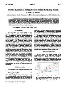
Figure 1: Relation among epidemic models, Lotka-Volterra models, and population dynamics models. Population dynamics is the branch of life sciences that studies short- and long-term changes in the size and age composition of populations, and how the biological and environmental processes influence those changes. In the past, most models for biological population dynamics have been of interest only in mathematical biology [64, 65]. Today, these models are adapted and applied in many more areas of science [66, 67]. Here below, models of knowledge dynamics will be of interest as bases of epidemic models. Such models are nowadays used because some stages of idea spreading processes within a population (e.g, of scientists), possess properties like those of epidemics. The mathematical modeling of epidemic processes has attracted much attention since the spread of infectious diseases has always been of great concern and considered to be a threat to public health [68, 69, 70]. In the history of science and society, many examples of ideas spreading seem to 10

occur in a way similar to the spread of epidemics. Examples of the former field pertain to the ideas of Newton on mechanics and the passion for ”High Critical Temperature Superconductivity” at the end of the twentieh century. Examples of the latter field are the spreading of ideas from Moses or Buddha [71], or discussions based on the Kermack-McKendrick model [72] for the epidemic stages of revolutions or drug spreading [73]. Epidemic models belong to a more general class of Lotka-Volterra models used in research on systems in the fields of biological population dynamics, social dynamics, and economics. The models can also be used for describing processes connected to the spread of knowledge, ideas and innovations (see Fig. 1). Two examples are the model of innovation in established organizations [74] and the Lotka-Volterra model for forecasting emerging technologies and the growth of knowledge [36]. In social dynamics, the Lanchester model of war between two armies can be mentioned, a model which in the case of reinforcements coincides with the Lotka-Volterra-Gause model for competition between two species [75]. Solomon and Richmond [76, 77] applied a Lotka-Volterra model to financial markets, while the model for the trap of extinction can be applied to economic subjects [78]. Applications to chaotic pairwise competition among political parties [79] could also be mentioned. To start the discussion of population dynamics models as applied to the growth of scientific knowledge with special emphasis on epidemic models, two kinds of models can be discussed (Fig. 2): (1) deterministic models, see Sec. 3, appropriate for large and small populations where the fluctuations are not drastically important, (2) stochastic models, see Sec. 4, appropriate for small populations. In the latter case the intrinsic randomness appears much more relevant than in the former case. Stochastic models for large populations will not be discussed. The reason for this is that such models usually consist of many stochastic differential equations, whence their evolution can be investigated only numerically. Finally, let us mention that the knowledge diffusion is closely connected to the structure and properties of the social network where the diffusion happens. This is a new and very promising research area. For example, a combination can be made between the theory of information diffusion and the theory of complex networks [80]. For more information about the relation between networks and knowledge, see the following chapters of the book.

11

Figure 2: Relationships between system size, influence of fluctuations, and discussed classes of models.

3

Deterministic models

Below, 13 selected deterministic models (see Fig. 3) are discussed. The emphasis is on models that can be used for describing the epidemic stage of the diffusion of ideas, knowledge, and technologies.

3.1

Logistic curve and its generalizations

In a number of cases, the natural growth of autonomous systems in competition can be described by the logistic equation and the logistic curve (S-curve) [81]. In order to describe trajectories of growth or decline in socio-technical systems, one generally applies a three-parameter logistic curve: N (t) =

K 1 + exp[−αt − β]

(1)

where N (t) is the number of units in the species or growing variable to study; K is the asymptotic limit of growth; α is the growth rate which specifies the ”width” of the S-curve for N (t); and β specifies the time tm when the curve 12

Figure 3: Discrete (3) and continuous (10) models discussed in the chapter. Two continuous models account for the influence of time lag, three models are simple models of technological diffusion. Two models are simple epidemic models and two models are more complicated models. In addition, the basic logistic curve is discussed. reaches the midpoint of the growth trajectory, such that N (tm ) = 0.5 K. The three parameters, K, α, and β, are usually obtained after fitting some data [82]. It is well known that many cases of epidemic growth can be described by parts of an appropriate S-curve. As an example, recall that the S-curve was also used for describing technological substitution [34, 83, 84], ca. 60 years ago. However, different interaction schemes can generate different growth patterns for whatever system species are under consideration [85]. Not every interaction scheme leads to a logistic growth [86]. The evolution of systems in such regimes may be described by more complex curves, such as a combination of two or more simple three-parameter functions [81, 87].

13

3.2

Simple epidemic and Lotka-Volterra models of technology diffusion

As recalled here above, the simplest epidemic models could be used for describing technology diffusion, like considering two populations/species: adopters and non-adopters of some technology. Such models can be put into two basic classes: either broadcasting (Fig. 4) or word-of-mouth models (Fig. 5). In the broadcasting models, the source of knowledge about the existence and/or characteristics of the new technology is external and reaches all possible adopters in the same way. In the word-of-mouth models, the knowledge is diffused by means of personal interactions. (1) The broadcasting model (Fig. 4) Let us consider a population of K potential adopters of the new technology and let each adopter switch to the new technology as soon as he/she hears about its existence (immediate infection through broadcasting). The probability that at time t a new subject will adopt the new technology is characterized by a coefficient of diffusion κ(t) which might or might not be a function of the number of previous adopters. In the broadcasting model κ(t) = a with (0 < a < 1); this is considered to be a measure of the infection probability. Let N (t) be the number of adopters at time t. The increase in adopters for each period is equal to the probability of being infected, multiplied by the current population of non-adopters [88]. The rate of diffusion at time t is dN = a[K − N (t)]. (2) dt The integration of (2) leads to the number of adopters: i.e., N (t) = K[1 − exp(−at)].

(3)

N (t) is described by a decaying exponential curve. (2) Word-of-mouth model (Fig. 5) In many cases, however, the technology adoption timing is at least an order of magnitude slower than the time it takes for information spreading [89]. This requires another modelization than in (1): the word-of-mouth diffusion model. Its basic assumption is that knowledge diffuses by means of face-toface interactions. Then the probability of receiving the relevant knowledge needed to adopt the new technology is a positive function of current users 14

Figure 4: Schematic representation of a broadcasting model of technology diffusion. The number of adopters of technology increases by mass media influence. N (t). Let the coefficient of diffusion κ(t) be bN (t) with b > 0. The rate of diffusion at time t is dN = b N (t) [K − N (t)] . (4) dt Then K   N (t) = (5) 0 −bK(t−t0 ) 1 + K−N e N0 where N0 = N (t = t0 ). N (t) is described by an S-shaped curve. A constraint exists in the word-of-mouth model: it explains the diffusion of an innovation not from the date of its invention but from the date when some number, N (t) > 0, of early users have begun using it. 15

Figure 5: Schematic representation of a word-of-mouth model of technology diffusion. The number of adopters of technology increases by interpersonal interactions. (3) Mixed information source model (Fig. 6) In the mixed information source model, existing non-adopters are subject to two sources of information (Fig. 6). The coefficient of diffusion is supposed to look like a + bN (t). The model evolution equation becomes dN = (a + bN (t)) [K − N (t)]. dt

(6)

The result of Eq.(6) is a (generalized) logistic curve whose shape is determined by a and b [88]. (4) Time lag Lotka-Volterra model of innovation diffusion (Fig. 7) Let it be again assumed that the diffusion of innovation in a society is accounted for by a combination of two processes: a mass-mediated process 16

Figure 6: Schematic representation of mixed information source model. The number of adopters increases by mass media influence and interpersonal contacts. and a process connected to interpersonal (word-of-mouth) contacts. Let N (t) be the number of potential adopters. Some of the potential adopters adopt the innovation and become real adopters. The equation for the the rate of growth of the real adopters n(t), in absence of time lag, is dn(t) = α[N (t) − n(t)] + βn(t)[N (t) − n(t)] − µn(t), dt

(7)

where α denotes the degree of external influence such as mass media, β accounts for the degree of internal influence by interpersonal contact between adopters and the remaining population; µ is a parameter characterizing the 17

Figure 7: Schematic representation of a Lotka-Volterra model with time lag. The model accounts for the time lag between hearing about innovation and its adoption. decline in the number of adopters because of technology rejection for whatever reason. A basic limitation in most models of innovation diffusion has been the assumption of instantaneous acceptance of the new innovation by a potential adopter [88, 90]. Often, in reality, there is a finite time lag between the moment when a potential adopter hears about a new innovation and the time of adoption. Such time lags usually are continuously distributed [91, 92]. The time lag between the knowledge about the innovation and its adoption can be captured by a distributed time lag approach in which the effects of time delays are expressed as a weighted response over a finite time interval through appropriately chosen memory kernels [93] (see Fig. 7). Whence

18

Eq.(7) becomes Z t dn(t) = α dτ K1∗ (t − τ ) [N (τ ) − n(τ )] + dt 0

β

Z t 0

dτ K2∗ (t − τ )n(τ )[N (τ ) − n(τ )] − µ

Z t 0

dτ K3∗ (t − τ )n(τ ).

(8)

Eq.(8) reduces to Eq.(7) when the memory kernels Ki∗ (t) (i = 1, 2, 3) are replaced by delta functions. Two generic types of kernels are usually considered [92]: K ∗ (t) = ν e−νt K ∗ (t) = ν 2 t e−νt ,

(9) (10)

in which ν −1 is some characteristic time scale of the system. The number of potential adopters N (t) changes over time. Several possible functional forms of N (t) are used [94]: N (t) = N0 (1 + at);

N0 > 0, a > 0

N (t) = N0 exp[gt]; N0 > 0, g > 0

(11) (12)

b ; 1 + d exp(−ct)

b > 0, d > 0, c > 0

(13)

N (t) = b − q exp(−rt);

b > 0, q > 0, r > 0.

(14)

N (t) =

Eq.(12) represents an approximation for short- and medium-term forecasting since for t large, N (t) grows without bound, as in Keynes [95]. Eqs.(13) and (14) are useful in long-term forecasting as N (t) has an upper limit. Such forms for N (t) are valid within a deterministic framework. However, a stochastic framework (see below) is more appropriate when the carrying capacity N (t) is governed by some stochastic process, as when the influence of socioeconomic and natural factors are subject to ”random” or hardly explainable fluctuations. In such systems, N (t) can be timedependent: for example, N (t) ∼ N0 (1 +  cos(ωt)) where  0. Then S>

γ − ν/I =ρ β

(21)

is the threshold density of susceptibles, i.e., no epidemics can develop from time t0 unless S0 , the number of susceptibles at that time, exceeds the threshold ρ: the epidemic state cannot be maintained over some time interval unless the number of susceptibles is larger than ρ through that interval of time. As I increases, ν/I converges to 0 and ρ converges rapidly to γ/β. In [71], Goffman evaluated the rate of change of infectives ∆I/∆t. From the system equations, it is difficult to determine I(t). Yet in the epidemic stage, the behaviour of I(t) is exponential. For small t close to t0 , I(t) can be expanded into a power series: I(t) = C0 + C1 t + C2 t2 + . . . Cn tn + . . . such that the approximate rate of ∆I/∆t can be obtained. On the basis of this rate and the raw data, the development and peak of some research activity can be predicted, - under the assumption that the research is in an epidemic stage. (2) SEIR model for the spreading of scientific ideas (Fig. 10) The SIR epidemic models can be further refined by introducing a fourth class, E, i.e., persons exposed to the corresponding scientific ideas (Fig. 10). Such models are discussed in [106, 107]; they belong to the class of so-called SEIR epidemic models. One typical model goes as follows βSI dE βSI ρEI dS = λN − ; = − κE − ; dt N dt N N ρEI dR dI = κE + − γI; = γI dt N dt

(22) (23)

where S(t) is the size of the susceptible population at time t, E(t) is the size of the exposed class, I(t) is the size of the infected class. These individuals have adopted the new scientific idea in their publications. Finally, R(t) is the size of the population of recovered scientists, i.e., those who no longer publish on the topic. The size of the entire population is: N = S +E +I +R. An exit term is assumed to be very small, and because of this, t is included in the recovered class. N grows exponentially with rate λ. The parameters of the model are: β, the probability and effectiveness of a contact with an adopter; 1/κ, the standard latency time, (in other words, the average duration of time after one has been exposed but before one includes the new idea in one’s own 24

Figure 10: SEIR model of intellectual infection with influxes of susceptibles and infectives to the corresponding scientific ideas, thus extending the SIR model by including a class of scientists exposed (E) to the specific scientific ideas. publication); 1/γ, the duration of the infectious period, thus how long one publishes on the topic and teaches others; ρ, the probability that an exposed person has multiple effective contacts with other adopters. This simple model can incorporate a wide range of behaviors. For many values of the parameters λ,β, κ, γ and ρ, the infected class grows as a logistic curve. For large values of the contact rate β or recruitment λ, I(t) grows nearly linearly, as indeed has been found empirically for some research fields [106].

25

FOR POLICY-MAKERS Take away box Nr.9: Epidemic models are the best suited for describing the expansion stage of a process growth.

(3) SI discrete model for the change in the number of authors in a scientific field (Fig. 11) With the goal of predicting the spreading out of scientific objects (such as

Figure 11: Schema of a discrete SI evolution model of the number of authors of scientific papers. The model takes into account that several scientists stop their work in a scientific field; it can be due to different reasons as for example death or losing interest in particular questions. theories or methods), Nowakowska [108] discussed several epidemic discrete models for predicting changes in the number of publications and authors in a given scientific field. With respect to the publications, the main assumption 26

of the models is that the number of publications in the next period of time (say, one year) will depend: (i) on the number of papers which recently appeared, and (ii) on the degree at which the subject has been exhausted. The numbers of publications appearing in successive periods of time should first increase, then would reach a maximum, and as the problem becomes more and more exhausted, the number of publications would decrease. Let it be assumed (Fig. 11) that if at a certain moment t the epidemics state is (xt , yt ) (xt is the number of infectives (authors who write papers on the corresponding research problems) , yt is the number of susceptibles), then for a sufficiently short time interval ∆t, one may expect that the number of infectives xt+∆t will be equal to xt − axt ∆t + bxt yt ∆t, while the number of susceptibles yt+∆t will be equal to yt − bxt yt ∆t; a and b being appropriate constants. Let the expected number of individuals who either die or recover, during the interval (t, t + ∆t), be axt ∆t, and let bxt yt ∆t be the expected number of new infections. The equations of this model are: xt+∆t = axt − axt ∆t + bxt yt ∆t yt+∆t = yt − bxt yt ∆t.

(24) (25)

Note here that such discrete models are useful for the analysis of realistic situations where the values of the quantities are available at selected moments (every month, every year, etc.). (4) Daley discrete model for the population of papers (Fig. 12) Daley [109] investigated the spread of news as follows: individuals who have not heard the news are susceptible and those who heard the news are infective. Recovery is not possible, as it is assumed that the individuals have perfect memory and never forget. The Daley model can be applied also to the population of papers [108] (see Fig. 12). For ∆t = 1 (year), the Daley model equation reads xt+1 = bxt N −

t X

!

xi

(26)

i=1

where x1 , x2 .... are the numbers of papers on the subject which appear in successive periods of time, b and N being parameters. The expected number xt+1 of papers in year t + 1 is proportional to the number xt of papers which P appeared in year t, and to the number N − x1 − x2 . . . − xt = N − ti=1 xi . N is the number of papers which have to appear in order to exhaust the 27

Figure 12: Daley model for evolution of population of papers on problems in a scientific field. The exhausting of the scientific field is taken into account. problem: the problem under consideration may be partitioned into N subproblems, such that solving any of them is worth a separate publication; these subproblems are solved successively by the scientists. The b and N parameters may be estimated by the method of least squares, e.g. from a given empirical histogram. A parameter characterizing the initial growth dynamics in the number of publications can also be introduced: τ = bN . Therefore, Eq.(26) can be used for short-time prediction, even when the corresponding research field is in the epidemic stage of its evolution. (5) Discrete model coupling the populations of scientists and papers (Fig. 13) A discrete model coupling the populations of scientists and papers can be considered (Fig. 13); it depends on four parameters: N , a, b and c. N as above denotes the number of sub-problems of the given problem; a is the probability that a scientist working on the subject in a given year abandons research on the subject for whatever reasons; b is the probability of obtaining

28

Figure 13: Discrete model for the joint evolution of populations of scientists and papers. The attractiveness of the field, the exhaustion of the field, and the possibility for declining interest for working in the scientific field are taken into account through adequate rate parameters. a solution to a given subproblem by one scientist during one year of research; c denotes the coefficient of attractiveness of the subject. The basic variables of the model are: ut , the number of scientists working on the subject in year t, and xt , the number of publications on the subject which appear in year t. The model equations are ut+1 = (1 − a)ut + cxt xt+1 = [1 − (1 − b)ut ] N −

(27) t X

!

xi .

(28)

i=1

The equation for the number ut+1 of scientists working on the subject in year t + 1 tells that in year t + 1, the expected number of scientists working on the 29

subject will be the number of scientists working on the subject in year t, ut , minus the expected number of scientists who stopped working on the subject, aut , plus the expected number of scientists, cxt , who became attracted to the problem by reading papers which appeared in year t. The equation expressing the number of publications in year t + 1 tells us that xt+1 equals the number of subproblems that were solved in the year t. The probability that a given subproblem will be solved in year t by a given scientist equals b. Then the probability of the opposite event, i.e. a given scientist will not solve a particular problem, equals 1 − b. As there are ut scientists working on the subject in year t, the probability that a given subproblem will not be solved by any of them is (1 − b)ut . Consequently, the probability that a given subproblem will be solved in year t (by any of the ut scientists working on the P subject) is equal to 1 − (1 − b)ut . Next, in year t there remained N − ti=1 xi subproblems to be solved. The expected number of subproblems solved in year t is equal to the product which gives the right-hand side of Eq.(28). N.B. It is assumed, that the waiting time for publishing of the paper is one year. A more realistic picture would be to assume that the unit of time is not one year, but two years, or that the publication has some other time delay. FOR POLICY-MAKERS Take away box Nr.10: In many cases, the data is available as one value per week, or one value per month, or one value per three months, etc. For modeling and subsequent short-range forecasting, so-called discrete (time) models are thus very appropriate.

3.5

Continuous models of the joint evolution of scientific sub-systems

(1) Coupled continuous model for the populations of scientists and papers: Goffman-Newill model The Goffman-Newill model [105] (Fig. 14) is based on the idea that the spreading process within a population can be studied on the basis of the literature produced by the members of that population. There is a transfer of infectious materials (ideas) between humans by means of an intermediate 30

Figure 14: Schema of Goffman-Newill model for the evolution of a scientific field. Scientists are attracted to a sub-field after being intellectually infected by papers from the sub-field. host (a written article). Let a scientific field be F and SF a sub-field of F . Let the number of scientists writing papers in the field F at t0 be N0 and the number of scientists writing papers in SF at t0 (the number of infectives) be I0 . Thus, S0 = N0 − I0 is the number of susceptibles; there is no removal at t0 , but there is removal R(t) at later times t. The number of papers produced on F at t0 is N00 and the number of papers produced in SF at this time is I00 . The process of intellectual infection is as follows: (a) a member of F is infected by a paper from I 0 ; (b) after some latency period, this infected member produces ’infected’ papers in N 0 , i.e. the infected member produces a paper in the subfield SF citing a paper from I 0 ; (c) this ’infected’ paper may infect other scientists from F and its sub-fields, such that the intellectual infection spreads from SF to the other sub-fields of F . Let β be the rate at which the susceptibles from class S become ’intel31

lectually infected’ from class I. Let β 0 be the rate at which the papers in SF are cited by members of N who are producing papers in SF . As the infection process develops, some susceptibles and infectives are removed, i.e. some scientists are no longer active, and some papers are not cited anymore. Let γ and γ 0 be the rates of removal of infectives from the populations I and I 0 respectively, and δ and δ 0 be the rates of removal from the populations of susceptibles S and S 0 . In addition, there can be a supply of infectives and susceptibles in N and N 0 . Let the rates of introduction of new susceptibles be µ and µ0 , i.e. the rates at which the new authors and new papers are introduced in F , and let the rates of introduction of new infectives be υ and υ 0 , i.e. the rates at which new authors and new papers are introduced in SF . In addition, within a short time interval a susceptible can remain susceptible or can become an infective or be removed; the infective can remain an infective or can become a removal; and the removal remains a removed. The immunes remain immune and do not return to the population of susceptibles. If, in addition, the populations are homogeneously mixed, the system of model equations reads dI dS = −βSI 0 − δS + µ; = βSI 0 − γI + υ dt dt dS 0 dR = γI + δS; = −β 0 S 0 I − δS 0 + µ0 dt dt dR0 dI 0 = β 0S 0I − γ 0I 0 + υ0; = γ 0I 0 + δ0S 0 dt dt

(29) (30) (31)

The conditions for development of an epidemic are as follows. If as an initial condition at t0 , a single infective is introduced into the populations N0 and N00 , then for an epidemic to develop, the change of the number of infectives 0 0 and ρ0 = γ β−υ must be positive in both populations. Then, for ρ = γ−υ 0 , β the threshold for the epidemic arises from the conditions βSI 0 > γI − υ and β 0 S 0 I 0 > γ 0 I 0 − υ 0 , such that the threshold is S0 S00 > ρρ0 .

(32)

The development of epidemics is given by the equation dI = D(t). The peaks dt d2 I of the epidemic occur at time points where dt2 = 0, while the epidemic’s size is given by I(t → ∞). (2) Bruckner-Ebeling-Scharnhorst model for the growth of n subfields in a scientific field 32

Figure 15: Schema of Bruckner-Ebeling-Scharnhorst model of evolution of n scientific sub-fields. Self-reproduction and decline of subfields as well as field mobility are taken into account. The evolution of growth processes in a system of scientific fields can be modeled by complex continuous evolution models. One of them, the BrucknerEbeling-Scharnhorst approach [110] (Fig. 15), is closely related to several generalizations of Eigen’s theory of prebiotic evolution and is briefly discussed here (see also [111]). In 1912, Lotka [112] published the idea of describing biological epidemic processes, like malaria, as well as chemical oscillations, with the help of a set of differential equations. These equations, known as Lotka-Volterra equations [113, 114], are used to describe a coupled growth process of populations. However, they do not reflect several essential properties of evolutionary processes such as the creation of new structural elements. Because of this, one has to consider a more general set of equations for the change in the number xi of the scientists from the i-th scientific subfield (a Fisher-Eigen-Schuster kind of model), i.e., n n X X dxi = (Ai − Di )xi + (Aij xj − Aji xi ) + Bij xi xj − k0 xi , dt j=1;j6=i j=1;j6=i

33

i, j = 1, . . . , n.

(33)

The model based on Eq.(33) describes the coupled growth of n subfields, of a scientific discipline. Three fundamental processes of evolution are included in Eq.(33) : (a) self-reproduction: students and young scientists join the field and start working on corresponding problems. Their choice is influenced mainly by the education process as well as by individual interests and by existing scientific schools; (b) decline: scientists are active in science for a limited number of years. For different reasons (for example, retirement) they stop working and leave the system; (c) field mobility: individuals turn to other fields of research for various reasons or maybe open up new ones themselves. The reasoning to obtain Eq.(33) goes as follows. The general form of the law for growth of the i-th subfield is supposed to be dxi = fi (~x), dt

~x = (x1 , ..., xn ).

(34)

By separation, fi = wi xi , one obtains the replicator equation dxi = wi xi , dt

i = 1, 2, . . . , n.

(35)

Notice that when wi = const, the fields are uncoupled, i.e., there is an exponential growth in science. Otherwise, wi itself is a function of x and of various parameters, but can be separated into three terms according to the above model assumptions , i.e., wi = Ai − Di +

n X j=1,j6=i

xj Aij − Aij . xi





(36)

Eq.(33) is thus obtained from Eq.(35) and Eq.(36) for Bij = 0, k0 = 0. To adapt this model to real growth processes, it can be assumed that the coefficients Ai , Di , and Aij themselves are functions of xi : Ai = A0i + A1i xi + . . . ; Di = Di0 + Di1 xi + . . . ; Aij = A0ij + A1ij xj + . . . (37) Each of the three fundamental processes of change is represented in Eq.(33) with a linear and a quadratic term only. For example, the terms A1i and Di1 account for cooperative effects in self-reproduction and decline processes 34

respectively, while Di0 accounts for a decline, because of aging. The contributions A0ij assume a linear type of field mobility behavior for scientists analogous to a diffusion process. On the other hand, the terms A1ij represent a directed process of exchange of scientists between fields. The best way to obtain these parameters is to estimate them for specific data bases using the method of least squares.

FOR POLICY-MAKERS Take away box Nr.11: The Bruckner-Ebeling-Scharnhorst model does not belong to the class of epidemic models which are best applicable only for describing the expansion stage of a process. The Bruckner-Ebeling-Scharnhorst model is an evolution model: it describes all stages of the evolution of a system.

4

Small-size scientific and technological systems. Stochastic models (Fig. 16)

Figure 16: Hierarchy of stochastic models discussed in this chapter. 35

The movement of large bodies in mechanics is governed by deterministic laws. When the body contains a small number of molecules and atoms, stochastic effects such as the Brownian motion become important. In the area of scientific systems, the fluctuations become very important when the number of scientists in a certain research subfield is small. This is typical for new research fields with only a few researching scientists. Several examples of stochastic models for the description of the diffusion of ideas or technology and the evolution of science are: (a) the model of evolution of scientific disciplines with an example pertaining to the case of elementary particles physics [115]; (b) stochastic models for the aging of scientific literature [116]; (c) stochastic models of the Hirsch index [55] and of instabilities in evolutionary systems [117]; (d) models of implementation of technological innovations [118], etc. [119]. In the following, see Fig. 16, two probabilistic and two stochastic models are discussed. Some attention is devoted to the master equation approach as well.

4.1

Probabilistic SI and SEI models

Epidemiological models of differential-equation-based compartmental type have been found to be limited in their capacity to capture heterogeneities at the individual level and in the interaction between individual epidemiological units [120]. This is one of the reasons to switch from models in which the number of individuals are in given known states to models involving probabilities. One such model [121] captures the diffusion of topics over a network of connections between scientific disciplines, as assigned by the ISI Web of Science’s classification in terms of Subject Categories (SCs). Each SC is considered as a node of a network along with all its directed and weighted connections to other nodes or SCs [121, 122]. As with epidemic models, nodes can be characterized in a medical way. SCs that are susceptible (S) are either not aware of a particular research topic or, if aware, may not be ready to adopt it. Incubating SCs (E) are those that are aware of a certain topic and have moved to do some research on problems connected with this topic. Infected SCs (I) are actively working and publishing in a particular research topic. Two probabilistic models, i.e., (i) the Susceptible-Exposed-Infected (SEI) model (Fig. 17) and (ii) a simpler Susceptible-Infected (SI) model (Fig. 18), are thereby only discussed. (1) Susceptible-Exposed-Infected (SEI) model 36

The SEI model equations for the evolution of the node state probabilities

Figure 17: Schema of the probabilistic SEI model for epidemics in a network connecting scientific disciplines. are given by [121]: X dSi (t) =− Aji Ij (t)Si (t), dt j

dEi (t) X = Aji Ij (t)Si (t) − γEi (t), dt j

(38)

(39)

dIi (t) = γEi (t), (40) dt where 0 ≤ Ii (t) ≤ 1 denotes the probability of node i being infected at time t (likewise for Si (t) and Ei (t)). The directed and weighted contact network 37

is represented by Aij = rΓij with Γij = (wij )i,j=1,...,N denoting the adjacency matrix that includes weighted links; r is the transmission rate per contact and 1/γ is the average incubation or latent period. This set of equations states that an increase in the probability Ei of a node i being exposed to an infection is directly proportional to the probability Si of node i being susceptible and the probability Ij of neighbouring nodes j being infected. The number of such contacts and the per-contact rate of transmission are incorporated in Aij . Likewise, Ei decreases if exposed/infected nodes become infected after an average incubation time 1/γ. The number of infected SCs at time t, according to the model, can be estiP mated as I(t) = i Ii (t). Since Si (t) + Ei (t) + Ii (t) = 1, for each t > 0, Eqs. (38) - (40) are readily understood, in view of Eq.(39). (2) Susceptible-Infected (SI) model The above SEI model can be simplified to an SI model when the possibility

Figure 18: Schema of the probabilistic SI model for epidemics in a network connecting scientific disciplines. of an exposed period is excluded, i.e,. if

38

dEi (t) dt

= 0. The equations for this

simpler SEI model are reduced to X dSi (t) =− Aji Ij (t)Si (t); dt j

dIi (t) X = Aji Ij (t)Si (t), dt j

(41)

where the probability Ii of a node i being infected and infectious only depends on the probability Si of the node i being susceptible. The comparison of both models with available data shows [121] that while the agreement at the population level is usually much better for the SEI model, for the same pair of parameters, the agreement at the individual level is better when the simpler SI model is used.

4.2

Master equation approach

(1) Stochastic evolution model with self-reproduction, decline, and field mobility There exists a high correlation between field mobility processes and the emergence of new fields [110]. This can be accounted for by a stochastic model (see Fig. 19), in which the system at time t is characterized by a set of integers N1 , N2 , ..., Ni , ..., Nn , with Ni being, e.g., the number of scientists working in the subfield i, which is considered now as a stochastic variable. The three fundamental types of scientific change mentioned in the discussion of the Bruckner-Ebeling-Scharnhorst model (see above) here correspond to three elementary stochastic processes with three different transition probabilities: • (a) For self-reproduction, the transition probability is given by W (Ni + 1 | Ni ) = A0i Ni = A0i Ni + A1i Ni (Ni − 1); • (b) The transition probability for decline is W (Ni − 1 | Ni ) = Di0 Ni + Di1 Ni (Ni − 1); • (c) The transition probability for field mobility is W (Ni + 1, Nj − 1 | Ni Nj ) = A0ij Nj + A1ij Ni Nj . The probability density P (N1 , . . . , Ni , Nj , . . . , t) is given by the so-called master equation ∂P = WP (42) ∂t which can be solved analytically only in some very special cases [123]. 39

Figure 19: Schema of the master equation model of evolution of scientific fields in presence of self-reproduction, decline, and field mobility. (2) The master equation as a model of scientific productivity The productivity factor is a very important ingredient in mathematically simulating a scientific community evolution. One way to model such an evolution is through a dynamic equation which takes into account the stochastic fluctuations of scientific community members productivity [127] (Fig. 20). The main processes of scientific community evolution accounted for by this model are, beside the biological constraints (like the self-reproduction, aging of scientists, and death), their departure from the field due to mobility or abandon of research activities. Call a the age of an individual and let a scientific productivity index ξ be in incorporated into the individual state space; both a and ξ are being considered to be continuous variables with values in [0, ∞]. The scientific community dynamics is described by a number

40

Figure 20: Schema of the master equation model for scientific productivity. density function n(a, ξ, t), - another form of scientific landscape, which specifies the age and productivity structure of the scientific community at time t. For example, the number of individuals with age inR [a1R, a2 ] and scientific productivity in [ξ1 , ξ2 ] at time t is given by the integral aa12 ξξ12 da dξ n(a, ξ, t). A master equation for this function n(a, ξ, t) can be derived [127]: ∂ ∂ + ∂a ∂t

!

n(a, ξ, t) = −[J(a, ξ, t) + w(a, ξ, t)] n(a, ξ, t) + Z ξ

dξ 0 χ(a, ξ − ξ 0 , t) n(a, ξ − ξ 0 , t),

(43)

−∞

where w(a, ξ, t) denotes the departure rate of community members. If x(t) is a random process describing the scientific productivity variation and if 41

pa (x, t | y, τ ) (with τ < t) is the transition probability density corresponding to such a process, then pa (ξ + ξ 0 , t + ∆t | ξ, t) . (44) χ(a, ξ, ξ , t) = lim ∆t→0 ∆t The transition rate, atR time t from the productivity level ξ, J(a, ξ, t) is by ∞ definition: J(a, ξ, t) = −ξ dξ 0 χ(a, ξ, ξ 0 , t). The increment ξ 0 may be positive or negative. The balance equation for n(a, ξ, t) reads as follows 0

n(a + ∆a, ξ, t + ∆t) = n(a, ξ, t) − J(a, ξ, t) n(a, ξ, t) ∆t + "Z ξ

# 0

0

χ(a, ξ − ξ , t) n(a, ξ − ξ , t)dξ

0

∆t − w(a, ξ, t) n(a, ξ, t) ∆t.

(45)

−∞

The term on the right-hand side, [1 − J(a, ξ, t)∆t]n(a, ξ, t), describes the proportion of individuals whose scientific productivity does not change in [t, t + ∆t]; the integral term describes the individuals whose scientific productivity becomes equal to ξ because of increasing or decreasing in [t, t + ∆t]; the last term corresponds to the departure of individuals due to stopping research activities or death. After expanding n(a + ∆t, ξ, t + ∆t) around a and t, keeping terms up to the first order in ∆t, one obtains the master equation Eq.(43). As the master equation is difficult to handle for an elaborate analysis, it is often reduced to an approximated equation similar to the well-known Fokker-Planck equation [124, 125, 126]. The approximation goes as follows. Let Z ∞ 1 < (ξ 0 )k >; k = 1, 2, . . . , dξ 0 (ξ 0 )k χ(a, ξ, ξ 0 , t) = lim µk (a, ξ, t) = ∆t→0 ∆t −ξ (46) where the brackets denote the average with respect to the conditional probability density pa (ξ + ξ 0 , t + ∆t | ξ, t). In addition, the following assumptions are made: (i) µ1 , µ2 < ∞; µk = 0 for k > 3; (ii) n(a, ξ, t) and χ(a, ξ, ξ 0 , t) are analytic in ξ for all a, t and ξ 0 . The additional assumption µk = 0 for k > 3 demands the productivity to be continuous in the sense that as ∆t → 0, the probability of large fluctuations | ξ 0 | must decrease so quickly that → 0 more quickly than ∆t. When the above assumptions hold, the function n satisfies the equation [127]: ! ∂ ∂ ∂(µ1 n) 1 ∂ 2 (µ2 n) + + − wn. (47) n=− ∂a ∂t ∂ξ 2 ∂ξ 2 42

If w = 0, Eq.(47) is converted to the well known Fokker-Planck equation. Eq.(47) describes the scientific community evolution through a drift along the age component and a drift and diffusion with respect to the productivity component. The diffusion term characterized by the diffusivity µ2 takes into account the stochastic fluctuations of scientific productivity conditioned by internal factors (such as individual abilities, labour motivations, etc.) and external factors (such as labor organization, stimulation system, etc.). The initial and boundary conditions for Eq.(47) are: (a) n(a, ξ, 0) = n0 (a, ξ), where n0 (a, ξ) is a known function defining the community age and productivity distribution at time t = 0; and (b) n(0, ξ, t) = ν(ξ, t) where the function ν(ξ, t) represents the intensity of input flow of new members at age a = 0 being set ν(ξ, 0) = n0 (0, ξ). In addition, n(a, ξ, t) → 0 as a → ∞. The general solution of equation Eq.(47) with the above initial condition (a) and boundary condition (b) is still a difficult task. However, for many practical applications, a knowledge of first and second moments of distribution function n(a, ξ, t) is sufficient. Eq.(47) can be solved numerically or can be reduced to a system of ordinary differential equations [127].

FOR POLICY-MAKERS Take away box Nr.12: In deterministic cases, the system is robust against fluctuations: it follows some trajectory and the fluctuations are too weak to change it. When the fluctuations are important, then different trajectories for the evolution of the system become possible. To each trajectory, a probability can be assigned. This probability reflects the chance that the system will follow the corresponding trajectory. The collection of the probabilities leads to a probability distribution which can be calculated, in many evolutionary cases, on the basis of the master equation approach.

Finally, two additional problems that can be treated by the master equation approach can be mentioned: • Age-dependent models where the birth and death rates connected to the selection are age-dependent [128, 129] • The problem of new species in evolving networks [111]. On the basis of a stochastic treatment of the problem, the notion of ’innovation’ can 43

be introduced in a broad sense as a disturbance and/or an instability of a corresponding social, technological, or scientific system. The fate of a small number of individuals of a new species in a biological system can be thought to be mathematically equivalent to some extent to the fate of a new idea, a new technology, or a new model of behavior. The evolution of the new species can be studied on evolving networks, where some nodes can disappear and new nodes can be introduced. This evolution of the network can change significantly the dynamic behavior of the entire system of interacting species itself. Some of the species can vanish in a finite time. This feature can be captured effectively by the master equation approach.

5

Space-time models. Competition of ideas. Ideological struggle

A further level of complication is to include spatial variables explicitly in the above models describing the diffusion of ideas. At this stage of globalization of economies, with several of its concomitant features, like idea, knowledge, and technology diffusion, to consider the spatial aspect is clearly a must. A large amount of research on the spatial aspects of diffusion of populations is already available. As examples of early work, papers by Kerner [130], Allen [131], Okubo [132], and Willson and de Roos [133] can be pointed out. From the point of view of diffusion of ideas and scientists, the previously discussed continuous model of research mobility [110] has to be singled out. Moreover, the model presented below is closely connected to the space-time models of migration of populations developed by Vitanov and co-authors [134, 135]. In addition, a reproduction-transport equation model (see Fig. 21) can be discussed.

5.1

Model of competition between ideologies

The diffusion of ideas is necessarily accompanied by competition processes. One model of competition between systems of ideas (ideologies) goes as follows (Fig. 22). Let a population of N individuals occupy a two-dimensional plane. Suppose that there exists a set of ideas or ideologies P = {P0 , P1 , . . . , Pn } and let Ni members of the population be followers of the Pi ideology . The members N0 of the class P0 are not supporters of any ideology; in some 44

Figure 21: Relations between space-time models discussed in this chapter. sense, they have their own individual one and do not wish to be considered associated with another one, global or not. In such a way, the population is divided in n + 1 sub-populations of followers of different ideologies. The total population is: N = N0 + N1 + . . . Nn . Let a small region ∆S = ∆x∆y be selected in the plane. In this region there are ∆Ni individuals holding the i-th ideology, i = 0, 1, . . . , n. If ∆S is sufficiently small, the density of the i . i-th population can be defined as ρi (x, y, t) = ∆N ∆S Allow the members of the i-th population to move through the borders of the area ∆S. Let ~ji (x, y, t) be the current of this movement. Then (~ji ·~n)δl is the net number of members of the i-th population/ideology, crossing a small line δl with normal vector ~n. Let the changes be summarized by the function Ci (x, y, t). The total change of the number of members of the i-th population is ∂ρi + div~ji = Ci . (48) ∂t

45

Figure 22: Schema of the space-time model for describing competition between ideologies. The first term in Eq.(48) describes the net rate of increase of the density of the i-th population. The second term describes the net rate of immigration into the area. The r.h.s. of Eq.(48) describes the net rate of increase exclusive of immigration. Let us now specify ~ji and Ci : ~ji is assumed to be made of a non-diffusion (1) (2) (2) part ~ji and a diffusion part ~ji where ~ji is assumed to have the general form of a linear multicomponent diffusion [130] in terms of a diffusion coefficient Dik ~ji = ~jI(1) + ~j2(2) = ~ji(1) −

n X

Dik (ρi , ρk , x, y, t)∇ρk .

(49)

k=0

Let some of the followers of the ideology Pi be capable of and interested in changing ideology: i.e., they can convert from the ideology Pi to the ideology Pj . It can be assumed that the following processes can happen with respect to the members of the subpopulations of the property holders: (a) deaths: described by a term ri ρi . It is assumed that the number of 46

deaths in the i-th population is proportional to its population density. In general ri = ri (ρν , x, y, t; pµ ), where ρν stands for (ρ0 , ρ1 , . . . , ρN ) and pµ stands for (p1 , . . . , pM ) containing parameters of the environment; (b) noncontact conversion: in this class are included all conversions exclusive of the conversions by interpersonal contact between the members of whatever populations. A reason for non-contact conversion can be the existence of different kinds of mass communication media which make propaganda for whatever ideologies. As a result, members of each population can change ideology. For the i-th population, the change in the number of members is: Pn j=0 fij ρj , fii = 0. In general, fij = fij (ρν , x, y, t; pµ ); (c) contact conversion: it is assumed that there can be interpersonal contacts among the population members. The contacts happen between members in groups consisting of two members (binary contacts), three members (ternary contacts), four members, etc. As a result of the contacts, members of each population can change their ideology. For binary contacts, let it be assumed that the change of ideology probability for a member of the j-th population is proportional to the possible number of contacts, i.e., to the density of the i-th population. Then the total number of ”conversions” from Pj to Pi is aij ρi ρj , where aij is a parameter. In order to have a ternary contact, one must have a group of three members. The most simple is to assume that such a group exists with a probability proportional to the corresponding densities of the concerned populations. In a ternary contact between members of the i-th, j-th, and k-th population, members of the j-th and k-th populations can change their ideology according to Pi = bijk ρi ρj ρk , where bijk is a parameter. In general, aij = aij (ρν , x, y, t; pµ ); bijk = bijk (ρν , x, y, t; pµ ); etc. On the basis of the above, the Ci term looks as follows (for more research of these types of population models see [136, 137, 138]): Ci = ri ρi +

n X j=0

fij ρj +

n X

aij ρi ρj +

j=0

n X

bijk ρi ρj ρk + . . . ,

(50)

j,k=0

and the model system of equations becomes n n X X ∂ρi (1) ~ + divji − div(Dij ∇ρj ) = ri ρi + fij ρj + ∂t j=0 j=0 n X

aij ρi ρj +

j=0

n X

bijk ρi ρj ρk + . . .

(51)

j,k=0

The density of the entire population is ρ = 47

Pn

i=0

ρi . It can be assumed

that it changes in time according to the Verhulst law (but see the note after Eq.(56)!)   ρ ∂ρ = rρ 1 − (52) ∂t C where C(ρν , x, y, t; pµ ) is the so-called carrying capacity of the environment [96] and r(ρν , x, y, t; pµ ) is a positive or negative growth rate. When pertinent sociological data are available, the same type of equation could hold for any i-th population with a given ri . (i) (i) First, consider the case in which the current ~ji is negligible, i.e., ~ji ≈ 0 (no diffusion approximation). In addition, consider only the case when all parameters are constants. The model system of equations becomes n n n X X X ∂ρi aij ρi ρj + fij ρj + ∆ρj = ri ρi + − Dij ∂t j=0 j=0 j=0 n X

bijk ρi ρj ρk + . . . ,

(53)

j,k=0

for ∆=

∂2 ∂2 + , ∂x2 ∂y 2

i = 0, 1, 2, . . . , n.

(54)

Let plane-averaged quantities and fluctuations (linear or nonlinear) be enough relevant. Let q(x, y, t) be a quantity defined in an area S. By defiRR nition, a plane-averaged quantity is q = S1 S dxdy q(x, y, t). Call the fluctuations Q(x, y, t) such that q(x, y, t) = q(t) + Q(x, y, t). If the territory is large and within the stationary approximation, S can be assumed to be large enough such that each plane-averaged combination of fluctuations vanishes, suchR that Qi = Qi Qj = Qi Qj Qk = . . . = 0. In addition to S being R large and R R S dxdy∆Qk assumed to be finite, it can be also assumed that ∆Qk = S1 S dxdy∆Qk → 0. On the basis of the above (reasonable) assumptions, it is possible to separate the dynamics of the averaged quantities from the dynamics of fluctuations. As a result of the plane-average of Eq.(53), the following equations for the dynamics of the plane-averaged densities are obtained n X

dρ ρ ρ0 = ρ − ρi ; = rρ 1 − dt C i=1 

48



(55)

n n n X X X dρi = ri ρ i + bijk ρi ρj ρk + . . . fij ρj + aij ρi ρj + dt j=0 j=0 j,k=0

(56)

Instead of (55) we can write an equation for ρ0 from the kind of (56). Then the total population density ρ will not follow the Verhulst law. Equations (55) and (56) represent the model of ideological struggle proposed by Vitanov, Dimitrova and Ausloos [139]. There is one important difference between the Lotka-Volterra models [112, 114], often used for describing prey-predator systems, and the above model of ideological struggle. The originality resides in the generalization of usual prey-predator models to the case in which a prey (or predator) changes its state and becomes a member of the predator pack (or prey band), due to some interaction with its environment or with some other prey or predator. Indeed, it can be hard for rabbits and foxes to do so, but it can be often the case in a society: a member of one population can drop his/her ideology and can convert to another one. In order to show the relevance of such extra conditions on an evolution of populations, consider a huge (mathematical) approximation, - it might be a drastic one in particular in a country with a strictly growing total population. (Recall that the growth rate r could be positive or negative or time-dependent). Let r be > 0 and let the maximum possible population of the country be C. Consider more convenient notations by setting ρ = N ; ρ0 = N0 ; ρi = Ni and assume that the binary contact conversion is much stronger than the ternary, etc. conversions. The system equations become N = N0 +

n X i=1

dN N = rN 1 − dt C 

Ni ;

n n X X dNi bij Ni Nj . = ri Ni + fij Nj + dt j=0 j=0



(57)

(58)

Reduce the discussion of Eqs.(57) and (58) to a society in which there is the spreading of only one ideology; therefore, the population of the country is divided into two groups: N1 , followers of the ”invading” ideology and N0 , people who are at first ”indifferent” to this ideology. Let only the non-contact conversion scheme exist, as possibly moving the ideology-free population toward the single ideology; thus f10 is finite, but b10 = 0. Let the initial conditions be N (t = 0) = N (0) and N1 (t = 0) = N1 (0). The solution of the

49

system of model equations is N (t) =

CN (0) , N (0) + (C − N (0))e−rt

(59)

like the Verhulst law, but 

f10 − r1 Cf10 C − N (0) , 1, − Φ − − r N (0) r   C − N (0) f10 − r1 (60) e(f10 −r1 )t Φ − , 1, − N (0)ert r

N1 (t) = e−(f10 −r1 )t N1 (0) +

 



with N0 (t) = N (t) − N1 (t) P∞

(61) zn

in which Φ is the special function Φ(z, a, v) = n=0 (v+n)a ; | z |< 1. The obtained solution describes an evolution in which the total population N reaches asymptotically the carrying capacity C of the environment. The number of adepts of the ideology reaches an equilibrium value which ˆ1 = Cf10 /(f10 − r1 ) of the model equation corresponds to the fixed point N dN1 for dt . The number of people who are not followers of the ideology asympˆ1 . Let C = 1, f10 = 0.03, and r1 = −0.02, then totically tends to N0 = C − N ˆ N1 = 0.6, which means that the evolution of the system leads to an asymptotic state in which 60 % of the population are followers of the ideology and 40 % are not. Other more complex cases with several competing ideologies can be discussed, observing steady states or/and cycles (with different values of the time intervals for each growth or/and decay), chaotic behaviors, etc. [139]. In particular, it can be shown that accepting a slight change in the conditions of the environment can prevent the extinction of some ideology. After almost collapsing, some ideology can spread again and can affect a significant part of the country’s population. Two kinds of such resurrection effects have been found and described as phoenix effects in the case of two competing ideologies. In the phoenix effect of the first kind, the equilibrium state connected to the extinction of the second ideology exists but is unstable. In the phoenix effect of the so-called second kind, the equilibrium state connected to extinction of the second ideology vanishes. In fine, the above model seems powerful enough to discuss many realistic cases. The number of control parameters seems huge, but that is the case for many competing epidemics in 50

complex systems. However, it was observed that the values of parameters can be monitored when enough data is available, including the time scales [139].

FOR POLICY-MAKERS Take away box Nr.13: Space-time models are very appropriate for modeling migration processes such as the spatial migration of scientists, besides the diffusion of ideas through competition without strictly physical motion.

5.2

Continuous model of evolution of scientific subfields. Reproduction-transport equation

The change of subject of a scientist can be considered as a migration process [110, 140]. Let research problems be represented by sequences of signal words or macro-terms Pi = (m1i , m2i , . . . , mki , . . . , mni ) which are registered according to the frequency of their appearance, joint appearance, etc., respectively, in the texts. Each point of the problem space, described by a vector ~q, corresponds to a research problem, with the problem space consisting of all scientific problems (no matter whether they are under investigation or not). The scientists distribute themselves over the space of scientific problems with density x(~q, t). Thus, there is a number x(~q, t)d~q working at time t in the element d~q. The field mobility processes correspond to a density change of scientists in the problem space: instead of working on problem ~q, a scientist may begin to work on problem q~0 . As a result, x(~q, t) decreases and x(q~0 , t) increases. This movement of scientists (see also Fig. 23) can be described by means of the following reproduction-transport-equation: !

∂ ∂x(~q, t) ∂x(~q, t) = x(~q, t) w(~q | x) + f (~q, x) + D(~q) . ∂t ∂~q ∂~q

(62)

In Eq.(62), self-reproduction and decline are represented by the term w(~q | x) x(~q, t). For the reproduction rate function w(~q | x), one can write w(~q | x) = a(~q) +

Z

dq~0 b(~q, q~0 ) x(q~0 , t).

51

(63)

Figure 23: Schema of the reproduction-transport equation model of joint evolution of scientific fields. The local value of a(~q) is an expression of the rate at which the number of scientists on field ~q is modified through self-reproduction and/or decline, while b(~q, q~0 ) describes the influence exerted on the field ~q by the neighbouring field q~0 . The field mobility is modeled by means of the term  ∂ ∂ f (~q, x) + D(~q) ∂~ x(~q, t) . In most cases, Eq.(62) can only be solved nu∂~ q q merically. For more details on the model, see [110].

52

Figure 24: Statistical laws and their relationships as discussed in the chapter.

6

Statistical approaches to the diffusion of knowledge

Solomon and Richmond [76, 77] have shown that the systems of generalized Lotka-Volterra equations are closely connected to the Pareto-Zipf probability distribution. Since such a distribution arises among other distributions and laws connected to the description of the diffusion of knowledge, it is of interest to discuss briefly the diffusion of knowledge within statistical approach studies. Lotka was its pioneer; a large amount of research has followed. Just as examples, one can mention the work of Yablonsky and Haitun on the Lotka law for the distribution of scientific productivity and its connection with the Yule distribution [141, 142, 143], where the non-Gaussian nature of the scientific activities is emphasized. Interesting applications of the Zipf law are also presented in [144]. The connection to the non-Gaussian distributions concepts of self-similarity and fractality have been applied to the scientific 53

system in [145] and [146]. Several tools for appropriate statistical analysis are hereby discussed. At the center of the discussion Lotka law shall receive some special attention (see Fig. 24) 2 . As part of this discussion on the statistical approach, the analysis of the productivity of scientists can be considered. The information connected to new ideas is thought to be often codified in scientific papers. Thus, the statistical aspects of scientific productivity is of practical importance. For example, the Lotka law reflects the distribution of publications over the set of authors considered as the information sources. Bradford law describes the distribution of papers on a given topic over the set of journals publishing these papers and ranked according to the order in the decrease of the number of papers on a given topic in each journal. These laws have a non-Gaussian nature and, because of this, possess specific features such as a concentration and dispersal effect [141]: for example, it is found that there is a small number of highly productive scientists who write most of the papers on a given topic and, on the other hand, a large number of scientists with low productivity. In order to give an example of the connection between the deterministic and statistical approaches, remember that the Goffman-Newill model, discussed here above, presents a connection between the number of scientists working in a research area and the number of relevant publications. In [106], it was found that the number of new publications scale as a simple power law with the corresponding number of new authors: ∆P = C(∆T )α where ∆P and ∆T are the new publications and the new authors over some time period (for an example one year). C is a normalization constant, and α is a scaling exponent. It has been demonstrated [106] that the latter relationship provides a very good fit to data for six different research fields, but with different values of the scaling exponent α. For α > 1, a field would grow by showing an increase in the number of publications per capita, i.e., in such a research field, the individual productivity increases as the field attracts new scientists. A field with α < 1 has a per capita decrease in productivity. This can be a warning signal for a dying subject matter. It would be interesting to observe whether the exponent α is time-dependent, as is the case in related characterizing scaling exponents of financial markets [148] or in meteorology[149]. Policy control can thus be implemented for shaking α, 2

Let us mention a curious and interesting fact connected to statistical indicators. Very interesting is the conclusion in [147] that the scale-independent indicators show that in the fast growing innovation system of China, research institutions financed by the government play a more important role than the enterprises.

54

thus the field mobility. FOR POLICY-MAKERS Take away box Nr.14: There exist two different kinds of statistical approaches for the analysis of scientific productivity: (i) the frequency approach and (ii) the rank approach. The frequency approach is based on the direct statistical counting of the number of corresponding information sources, such as scientists or journals. The rank approach is based on a ranking of the sources with respect to their productivity. The frequency and the rank approaches represent different and complementary reflections of the same law and form.

6.1

Lotka law. Distributions of Pareto and Yule.

Pareto [150] formulated the 80/20 rule: it can be expected that 20% of people will have 80% of the wealth. Or it can be expected that 80% of the citations refer to a core of 20% of the titles in journals. The idea of the rule of Pareto is very close to the research of Lotka who noticed the following dependence for the number of scientists nk who wrote k papers nk =

n1 ; k = 1, 2, . . . , kmax . k2

(64)

In Eq.(64), n1 is the number of scientists who wrote just one paper and kmax is the maximal productivity of a scientist. kX max k=1

nk = n1

kX max k=1

1 =N k2

(65)

where N is the total number of scientists. If we assume that kmax → ∞ P 2 and take into account the fact that ∞ k=1 1/k = π/6, we obtain a limiting value for the portion of scientists with the minimal productivity (single paper authors) in the given population of authors: P1 = n1 /N ≈ 0.6. Then, if the left and the right hand sides of Eq.(64) are divided by N, the frequency P expression for the productivity distribution is: p1 = 0.6/k 2 ; ∞ k=1 pk = 1. Eq. (64) is called Lotka law, or the law of inverse squares: the number of scientists who wrote a given number of papers is inversely proportional to the square of this number of papers. 55

It must be noted that, like many other statistical regularities, Lotka law is valid only on the average since the exponent in the denominator of Eq.(64) is not necessarily equal to two [141]. Thus, Lotka law should be considered as the most typical among a more general family of distributions: nk =

n1 ; k 1+α

p1 =

p1

(66)

k 1+α

where α is the characteristic exponent of the distribution, n1 is the normalizing coefficient which is determined as follows: −1



max 1  n1 kX = p1 = α N k=1 1 + k

.

(67)

Then the distribution of scientific output, Eq.(66), is determined by three parameters: the proportion of scientists with the minimal productivity p1 , the maximal productivity of a scientist kmax , and the characteristic exponent α. If one of these parameters is fixed, it is possible to study the dependence between two others. Let us fix kmax in Eq.(67). Then, we obtain the proportion of ”single paper authors” p1 as a function of α: p1 (α). When Eq.(67) is differentiated with respect to α, one can show that the corresponding derivative is positive for any α : dp1 (α)/dα > 0. On the basis of a similar analysis of the portion of scientists with a larger productivity pk (α) as a function of α, we arrive at the conclusion: the increase of α is accompanied by the increase of low-productivity scientists. This means that when the total number of scientists is preserved the portion of highly productive scientists will decrease. Let us show that the Lotka law is an asymptotic expression for the Yule distribution. In order to obtain the Yule distribution, one considers the process of formation of a collection of publications as a Markov-type stochastic process. In addition, it is assumed that the probability of writing a new paper depends on the number of papers that have been already written by the scientist at time t: the probability of the transition into a new state on the interval [t, t + ∆t] should be a function of the state in which the system is at time t. Moreover, the probability of publishing a new paper during a time interval ∆t, p(x → x + 1, ∆t) is assumed to be proportional to the number x of papers that have been written by the scientists, introducing an intensity coefficient λ: p(x → x + 1, ∆t) ∝ λx∆t. After solving the corresponding system of differential equations for this process, the following expression (the 56

Yule distribution) for the probability p(x/t) of a scientist writing x papers during a time t is obtained [141]: p(x/t) = exp(−λt)(1 − exp(−λt))x−1 , x = 1, 2 . . .

(68)

The mean value of the Yule distribution is xt = exp(λt). Let us take into account the fact that every scientist works on a given subject during a certain finite random time interval [0, t] which depends on the scientist’s creative potential, the conditions for work, etc. With the simplest assumption that the probability of discontinuing work on a given subject is constant at any time, one obtains an exponential distribution for the time of work of any author in the scientific field under study: p(t) = µ exp(−µt), where µ is the distribution parameter. The time parameter t which characterizes the productivity distribution, Eq.(68), is a random number. Then in order to obtain the final distribution of scientific output observed in the experiment over sufficiently large time intervals, Eq.(68) should be averaged with respect to this parameter t which is distributed according to the exponential law: p(x) =

Z ∞

dt p(x/t)p(t) =

Z ∞

dt exp(−λt)(1−exp(−λt))µ exp(−µt). (69)

0

0

After integrating Eq.(69), the distribution of scientific output reads   µ µ (70) p(x) = B x, + 1 = αB(x, α + 1), x = 1, 2, . . . λ λ where B(x, α + 1) = Γ(x)Γ(αx + 1)/Γ(x + α + 1) is a Beta-function, Γ(x) ≈ (x−1)! is a Gamma-function, and α = µ/λ is the characteristic exponent. For instance, if α ≈ 1 then p(x) = 1/[x(x + 1)]. Let us assume that x → ∞ and apply the Stirling formula. Thus, the asymptotics of the Yule distribution Eq.(70) is like Lotka law Eq.(66) (up to a normalizing constant): p(x) ∝ Γ(α + 1)α/x1+α .

6.2

Pareto distribution, Zipf-Mandelbrot and Bradford laws

For large enough values of the total number of scientists and the total number of publications, we can make the transition from discrete to continuous representation of the corresponding variables and laws. The continuous analog of Lotka law, Eq. (66), is the Pareto distribution α p(x) = x0



x0 x

α+1

; 57

x ≥ x0 ; α > 0

(71)

which describes the distribution density for a number of scientists with x papers; x0 is the minimal productivity x0