Boosting Grammatical Inference with Confidence Oracles

Boosting Grammatical Inference with Confidence Oracles

Jean-Christophe Janodet [email protected] EURISE, Faculty of Sciences, 23 rue Paul Michelon, University of Jean Monnet, 42023 Saint-Etienne, FRANCE Richard Nock [email protected] DSI, Universit´e Antilles-Guyane, BP 7209, 97275 Schoelcher, FRANCE (Martinique) Marc Sebban [email protected] EURISE, Faculty of Sciences, 23 rue Paul Michelon, University of Jean Monnet, 42023 Saint-Etienne, FRANCE Henri-Maxime Suchier [email protected] EURISE, Faculty of Sciences, 23 rue Paul Michelon, University of Jean Monnet, 42023 Saint-Etienne, FRANCE

Abstract In this paper we focus on the adaptation of boosting to grammatical inference. We aim at improving the performances of state merging algorithms in the presence of noisy data by using, in the update rule, additional information provided by an oracle. This strategy requires the construction of a new weighting scheme that takes into account the confidence in the labels of the examples. We prove that our new framework preserves the theoretical properties of boosting. Using the state merging algorithm rpni∗ , we describe an experimental study on various datasets, showing a dramatic improvement of performances.

1. Introduction Grammatical inference is a subtopic of machine learning whose aim consists in learning models of languages (sets of words or sequences). Among them, deterministic finite automata (dfa) are finite state machines which take words as input, and accept or reject them according if they characterize or not the concept to learn. In machine learning, a dfa can be seen as a classifier which separates the set of all words in two classes, a positive one (for the accepted words) and a negative one (for the rejected words). A practical reason which explains the efforts made to learn such classifiers comes from the fact that many applications, Appearing in Proceedings of the 21 st International Conference on Machine Learning, Banff, Canada, 2004. Copyright 2004 by the authors.

e.g. speech recognition, pattern matching, language processing, etc., can take advantage of the structural and semantic properties of dfa (de la Higuera, 2004). Among the algorithms aiming at learning dfa, those based on state merging have been widely studied during the last decade, and particularly edsm (Lang et al., 1998) and the well known rpni (Oncina & Garc´ıa, 1992). Both of them learn from a sample E = E+ ∪E− , and try to infer, by state merging, a small dfa that accepts all the words of E+ (called positive examples), and rejects all those of E− (called negative ones). For instance, the dfa in Figure 1 was computed by rpni with E+ = {b, abb, ab, bab, λ} and E− = {aa, ba}, where λ denotes the empty string. A word is accepted if its parsing starts from the initial state 0, follows transitions, and ends in a final state (always positive and graphically described by a double circle). Notice that this is the case for all the elements of E+ ending in the unique final state 0. The negative words are rejected, i.e. their parsing do not reach a final state. b a 0

1 b

Figure 1. A dfa with two states and three transitions.

rpni is an exact learning algorithm because it fits the data. It is proven that if E contains some special (characteristic) words, then rpni is able to infer, in polynomial time, the dfa that produced the data (Oncina & Garc´ıa, 1992), called the target dfa. However, the specificities of modern databases, which

often contain noisy data, challenge these theoretical properties. Since rpni is not immune to overfitting, noisy data have dramatic effects, and penalize the dfa in terms of number of states and error rate. Noise tolerance in such algorithms is thus a crucial problem studied in grammatical inference, confirming the same trend as in the whole machine learning field. The first attempt to limit the risk of overfitting in state merging algorithms was proposed by Sebban and Janodet (2003); they tried to relax the merging rule of rpni without endangering the generalization error of the dfa. They introduced the new algorithm rpni∗ , whose merging rule, based on statistical inference theory, allows to tolerate the presence of noisy words. From an experimental standpoint, this yields a significant improvement over rpni’s performances. But their approach is doubly limited: first, they provide theoretical results showing difficulties to infer the target dfa for noise levels over 10%. Second, due to its statistical nature, the use of rpni∗ can result in a wrongly accepted merging. Actually, while rpni does not admit any negative example in a final state, positive and negative words can share the same final state with rpni∗ due to the relaxation of the merging constraint. While one hopes that such negative words are indeed noisy data, one can be afraid of accepting truly negative words, which would lead to serious problems. In fact, the underlying problem of rpni∗ has to be linked to a couple of recurrent questions in machine learning: (i) is it possible to optimize the performances of a learning algorithm (here a state merging one)? (ii) is it possible to control this optimization even in the presence of noisy data (that would avoid here to merge “true” negative and positive examples in the same state)? Indisputably, we think that both of these questions are a matter for boosting, despite the fact that it has never been adapted to dfa inference. The strategy of boosting, and its algorithm adaboost (Freund & Schapire, 1996; Freund & Schapire, 1997) (see Algorithm 1), consists in successively training T times a learning algorithm wl on various probability distributions wt over the learning sample E, and in combining the resulting classifiers ht (called weak hypotheses) in an efficient single classifier HT . At each round, the current distribution favors (exponentially) the weights of examples misclassified by the previous hypothesis. Some recent works tried to limit the risk of overfitting of boosting in the presence of noise by answering the following question: when does a misclassified example really deserve a weight increase? adaboost tending (wrongly) to exponentially increase the weight of the outliers, new approaches aim then at controlling

for all x ∈ E do w0 (x) ←− 1/|E|; for t = 0 to T do ht ←− P wl(E, wt ); ²t ←− {e∈E:y(x)6=ht (x)} wt (x); ct ←− (1/2) P ln((1 − ²t )/²t ); Zt ←− e∈E wt (x) exp(−ct y(x)ht (x)); for all x ∈ E do wt+1 (x) ←− wt (x) exp(−ct y(x)ht (x))/Zt ; P return HT such that HT (x) = Tt=0 ct ht (x) ;

Algorithm 1: Pseudo-code of adaboost.

the update rule by using weighting functions smoother than the original exponential one (Friedman et al., 1998; Domingo & Watanabe, 2000; Freund, 2001). Rather than using other functions, that may challenge properties of convergence, we keep in this paper the exponential function, but we assume that we have access to a helpful oracle. This oracle, that we will simulate in practice, provides a real-valued confidence on the label of the learning words. A positive confidence means that we can be sure about the word’s label, whereas a negative confidence conveys a certain doubt about it. It is crucial to precise that a negative confidence does not mean that the word belongs to the other class, but rather that we do not know what is the right class. Intuitively, one could think that such words must be removed from E, but following Blum and Mitchell (1998), we claim that examples without label may in fact be of significant help for learning, provided one knows how to use the information carried out by their description. In grammatical inference, words allow to guess the structure (states and transitions) of a target dfa, whereas their labels determine if the states are final or not. It is thus of significant interest to take into account the examples with a suspicious label in boosting procedures. Nevertheless, the use of the confidence oracle, for dealing with noisy data, requires the modification of the standard update rule. Actually, while adaboost is originally designed to increase the weights of all the misclassified examples, we only want here to raise the weights of noise free misclassified ones. Although this strategy is useful for improving any machine learning algorithm, we think that it is particularly well suited to improve the performances of state merging algorithms such as rpni∗ . This paper is organized as follows. After some details about rpni∗ (Section 2), we provide a new theoretical boosting scheme adapted to the use of an oracle (Section 3). We modify the standard weighting rule of adaboost, and we prove that our weighting scheme has the boosting theoretical properties. Then, we propose

in Section 4 a strategy to simulate an efficient oracle satisfying these properties. This strategy is based on the construction of a k nearest neighbor graph (Cover & Hart, 1967) over the set of words. In Section 5, we show on various databases the interest of boosting to optimize state merging algorithms, such as rpni∗ .

2. The State Merging Algorithm rpni∗ We aim at giving a loose description of rpni∗ (see Algorithm 2 and Sebban and Janodet (2003) for more details). An alphabet Σ is a nonempty finite set of letters and a word is any sequence x = l1 l2 . . . ln of letters. A deterministic finite automaton (dfa) is a tuple A = hQ, δ, s0 , F i such that Q is a set of states, δ : Q × Σ → Q is a transition function, s0 ∈ Q is an initial state and F ⊆ Q is a set of final states. A state s contains a word x iff δ(s0 , x) = s. A word x is accepted by A if δ(s0 , x) ∈ F and rejected otherwise. For instance, the dfa of Figure 1 is defined by Q = {0, 1}, s0 = 0, F = {0}, δ(0, a) = 1 and δ(0, b) = δ(1, b) = 0. The word abb is accepted since δ(0, abb) = δ(1, bb) = δ(0, b) = 0 ∈ F . With the same reasoning, ba is rejected because δ(0, ba) = 1 ∈ / F. a 0

b 1

b 3

5

b 2

a

4

6 b

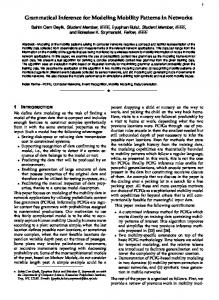
Figure 2. An example of pta.

The first task rpni∗ achieves is the construction of the pta (prefix tree acceptor ) of the words of E+ , that is the greatest trimmed dfa accepting only the words of E+ (see Figure 2). Its states are numbered following the hierarchical order over the prefixes of E+ . Then rpni∗ runs along these states following the ordering. Merging two states means to collapse them into a new one, whose number is the smallest of the two merged ones. With rpni, two states are mergeable if no negative example is contained in a final state. rpni∗ relaxes this constraint in order to authorize the presence of noisy words. A state is positive (or final) if it contains strictly more positive words (of E+ ) than negative ones (of E− ), and negative otherwise. A negative (resp. positive) word is misclassified if it is contained by a positive (resp. negative) state. Finally, a merging is statistically acceptable if the proportion of misclassified words in the whole dfa after the merging is not significantly higher than the proportion of misclassified words computed before the merging. This way to proceed allows to avoid overfitting phenomena.

A ←− pta(E+ ); for i = 1 to N − 1 do j ←− 0; continue ←− true; while (j < i) and continue do B ←− compute merging(A, i, j); C ←− compute final states(B, E+ , E− ); if statistically acceptable(C, E+ , E− ) then A ←− C; continue ←− false; j ←− j + 1; return(A);

Algorithm 2: Pseudo-code of rpni∗ . 4 b

3 a

b b

a 0

1

5

b

Figure 3. The effect of noisy data on the dfa.

In order to show the relevance of rpni∗ , let us consider that the noisy word bbbb is inserted in E− in the example already described in introduction. According to the target dfa (Figure 1), this word should be positive. Figure 3 shows the new profoundly modified dfa inferred by rpni, expressing well the fact that it is not immune to overfitting. Run on this problem, rpni∗ is able to infer the target dfa, handling optimally the noise. However, one hopes that misclassified examples are really noisy, that is the case for bbbb on this simple example. But due to its statistical nature, rpni∗ can statistically infer a bad merging. Although one can theoretically reduce this risk, it cannot be null, and can have dramatic effects on rpni∗ ’s performances. We aim here at collecting information about the confidence in the label of each example, and using it in a boosting procedure. Assuming that this information is given by an oracle, we would be able to detect which misclassified examples deserve to be learned or not. In other words, we would be able to separate the misclassified examples that must be subject to a weight increase, and those that deserve a weight drop. However, this requires the construction of a new optimal weighting scheme. That is the aim of the next section.

3. Boosting using a Confidence Oracle Let E be the set of |E| = m examples. Every x ∈ E has a label y(x) that can be positive (+1) or negative (−1). We assume that we have access to a confidence oracle, which gives to every example x a non-null real-

valued confidence q(x) ∈ [−1, 1], q(x) 6= 0. q(x) does not change throughout learning. A positive confidence means that x belongs to the class it is assigned to in E. A negative confidence means that we cannot be confident in its label. We partition E into the following sets: EN = {x ∈ E : q(x) < 0} and EN = E\EN . Since we cannot be confident in the labels of EN , we aim at minimizing by boosting the empirical error on EN , such that ∀T > 0, X [[y(x) 6= HT (x)]], (1) ε(EN , HT ) = (1/|EN |)

Comparing it with boosting’s second conP straint, (3) says that (w qyht )(x) = t+1 x∈EN P (w q)(x). Since ∀x ∈ E , q(x) < 0, the t+1 N x∈EN right member is strictly negative, which makes ht , the last hypothesis built, particularly bad on EN with a distribution depending on both wt+1 and q. These are clearly differences with classical boosting, which would yield an average (random) performance, on wt+1 alone and over E. The minimization of the information divergence under constraints (2) and (3) is obtained as the solution to (∀x ∈ E):

x∈EN

with [[π]] the indicator value in {0, 1} of the predicate PT π, and HT (x) = t=0 ct ht (x) the whole combined hypothesis (using the same notations as in Algorithm 1). Let Pm be the m-dimensional probability simplex, and u ∈ Pm the uniform vector. We assume a discrete probability vector wt ∈ Pm containing for each x ∈ E its weight at time t, with w0 = u (as in adaboost). We aim here at finding the new optimal update rule. It is known since Kivinen and Warmuth (1999) that standard boosting, as defined in Freund and Schapire (1997); Schapire and Singer (1999), is a particular case of the constrained optimization of a Bregman divergence. Let us recast this problem in our setting. The strategy is to repeatedly compute wt+1 from wt following the minimization of the information divergence, P 1.i(wt+1 , wt ) = x∈E i(wt+1 , wt )(x), with i(., .) the vector whose component for some x ∈ E is: ¶ µ wt+1 − wt+1 + wt (x). i(wt+1 , wt )(x) = wt+1 ln wt The information divergence is convex in wt+1 . One wishes to minimize 1.i(wt+1 , wt ) subject to two constraints. The first one is straightforward: it expresses the fact that wt+1 is a distribution (wt+1 ∈ Pm ): 1.wt+1 − 1 =

0.

(2)

In our case, this constraint remains the same. The second one integrates the loss function for each example in E. In classical boosting, it expresses that the last hypothesis found, ht , is in one sense the worst on the new distribution, Psince it performs on average like random guessing: x∈E (wt+1 yht )(x) = 0. This constraint, together with a so-called weak learning assumption (Kearns & Vazirani, 1994), ensures that the new hypothesis ht+1 built on wt+1 is significantly different from ht , thereby learning something ”new” over E. In our case, this constraint is a bit different: wt+1 .at ∀x ∈ EN : at (x) ∀x ∈ EN : at (x)

=

0,

= q(x)(yht )(x), = −q(x).

(3)

∂wt+1 i(wt+1 , wt )(x) ¤ + bt ∂wt+1 (1.wt+1 − 1) + ct ∂wt+1 (wt+1 .at ) (x) £

(4) = 0

with bt and ct Lagrange multipliers. Solving (4) for wt+1 brings ∀x ∈ E: ¶ µ wt+1 + bt 1 + ct at (x) = 0 ln wt ⇔ wt+1 (x) = wt (x) exp(−ct at (x)) / exp(bt ). Constraint (2) yields: X bt = ln wt (x) exp(−ct at (x)),

(5)

x∈E

The term inside the “ln” is the normalization coefficient for wt+1 : X Zt = wt (x) exp(−ct at (x)). (6) x∈E

We shall see hereafter that ct is in fact > 0 (Lemma 2). Since the oracle is confident in the label of any x ∈ EN (q(x) > 0), and since for any such example, wt+1 (x) = wt (x) exp(−ct q(x)(yht )(x))/Zt , it comes that the weight of any x ∈ EN increases in the next distribution iff it is misclassified by the current hypothesis ((yht )(x) = −1), and it decreases otherwise. On the other hand, the weight of all suspicious examples x ∈ EN (q(x) < 0) will ineluctably decrease: wt+1 (x) = wt (x) exp(ct q(x))/Zt . We will see in the next section that such an update rule improves rpni∗ ’s behavior. The last unknown, ct , is obtained from constraint (3) as the solution to: X (wt at )(x) exp(−ct at (x)) = 0. (7) x∈E

Notice that this is also stating (∂Zt /∂ct ) = 0. Since Zt is a convex function of ct , solving (4) ultimately returns to the problem of minimizing Zt . To see why solving (4) is so important, let us temporarily shift to the error committed by HT .

Lemma 1 ε(EN , HT ) ≤ (m/|EN |)

Q

t≤T

Lemma 2 The solution to (7) is unique and strictly positive, as it satisfies:

Zt .

Proof: Because ∀x ∈ EN , q(x) > 0, we have for any P such example [[HT (x) 6= y(x)]] ≤ exp(−q(x)y(x) t≤T ct ht (x)). On the other hand, wT +1 (x) = wT (x) exp(−q(x)y(x)cT hT (x))/ZT . Unraveling the update rule, EN : wT +1 (x) = P we get ∀x ∈ Q w0 (x) exp(−q(x)y(x) t≤T ct ht (x))/( t≤T Z Qt ), hence [[HT (x) 6= y(x)]] ≤ mwT +1 (x)( t≤T Zt ). Summing Q over all xP∈ EN , we get ε(EN , HT ) ≤ (m/|EN |)( t≤T Zt )( x∈E wT +1 (x)). Using the fact N P that x∈E wT +1 (x) ≤ 1, we get the Lemma. N

Since the term factoring the product of the normalization coefficients is constant given E and EN , Lemma 1 means that in order to drive down the error on EN to zero, we should concentrate on minimizing each Zt . This makes us kill two birds in one shot: solving (7) yields both the solution to (4), and (hopefully) the minimization of the error on EN according to Lemma 1. Let us concentrate on the solution to (7), under the assumption: ∀t ≥ 0, ∃γt > 0 a constant such that: X

x∈EN

(wt qyht )(x)

/

X

(wt q)(x) = γt .

(8)

x∈EN

Following boosting, we refer to (8) as a weak learning assumption (WLA), in particular since if ht were random, we would have γt = 0. In other words, (8) traduces the fact that ht must outperform random guessing by only a small amount for being considered as a weak hypothesis. Our WLA has two differences with classical boosting (Kearns & Vazirani, 1994). First, it is local: it puts emphasis on a subset of E. Second, it relies on a distribution which is not exactly wt , but a distribution wq,t ∈ Pm which is leveraged by q, as follows: ∀x ∈ E, wq,t (x) = |q(x)|wt (x)/Qt , with P Qt = x∈E |q(x)|wt (x) the normalization coefficient. Notice that ∀wt ∈ Pm , Qt 6= 0 because every example has q(.) P 6= 0. We extend this definition to that of Wq,t (E 0 ) = x∈E 0 wq,t (x) for all E 0 ⊆ E. To complete our discussion on constraint (3), define − + = {x ∈ EN : (yht )(x) = +1} and EN = {x ∈ EN ,t ,t EN : (yht )(x) = −1}. The WLA is equivalent to: − + ) − Wq,t (EN ) = γt Wq,t (EN ). Wq,t (EN ,t ,t

(9)

So we cannot choose ht+1 = ht under the WLA, since otherwise (3) would imply + − Wq,t+1 (EN ) − Wq,t+1 (EN ) < 0, while (9) would ,t ,t + − imply Wq,t+1 (EN ) − Wq,t+1 (EN ) > 0. Thus the ,t ,t WLA enforces ht+1 to learn something ”new”.

− − 1 − Wq,t (EN ) ) 1 − Wq,t (EN 1 1 ,t ,t ln ≤ c ≤ , ln t 2q 2q Wq,t (E − ) Wq,t (E − ) N ,t

N ,t

with q = minx∈E |q(x)| and q = maxx∈E |q(x)|. Proof: We define X (wt at )(x) exp(−cat (x)). g(c) =

(10)

x∈E

P g 0 (c) = − x∈E (wt a2t )(x) exp(−cat (x)) < 0. Thus, g(c) is strictly decreasing on R. Since limc→+∞ g(c) = −∞ (provided some x ∈ E has at (x) < 0) and limc→−∞ g(c) = +∞ (provided some x ∈ E has at (x) > 0), eq. (7) has a single solution. We have: g(0) Qt

− + ) − Wq,t (EN ) + Wq,t (EN ) = Wq,t (EN ,t ,t

= γt Wq,t (EN ) + Wq,t (EN ) = γt + (1 − γt )Wq,t (EN ).

(11)

We obtain g(0) > 0, which yields ct > 0 in eq. (7). Moreover, P g(ct ) =0= x∈E + ∪EN wq,t (x) exp (−ct |q(x)|) N ,t Qt P − x∈E − wq,t (x) exp (ct |q(x)|). N ,t

As q ≤ |q(x)| ≤ q for all x ∈ E, we get

− + ∪ EN )e−ct q − Wq,t (EN )ect q ≤ 0 and Wq,t (EN ,t ,t + − Wq,t (EN ∪ EN )e−ct q − Wq,t (EN )ect q ≥ 0. ,t ,t

Solving for ct yields the inequalities we claimed. − − ))/Wq,t (EN,t )) is soluThus ct = r ln((1 − Wq,t (EN ,t tion to eq. (7), for some r ∈ [1/2q, 1/2q]. This bound is tighter than the one of Schapire and Singer (1999) (for whom ct ∈ R), and yields a very-fast dichotomic approximation to ct . Suppose we want an approximation cˆt such that |ˆ ct − ct |/|ct | < ² for some 0 < ² ≤ 1. Then, it is is enough to make O(ln(q/q) + ln(1/²)) dichotomic rounds. It is very convenient, given that the computation of cˆt is repeated T times.

Lemma 3 ∀t ≥ 0, s à ¶ µ ¶2 ! µ qγt 2 1 qγt < exp − . Zt ≤ 1 − q 2 q

Proof: We have ∀x ∈ [−1, 1], ∀η ∈ R: exp(−ηx) ≤

1+x 1−x exp(−η) + exp(η), (12) 2 2

since function x 7→ exp(−ηx) is convex and the righthand side is the equation of the line crossing the two points (−1, exp(η)) and (1, exp(−η)). Plugging η = ct q and x = at (x)/q, ∀x ∈ E, yields exp(−ct at (x)) ≤ q + at (x) q − at (x) exp(−ct q) + exp(ct q). (13) 2q 2q Let us name `(x, ct ) the right-hand side of ineq. (13). We have X Zt ≤ inf wt (x)`(x, c). (14) c∈R

x∈E

The real c minimizing the right-hand side of (14) is P q + x∈E (wt at )(x) 1 P , ln c = 2q q − x∈E (wt at )(x) from which we get Zt

≤

s

1−

µ

g(0) q

¶2

,

(15)

with g(.) defined as in eq. (10). Using the fact that g(0) ≥ γt Qt (from eq. (11)), and Qt ≥ q, we obtain the statement of the Lemma. Provided q and q are constants (it shall be the case in our experiments), the maximal value of Zt is also a constant < 1 under the WLA, thus yielding the exponential convergence of ε(EN , HT ) towards 0.

4. An Oracle Simulation We describe in this section an empirical approach for simulating an oracle, which must satisfy at best the theoretical behavior previously mentioned. The main objective is to ensure that a positive confidence given by the oracle means that the example is (very probably) correctly labeled. We provide here a neighborhood-based strategy allowing to geometrically distinguish suspicious words from the others. 4.1. Neighborhood-based Confidence We think that the k nearest neighbor graph (kNN) (Cover & Hart, 1967) is suitable for treating such a problem. kNN’s classification rule assesses the class of an unknown example x by computing the majority

class among the k examples of E that are the closest to x. This method, beyond the fact that its limit error is bounded by twice the Bayesian error, is very tolerant to the presence of noisy data. Actually, an isolated outlier can only have a limited impact in the classification rule. The dual property, that we can deduce from the previous remark, is that a noisy data can be probably detected by analyzing its neighborhood. Let us define the margin function m(x) of an example x of class y(x), computable from a kNN graph: m(x) = (Ny(x) − Ny(x) )/(Ny(x) + Ny(x) ), where Ny(x) (resp. Ny(x) ) denotes the number of examples among x’s k nearest neighbors from the same class y(x) (resp. the opposite class y(x)). Hence an example with only neighbors from the opposite class (resp. from the same class) will receive −1 (resp. 1) as margin. Even if m(x) seems to assess in a way the confidence value q(x) used in the previous section, setting exactly q(x) = m(x) would not be judicious. Actually, the kNN classifier allows “only” to ensure that the limit error will be bounded by twice the Bayesian error, that is not in fact our main concern. We aim here at providing a relevant measure of confidence, ensuring that a positive q(x) means that x has a correct label in (100-²) percent of cases (with ² small). If m(x) is slightly higher than 0, this condition is far from being satisfied. To overcome this drawback, we fix a parameter β ∈ [0, 1[ and compute q(x) as follows: q(x) = (m(x) − β)/(1 − β) ∀ x such that β ≤ m(x) ≤ 1 (thus, q(x) > 0 iff m(x) > β); q(x) = (m(x) − β)/(1 + β) ∀ x such that −1 ≤ m(x) ≤ β. Roughly speaking, high confidences are only given to examples having a large majority of neighbors from the same class. While some examples are probably (weakly) relevant, i.e. having a margin just slightly higher than 0, they will receive a negative confidence. This choice will be useful in grammatical inference, where reducing the impact of relevant data is better than inferring a dfa from noisy words. 4.2. A Probability-Based Distance Function Before computing confidence values, we must use a relevant distance function between words. In this context, various distances have been studied, and the most popular one is probably the edit distance. However, we observed in preliminary experiments that we could obtain better results by using “data-oriented” distances, built after a transformation of the representation space. We decided to use bigram language models for describing words as vectors. Bigrams are a wellstructured knowledge representation that has proven useful in the recognition of textual documents. This

Table 1. Error rates obtained on 11 datasets with 5, 10, 15 and 20% of noise. Dataset Agaricus TicTacToe USF WF Base1 Base2 Base3 Base4 Base5 Base6 Base7 Average

size 5644 809 1871 1887 2540 1505 1532 2969 2179 2004 10000 2994.5

knn 0.0% 9.2% 16.5% 16.4% 24.8% 9.6% 10.4% 0.5% 0.9% 17.7% 23.0% 11.7%

rpni 7.2% 39.5% 33.6% 29.3% 46.4% 48.9% 43.9% 39.7% 36.7% 42.9% 46.1% 37.7 %

Agaricus TicTacToe USF WF Base1 Base2 Base3 Base4 Base5 Base6 Base7 Average

5644 809 1871 1887 2540 1505 1532 2969 2179 2004 10000 2994.5

1.0% 15.4% 20.5% 20.4% 28.2% 12.9% 12.7% 1.5% 2.0% 24.9% 27.1% 15.1%

14.0% 44.0% 34.9% 32.5% 47.0% 39.8% 47.0% 44.2% 44.5% 50.6% 48.0% 40.6%

5% rpni∗ 7.2% 34.5% 31.2% 25.3% 41.5% 21.9% 27.0% 2.0% 36.7% 7.0% 39.7% 24.9% 15% 10.0% 40.7% 32.0% 36.2% 42.9% 39.8% 39.4% 16.0% 43.8% 42.9% 40.7% 34.9%

boost 4.3% 28.3% 26.1% 21.4% 41.1% 19.9% 26.7% 10.0% 22.2% 13.0% 37.2% 22.7%

perf 0.0% 4.9% 26.4% 20.6% 35.6% 14.3% 13.0% 0.0% 19.2% 2.0% 39.7% 16.0%

knn 0.0% 16.0% 16.8% 19.3% 27.8% 9.6% 11.0% 1.0% 1.3% 21.6% 25.1% 13.6%

rpni 14.0% 41.9% 35.7% 29.8% 52.1% 39.2% 39.0% 45.7% 45.9% 45.9% 49.4% 39.9%

6.1% 40.7% 27.7% 24.6% 42.3% 37.5% 35.5% 26.9% 31.4% 33.1% 43.2% 31.7%

0.0% 9.8% 27.7% 24.6% 38.5% 10.6% 14.9% 0.0% 15.1% 1.7% 40.7% 16.7%

2.0% 17.9% 23.7% 22.2% 31.1% 16.9% 18.5% 3.3% 2.2% 28.9% 29.2% 17.8%

23.2% 40.1% 48.8% 35.4% 51.2% 46.8% 49.5% 43.4% 41.0% 46.6% 48.0% 43.1%

makes it possible to apply geometric, and other mathematical techniques, which are well defined for vectors, but not for words in general. The probability of a letter of a word depends only on the identity of the preceding letter. QnGiven a word with n letters x = l1 l2 l3 . . . ln , p(x) = i=1 p(li /li−1 ). To make p(l1 /l0 ) meaningful, a distinguished token (for beginning of the word) is added and we take l0 as . Here, we aim at computing an euclidean distance from a twodimension numerical representation of words. Let us define P+ (x) and P− (x), Pb (x) denoting the probability of x relatively to the subset Eb . To allow comparisons between words of different lengths, we normalized each probability p using the geometric mean, as follows: Pb0 (x) = n+1 Pb (x). Given P+0 (x) and P−0 (x), we can now (i) see x as a point in an euclidean space with coordinates P+0 (x) and P−0 (x), (ii) compute the euclidean distance, and (iii) so build the kNN graph.

5. Experiments and Results The motivation of our experiments was not only to validate our theoretical results but also to assess the performances of the kNN graph as a good candidate for simulating an oracle. To achieve these tasks, we used three types of datasets. The first one concerns well known benchmarks of the uci repository: agaricus and TicTacToe. The second represents real-world datasets: a first one (USF) comes from the US Social Security Administration and takes the census of the first thousand first names the more frequently given in

10% rpni∗ 10.0% 40.7% 33.0% 31.2% 44.8% 13.6% 39.0% 29.2% 18.6% 42.9% 42.7% 31.4 % 20% 18.2% 40.1% 32.2% 32.0% 45.7% 46.8% 49.5% 35.0% 39.4% 41.9% 44.3% 38.6%

boost 6.9% 34.5% 31.2% 22.7% 43.7% 30.5% 12.7% 23.4% 25.0% 25.6% 43.7% 27.3%

perf 0.0% 10.5% 31.7% 26.1% 36.2% 12.3% 12.7% 0.0% 16.2% 1.2% 39.4% 16.9%

11.9% 38.8% 30.6% 31.7% 45.2% 45.1% 41.6% 30.4% 34.6% 39.2% 41.8% 35.5%

0.0% 11.7% 28.8% 22.7% 35.2% 12.6% 20.5% 0.0% 9.4% 1.0% 40.5% 16.6%

the USA in 2002; a second one (WF) contains all the worldwide first names that begin with the letter “a”. For both of them, the concept to learn is the gender of the individuals. The last type of datasets concerns artificial ones. We generated 7 synthetic databases (Base1,. . .,Base7) made of random words with variable length and labeled according if they contain a priori fixed patterns or not. To test our method on a large dataset, Base7 contains 10000 words. For all the 11 databases, we introduced noise, by switching the class of a given percentage of words and we assessed the error rate using a noise-free test set. Table 1 compares rpni, rpni∗ and our boosting approach (boost) after 200 iterations for the different levels of noise. Two other columns have been added in this Table. The first one (knn) describes the performances of the kNN graph as a single classifier (i.e. without boosting, without dfa). The interest of these results is not only to show how well a kNN graph simulates the oracle, but also to estimate the gain obtainable using it in a boosting procedure. The second column (perf) presents the results obtained from a perfect oracle, i.e. one that always knows if a data is noisy or not. The goal of this column is to establish the optimal (but unobtainable) error rate for each database. This experimental study was achieved with 5, 10, 15 and 20% of noise. We tried different values of k (for the kNN graph) and kept the optimal value (assessed by cross-validation) for each database. The following remarks can be made. First of all, the

excellent results obtained in the column kNN justify the use of the kNN graph as a simulated oracle. While rpni∗ constituted a first efficient solution for improving rpni (32.5% versus 40.3% on average on all the noise levels), our new oracle-based boosting procedure results in a dramatic improvement of the performances. Actually, the additional information provided by the kNN graph, and used in our boosting method, permits to significantly decrease rpni∗ ’s error rate (29.3% versus 32.5% on average). This difference is statistically significant using a Student pairedt test. Another interesting remark is that the use of our simulated oracle results in final hypotheses whose performances are not so far, after 200 iterations, from the ones issued from the perfect oracle (29.3% versus 16.5% on average). Finally, note that the previously described behaviors remain almost the same even with the increase of the noise level.

References

In order to show the exponential convergence of the generalization error all along the iterations, Figure 4 describes the behavior of the algorithm on 4 characteristic databases (for 5% of noise). It brings to the fore the rapid effect of boosting on the performances (often before the 20th iteration).

Freund, Y., & Schapire, R. E. (1996). Experiments with a new boosting algorithms. Thirteenth Int. Conf. on Machine Learning (pp. 148–156).

0.5 Agaricus WF USF Base7

0.45

Blum, A., & Mitchell, T. (1998). Combining labeled and unlabeled data with co-training. 12th Int. Conf. on Computational Learning Theory (pp. 92–100). Cover, T., & Hart, P. (1967). Nearest neighbor pattern classification. IEEE Trans. on Information Theory, 13, 21–27. de la Higuera, C. (2004). A bibliographic survey on grammatical inference. Pattern Recognition. To appear. Domingo, C., & Watanabe, O. (2000). Madaboost: a modification of adaboost. Third Annual Conf. on Computational Learning Theory (pp. 180–189). Freund, Y. (2001). An adaptive version of the boost by majority algorithm. Machine Learning, 43, 293–318.

Freund, Y., & Schapire, R. E. (1997). A DecisionTheoretic generalization of on-line learning and an application to Boosting. Journal of Computer and System Sciences, 55, 119–139. Friedman, J., Hastie, T., & Tibshirani, R. (1998). Additive logistic regression: a statistical view of boosting (Technical Report).

0.4 0.35

Kearns, M. J., & Vazirani, U. V. (1994). An Introduction to Computational Learning Theory. M.I.T. Press.

Error

0.3 0.25 0.2

Kivinen, J., & Warmuth, M. (1999). Boosting as entropy projection. Twelfth Int. Conf. on Computational Learning Theory (pp. 134–144).

0.15 0.1 0.05 0 0

50

100 T

150

200

Figure 4. Generalization error in function of iterations.

6. Conclusion We introduced a new boosting scheme that allowed to improve the performances of a grammatical inference algorithm in the presence of noisy data. As far as we know, our approach on using a real-valued confidence oracle for boosting is new, even outside grammatical inference, and deserves to be applied with other weak learners. Moreover, we proposed a heuristic based on neighborhoods for efficiently building this oracle. The study of other types of oracles, such as hidden Markov models, also deserves further investigations.

Lang, K., Pearlmutter, B., & Price, R. (1998). Results of the abbadingo one dfa learning competition. Fourth Int. Colloquium on Grammatical Inference (pp. 1–12). Oncina, J., & Garc´ıa, P. (1992). Inferring regular languages in polynomial update time, vol. 1 of Machine Perception and Artificial Intelligence, 49–61. World Scientific. Schapire, R. E., & Singer, Y. (1999). Improved boosting algorithms using confidence-rated predictions. Machine Learning, 37, 297–336. Sebban, M., & Janodet, J. (2003). On state merging in grammatical: a statistical approach for dealing with noisy data. Twentieth Int. Conf. on Machine Learning (pp. 688–695).