We also show that such technique has a low computational overhead time. 1. Introduction ... traffic. Therefore, due to the huge amount of data produced by flow measurement, it is ..... Bootstrap estimate of the variance of Y is approximately ns/2.
Bootstrap-Based Estimation of Flow-Level Network Traffic Statistics Stenio Fernandes, Tatiene Correia, Carlos Kamienski, Djamel Sadok Universidade Federal de Pernambuco, Centro de Informática CP 7851, Recife-PE, 50732-970 {sflf, tatiene, cak, jamel} @cin.ufpe.br
Abstract: Network traffic measurement and analysis have been playing an important role in traffic engineering, and network planning. Most recent research papers in this field have been focusing to passive flow measurement since collecting packet-level data in high-speed links is prohibitively expensive. Although there are techniques for handling flow statistics in modern routers, transmitting and storing flow-level information still imposes a significant burden on the network management operation. In this paper, we advocate that only a small portion of the flow records need to be preserved for further processing. We propose the use of the Bootstrap resampling technique for deriving properties from a previously pre-processed sampled set of flows. Our results show that only 10% or less of the original sampled statistics is necessary in order for Bootstrap to reconstruct the characteristics of the original raw flow records. We also show that such technique has a low computational overhead time.
1. Introduction Monitoring backbone network traffic is a mandatory task to manage today's complex Internet Service Providers (ISP) infrastructure. Particularly, computer networking researchers have been made great efforts to make the systemic nature of the Internet more comprehensible, based on passive and active measurements. Hence, network measurements are essential for appraising systems performance, identifying and locating problems in high-speed links [11]. Further, measurement information has been widely used by ISPs for short-term monitoring (e.g., detecting denial-of-service attacks [18]), long-term traffic engineering and provisioning (e.g., forecasting link upgrade [10]), and accounting (e.g., establishing usage-based pricing [14]). In order to obtain such information, today's routers offer tools such as NetFlow that provides flow level information about traffic. As new applications arise in the Internet (e.g., peer-to-peer systems) network operators need more accurate information related to the workload of their network, such as relative volumes of traffic using different ports and protocols, number and duration of flows traversing their routers, traffic matrices etc. However, the main obstacle with the flow measurement approach is its lack of scalability with link speed. For instance, some recent measurements [15] show that the number of flows in an unsampled raw NetFlow trace collected in an aggregated link during 1 day in September 2002 reaches 229,448,460 records. As link speeds and number of flows increase, holding a counter for each flow may be too expensive or slow [4]. Therefore, packet-sampling techniques are progressively being used in routers to export statistics of a fraction of the network traffic [13]. Although packet sampling is a widespread technique, one difficulty that arises is how to deal with
partial measurements. It is imperative to recover statistics of the original traffic from such partial sampled data through some reliable procedure. Network Managers and Engineers usually support their decisions based on characteristics of the full network traffic. Therefore, due to the huge amount of data produced by flow measurement, it is necessary for routers to control the usage of processing resources, network capacity used to transfer data to collectors, and processing and storage costs at the collectors. Likewise, collecting IP packet headers will give rise to an immense amount of data. This could cause ever increasing demands and costs, e.g., on computational resources at the measurement point and systems for data storage and analysis. This paper analyses the possibility to derive properties of the original traffic stream from the packet sampled flow statistics, using a well-known resampling technique called Bootstrap [1][3]. We extend the analysis presented previously in [20], to evaluate the processing overhead time of such resampling technique. We consider such methodology very appealing and we think it could be applied to a number of circumstances. For instance, Bootstrap estimates could be accurately inferred from light and heavy tailed distribution functions. This opens the doors to the possibility of performing a smooth sampling technique and also achieving a high level of accuracy of the Bootstrap estimates related to the original traffic characteristics. Therefore, considering a variety of network traffic profiles, it seemed promising to look at alternative procedures to reduce the volume of the sampled network traffic data. In order to provide useful examples of the applicability of the Bootstrap technique, we analyzed packet and flow-level traces. Our results show that after a after a small amount of pre-processing in the raw data and extracting some metrics from traces (e.g., flow size and duration), it is necessary to store or transmit only 10% of the original sampled statistics, in order for Bootstrap to precisely reconstruct its main properties. Using Bootstrap analysis to characterize the statistical properties of data has lately become a useful and widespread tool in a number of research fields[9][7][19][8][5]. For instance, Buvat and Riddel [9] proposed the nonparametric bootstrap method to characterize the statistical properties of computed tomography images. White and Racine [7] investigated the use of bootstrap methods for inference using artificial neural networks applied to predictive accuracy in foreign exchange rates. Recently, Lei and Smith [19] presented some results on an empirical analysis of the reliability of nonparametric bootstrap method in assessing the accuracy of sample statistics in the context of software metrics. Liu et al. [5] proposed the use of Bootstrap method in order to predict fine time-scale behavior of network traffic from coarse timescale aggregate measurements. Therefore, as far as we know, research studies related to applying bootstrap in the network traffic management field have not been well explored. The paper is organized as follows. Section 2 presents related work. Section 3 develops the basic theory of the Bootstrap methodology and describes its application in common network traffic properties. The next section (Section 4) shows our validation results of the Bootstrap method based on real network traffic. We use both NetFlow and NLANR data. Finally we draw some conclusions and present suggestions for future work in Section 5.
2. Related Work There are a number of recent research papers related to the problem of packet sampling and recovering statistics of the original traffic from sampled data. Some of them focus only on the problem of sampling inside routers whereas others are more interested in resource utilization and analysis in a measurement infrastructure [14][16][15][4][12][2]. Sampling methods have been advocated to reduce the volume of sample data on the measurement infrastructure. The goal is to estimate some traffic properties (e.g., the packet size distribution) from the sampled packets. In order to reach a better performance at lower effort, a number of sampling strategies have been studied. It is possible to deterministically take one in every N packet (regular sampling), take on average one in N packets (simple random sampling) or take one packet in every bucket of size N (stratified random sampling). However, Duffield [15] showed that those sampling techniques are naïve, because they cause the loss of information of short traffic flows. Estan and Varghese [4] proposed two scalable algorithms for identifying large flows named “sample and hold” and multistage filters. They found out such algorithms to be highly efficient because they would take a constant number of memory references per packet and use a small amount of memory. The main motivation of their work is that a few heavy and long-lived flows dominate the current Internet traffic. They addressed the issue of identifying these heavy flows without keeping track of millions of small flows. The proposed algorithms presented a clear advantage against NetFlow’s sampling technique, since they provide exact values for long-lived large flows and lower bounds on traffic, avoid resource intensive collection of large NetFlow logs, and identify large flows very fast. However, this preference on recording longer flows could lead to some bias in the total traffic volume. Moreover, it could not approximate to the empirical distribution function of the flow lengths. For this situation, we think that Bootstrap could be used as a complementary procedure to handle short flows with little resource consumption in routers. In this case, Bootstrap would correct the bias and recover the missing information related to the small flows. In [15] Duffield et al. presented approaches to accurately infer the distributions of flow lengths in the original Internet traffic based on the flow statistics formed from sampled packet streams. Their main contribution is inferring flow numbers and lengths of the original traffic that escaped thinning process completely. They reasoned that as only sampled flow statistics are available (particularly in high-speed routers) some statistical inference is needed to fully determine the flow characteristics of the original unsampled traffic. Firstly, their work accurately predicted the distributions of flow lengths shorter than a determined threshold N. They used Maximum Likelihood Estimation (MLE) to estimate the full distribution of packet and byte lengths. MLE is consistent because it becomes unbiased as the sample size increases. Likewise, in [14] Duffield et al. replaced uniform sampling with size dependent sampling, in which an object of size X is selected with some size dependent probability p. Hence, this approach allows controlling the rate at which samples are produced. The main motivation here was to perform accurate usage-sensitive billing from sampled flow statistics. They showed that is not possible for a router to keep counters on all traffic flows, either because they are too numerous, or because the set of flows is very dynamic. Similarly, in [16] Duffield et al. determined resource usage, for both
construction and transmission of flow statistics, and showed how it depends on the flow’s characteristics. Afterward they recovered some detailed statistical properties of the original packet stream from the packet sampled flow statistics (e.g., the number and lengths of flows). Traffic Analysis Platform (TAP) was proposed in [12] to support detailed information on network resource usage, such as the relative volumes of traffic using different protocols, traffic matrices or the aggregate statistics of packet and byte volumes and durations of user sessions. TAP relies on a distributed infrastructure and on the use of sampling and aggregation at different measurement locations. Three entities form the TAP architecture, namely Routers, Collectors/Aggregators and a Data Warehouse. Router’s function is to accumulate NetFlow records on the traffic passing through, which are exported to a local Collector. Collector/Aggregator’s functions are to receive raw NetFlow records from the routers, aggregate them and create several higherlevel records. Then, these aggregates are sent to a central Data Warehouse, which stores the aggregate data. A non-uniform sampling presented in [14] of the completed NetFlow records is applied at the Collectors for controlling resource usage, based on the empirical fact that flow sizes have a heavy tailed distribution. One should notice that cascading down sampling reduces the information that flows through TAP. Therefore, it is highly necessary to compensate such burden in order to get an unbiased estimate of the properties in the original traffic. As we will present in Section III (Bootstrap), Bootstrap is highly efficient in handling light and heavy-tailed probability distribution functions. Thus, such technique could be applied to recover missing information traversing its elements in TAP. Furthermore, Bootstrap procedures could be added to the Collector or to the Data Warehouse in order to allow lessening the data volume traveling through the network. In other words, one should also rely on the power of Bootstrap to reduce storage volumes while maintaining the ability to recover statistic properties of the original data from the sample.
3. Bootstrap Method In this section we discuss techniques, which are applicable to a single, homogeneous sample of data, denoted by y1 ,..., y n . The Bootstrap method follows the plug-in principle, which states that given a parameter of interest depending on CDF F, estimate it by replacing F by its empirical counterpart obtained from the observed data. This is referred to as the Bootstrap Estimate of that parameter. Let the sample data be outcomes of Independent and Identically Distributed (IID) random variables Y1 ,..., Yn whose Probability Density Function (PDF) and Cumulative Distribution Function (CDF) we shall denote by f and F , respectively. The sample is used to make inferences about a population characteristic, generically denoted by θ , using a statistic T whose value is t . We assume for the moment that the choice of T has been made and that it is an estimate for θ , which we take to be a scalar. There are two types of Bootstrap techniques: parametric and nonparametric procedures. When we have a particular probability distribution model, with parameters that fully determine f , such a model is termed parametric and statistical methods based on this model are parametric methods. When no such probability distribution model is specified, the statistical analysis is nonparametric, and it relies only on the fact that the
random variables Y j are Independent and Identically Distributed. Even if there is a plausible parametric model, a nonparametric analysis can still be useful to assess the robustness of conclusions drawn from a parametric analysis [12]. An important role is played in nonparametric analysis by the empirical distribution, which puts equal probabilities n −1 at each sample value y j . The corresponding estimate of F is the Empirical Distribution Function (EDF) Fˆ . When there are repeated values in the sample, as would often occur with discrete data, the EDF assigns probabilities proportional to the sample frequencies at each distinct observed value y . Several statistics could be derived from Fˆ . In general, the statistic of interest t is a symmetric function of y1 ,..., yn and it is not affected by reordering the data, depending only on Fˆ . This fact is frequently expressed simply as y = t (Fˆ ) where t (.) is a statistical function. Such statistical function is of vital importance in the nonparametric case since it also defines the parameter of interest θ through θ = t (F ) . It corresponds to the qualitative idea that θ is a characteristic of the population described by F . The relationship between the estimate t and Fˆ could usually be expressed as t = t (Fˆ ) corresponding to the relation θ = t ( F ) between the characteristic of the interest and the underlying distribution. The statistical function t (.) defines both the parameter and its estimate, but we shall use t (.) to represent the function, and t to represent the estimate of θ based on the observed data y1 ,..., y n . Suppose that we have no parametric model, but that it is reasonable to assume Y1 ,..., Yn are IID according to an unknown distribution function F . We use the EDF Fˆ to estimate the unknown CDF F . We must use Fˆ just as we would do in a parametric model. In the case of the sample mean, exact moments under sampling from the EDF are easily found. For example,
E * (Y * ) =
n
1 y j = y and j =1 n
similarly var * (Y * ) =
{
}
1 * * E Y − E (Y * ) n
2
=
n
1 ( y j − y) 2 n j =1
Applying simulation with the EDF is very straightforward. Since the EDF puts equal probabilities on the original data values y1 ,..., y n each Y * is independently *
*
sampled at random from those data values. Therefore the simulated sample Y1 ,..., Yn is a random sample taken with replacement from the data. This simplicity is specific to the case of a homogeneous sample, but many extensions are straightforward. This resampling procedure is called the Nonparametric Bootstrap. Figure 1 is a schematic diagram of the bootstrap method as it applies to onesample problems [3]. The real world is on the left frame, where an unknown distribution F has generated the observed data y = ( y1 , y 2 , y n ) by random sampling.
We have calculated a statistic of interest from y , θˆ = s ( y ) , and wish to know something about θˆ' s statistical behavior (e.g., its standard error se F (θˆ) ). In the Bootstrap world (right frame), the empirical distribution gives bootstrap samples y * = ( y1* , y 2* , , y n* ) by random sampling, from which we calculate bootstrap replications of the statistic of interest, θˆ * = s ( y * ) . The main advantage of the bootstrap world is that one could calculate as many replications of θˆ * as one wish or at least as many as one can afford. REAL WORLD Unknown Observed Probability Random Distribution Sample
BOOTSTRAP WORLD Empirical Distribution
F → y = ( y1, y2 ,..., yn )
Bootstrap Sample
Fˆ → y * = ( y1* , y2* ,..., yn* )
↓ θˆ = s ( y )
↓ θˆ* = s ( y * )
Statistic of interest
Bootstrap Replication
Figure 1 - A schematic diagram of the bootstrap: one-sample problem.
In general, nonparametric Bootstrap will not work for serially dependent data. This can be illustrated quite easily where the set y1 , , y n form one realization of a correlated time series. For instance, consider the sample mean y and suppose that the
data come from a stationary series {Y j } whose marginal variance is σ 2 = var(Y j ) and whose autocorrelations are ρ h = corr (Y j , Y j + h ) for h = 1,2,
. The nonparametric
Bootstrap estimate of the variance of Y is approximately s 2 / n and for large n this will approach σ 2 / n . However the actual variance of Y is Var (Y ) =
σ2 n
(1 −
h n
)ρh .
The sum here would often differ considerably from the unity. Therefore the Bootstrap estimate of variance would be incorrect. The essence of the problem is that simple Bootstrap sampling imposes mutual independence on the Y j effectively assuming their joint CDF is F ( y1 ) × ... × F ( yn ) and thus sampling from its estimate * * Fˆ ( y1 ) × ... × Fˆ ( y n ) . This is a pitfall of the use of Bootstrap for dependent data. The difficulty is that there is no obvious way to estimate a general joint density for Y1 , , Yn given one realization. We present now two examples to reveal the power of the Bootstrap method. We utilized two dataset of length 10,000. The first (‘dataset 1’) was generated from a Normal PDF with mean zero and variance one. The second dataset (‘dataset 2’) was generated from a Weibull PDF with scale parameter 1.0 and shape parameter 1.5, which
corresponds to a probability model with mean 0.89 and variance 0.37. Later on, these two datasets were deterministically sampled, drawing 1 to N samples (N = 1000, 100, 10). The resulting sampled data will have sample lengths of size n = 10, 100 and 1000. We evaluated some metrics (mean and variance) for both sampled unsampled data. Moreover, we also exhibit the Quantile-Plot. Table 1 - Descriptive measurements (Mean) for ‘dataset 1’ and ‘dataset 2’. n = 10, 100, 1000 and nb = 500, 1000 .
Dataset 1 # of Sample Bootstrap Length Mean Bias Replicas 500
1000
Dataset 2 Mean
Bias
10
-0.24
-0.25
1.03
0.14
100
-0.14
-0.15
1.02
0.13
1000
0.02
0.01
0.94
0.05
10
-0.25
-0.26
0.95
0.06
100
-0.06
-0.07
1.01
0.12
1000
-0.03
-0.04
0.91
0.02
Table 2 - Descriptive measurements (Variance) for ‘dataset 2’ and ‘dataset 1’. n = 10,100,1000 and nb = 500,1000 . # of Bootstrap Replicas
500
1000
Dataset 1
Dataset 2
Sample Length
Variance
Bias
10
0.74
-0.27
0.32
-0.05
100
1.22
0.21
0.47
0.10
1000
1.07
0.06
0.40
0.03
10
1.64
0.63
0.39
0.02
100
1.17
0.16
0.46
0.09
1000
1.05
0.04
0.39
0.02
Variance Bias
Table 1 and Table 2 present the mean, bias and variance for the three sample data ( n = 10,100,1000 ) considering the number of Bootstrap replications ( nb ) as 500 and 1000. Our first impression for the results is particularly obvious. First, as the sample length grows the mean and the variance become more accurate. For instance, considering nb = 500, ‘dataset 1’ and n = 100, the mean of dataset is –0.14 with a bias equal to –0.15 whereas for n = 1000 such mean achieve 0.02, but with a bias equal only to 0.01. Second, with an overall observation on the bias, one should notice that an increase in the sample length implies in the decrease of this metric for both two dataset (‘dataset 1’ and ‘dataset 2’). For instance, considering nb = 500 and n = 100, the bias for the variance (dataset 2) is 0.10 whereas increasing sample length to n = 1000 , such bias reach 0.03. Analyzing the number of Bootstrap replications, we should depict several important conclusions. We notice that as nb increases the results get better. For instance, considering n = 100 and nb = 500 in Table 2, for ‘dataset 1’ the bias of the
4
variance is 0.21 and increasing the number of bootstrap replications twice, such bias decreases to 0.16. It is important to emphasize when the sample length is as low as 0.1% the methodology could not be valuable for the determination of the statistics properties of the original data. The conclusion that can be made from this experience is that, indeed, experiments using the bootstrap method should be carefully undertaken. Observing the variance and bias, one can control the degree of accuracy for any datasets.
1 -2
-1
0
quantile
2
3
Original n = 10 n = 100 n = 1000
0
20
40
60
80
100
Index
Figure 2 – Quantile-Plot: ‘dataset 1’
Figure 2 and Figure 3 present the Quantile-Plots from the ‘dataset 1’ and ‘dataset 2’, respectively (nb= 500). One should notice that even considering the length of the sampled data as low as 1% of the original data size, the technique could precisely mimic the original quartiles for both distribution, Normal and Weibull.
4 2 0
1
quantile
3
Original n = 10 n = 100 n = 1000
0
20
40
60
80
100
Index
Figure 3 - Quantile-Plot – ‘dataset 2’
We repeated the simulation considering several PDF typically utilized in the network traffic-modeling field (e.g., Pareto, Lognormal, Exponential etc.). In these circumstances, Bootstrap generated estimates with comparable accuracy. However, we will not present them here due to lack of space. Furthermore, if we sample 1 in each 10 realization from the original data (i.e., 10% of the original data size) the resulting Quantile-Plot is indistinguishable.
4. Experimental Application and Results The previous section presented a theoretical examination for the Bootstrap methodology for two different classes of data (Normal and Weibull PDF). In this section we present a numerical evaluation of the Bootstrap technique tackling some flow level statistics. Our data for the experiments were comprised of flow and packet level traces. The passive measurements (raw data) used to illustrate the Bootstrap Methodology came from a large ISP (NetFlow records). We pre-processed such traces (flow level) in order to get some metrics, namely the flow lengths and sizes. Additionally, we analyzed real data from the interfaces BWY – (Columbia University at Broadway), COS (Colorado State University) and TXS (Texas universities GigaPoP at Rice University) available at the NLANR website. We transformed the packet-level traces into the same metrics (flow length and size). Hence, results presented in this section consider each register in the datasets as flow duration (in seconds) or volume (in bytes). We achieved similar results for all packet-level traces and also for the flow-level ones. Therefore, in the following paragraphs, we chose to show only the results for the COS trace. Table 3 and Table 4 present the first and second-order statistics and their respective biases for three sample lengths considered (n = 15, 145, 1447, which correspond to 0.1%, 1% and 10% of the original trace, respectively). These sample lengths are the result of deterministic sampling performed in the pre-processed traces. The original sample dataset comprised approximately 15000 individual (flow-level
metrics) records. We also kept the number bootstrap replications (500 and 1000) for both ‘duration’ and ‘volume’ datasets. Table 3 - Descriptive measurements for the ‘time’ dataset; n = 15, 145, 1447 and nb = 500, 1000 . Original Mean (for Duration=35.06s; for Volume=0.14MBytes) # of Bootstrap Replicas
500
1000
Sample Length
Per-flow Duration (s)
Per-flow Volume (MBytes)
Mean
Bias
Mean
Bias
15
28.74
-6.32
0.01
-0.13
145
36.11
1.05
0.20
0.06
1447
35.23
0.16
0.15
0.01
15
29.99
-5.07
0.01
-0.13
145
36.17
1.11
0.22
0.07
1447
35.24
0.18
0.14
0.00
Table 4 - Descriptive measurements for ‘volume’ dataset; n = 15, 145, 1447 and nb = 500,1000 . Original Variance (for Duration =1.23e3; for Volume=2.23e12) # of Sample Bootstrap Length Replicas
500
1000
Per-flow Duration
Per-flow Volume Bias
Variance (x1e3)
Bias
Variance (x1e10)
(x1e10)
15
1.17
-614
1.73
-223
145
1.23
-4.17
167
-56.3
1447
1.23
2.35
131
-92.7
15
1.22
-17.1
0.0816
-223
145
1.22
-6.42
173
-49.9
1447
1.23
2.01
132
-91.0
In our experiments, we observed similar behavior to the simulation of section 2. Recall that the mean value for per-flow metrics presented in Table 3 refers to the average of flow duration and sizes. We could draw several conclusions from the results. First, if we focus on bias, we could state that increasing the sample length implies in diminishing the value of this metric for both datasets ‘duration’ and ‘volume’. For instance, considering nb = 1000 and n = 145, the bias is 1.11. If we increase the sample length to n = 1447, then the bias decreases to only 0.18. Second, as far as bootstrap replications are concerned, we observed that as nb increases from 500 to 1000, the results get better in most cases. For instance, for nb = 500 and n = 15, the bias for the variance is –614. Increasing twice the number of bootstrap replications, it reaches only 2.35, as shown in Table 4.
Original n = 15 n = 145 n = 1447
Figure 4 - Empirical Cumulative Distribution Function - ‘duration’ (in seconds).
Figure 4 presents the ECDF from the ‘duration’ dataset (in seconds). We set the number of Bootstrap replications (nb) to 500. One should observe that even with the length of the sampled data as low as 1% of the original data size, the Bootstrap technique could precisely mimic the original raw pre-processed data. Furthermore, if we gather records through 1 in 10 sampling from the original data (i.e., 10% of the original data size) the resulting ECDF remains indistinguishable. Figure 5 presents the ECDF for the per-flow volume dataset. The number of Bootstrap replications (nb) was set to 500. In the same way, the Bootstrap technique could accurately imitate the original preprocessed data with only 10% of the records.
Original n = 15 n = 145 n = 1447
Figure 5 - Empirical Cumulative Distribution Function – Volume (in Mbytes).
Figure 6 shows the results of the processing times evaluation. First, we generated a dataset with 100.000 samples from a Weibull PDF. Second, we reduced such dataset to 0.1%, 1% and 10% (Na = 100, 1000, and 10.000 respectively) of the original using uniform sampling. After that, we applied the bootstrap method varying the number of replicas as indicated in the axis X (Nb = 10, 50, 100, 200, 300, 500, and 1000), and calculated the mean processing times for a number of simulations. Clearly, as the number of replicas increases, the execution time of the processing time increases. For a small size sub-sampled set of data (i.e., 0.1% and 1% of the original dataset), the processing time remains stable with a slight increase. In such case, the computational time of the bootstrap technique is flat until 300 replicas and then starts to increase. However, for the biggest sub-sampled set of data (i.e., 10% of the original dataset) the processing time increases in an exponential manner. From this result, one can observe that there is a clear tradeoff between the number of replicas and the accuracy of the technique. Using the bootstrap method requires that experimenters should choose the number of replicas and the uniform sampling rate carefully. However, despite the exponential increase for large datasets, it is worth emphasizing that the processing time remains in a suitable level (below 5 seconds), using a standard computer configuration (2GHz processor with 256MB RAM) and a free software environment for statistical computing and graphics, named R [21]. Processing Overhead
Time (s)
5.0 4.5
Na - 100
4.0
Na - 1000
3.5
Na - 10000
3.0 2.5 2.0 1.5 1.0 0.5 0.0 10
50
100
200
300
500
1000
Number of Bootstrap Replicas
Figure 6 - Processing Time Evaluation
5. Concluding Remarks Motivated by the concerns of network operators in large ISP backbones that point out to an ever increasing huge amount of data produced by the passive measurement infrastructure, this paper undertake the problem of reducing such data volume without missing crucial statistical properties. We relied on the Nonparametric Bootstrap technique, which is a resampling procedure. We verified by simulation the Bootstrap performs well with a variety of probability functions. Due to its flexibility, we propose Bootstrap to be used as a technique to reduce data volume either in routers or in a post-processing element (such as the Aggregator in TAP). In practice, any effort to gather flow statistics involves classifying individual
packets into flows. For flow-level sampling, all packets have to be put into flows before they can be discarded. This is an apparent pitfall of using Bootstrap in routers as it could probably involve more computation and memory. However, as indicated in [13], this may not be a weakness if new flow classification techniques, such as Bloom filters [2], can be applied as an alternative. Hence deploying Bootstrap in a post-processing element is a viable solution to support reduction in data volume. Applying the methodology in real network traffic measurements, this paper showed that one could use Bootstrap to infer some general characteristics of the network traffic distribution. In order to provide useful examples, we analyzed packet and flowlevel traces. This paper points out that after executing a short pre-processing in the raw data and extracting some metrics from traces (e.g., flow size and duration), it is necessary to store (in case of Data Warehouse) or transmit (in case of routers) only 10% of the original sampled statistics, in order for Bootstrap to reconstruct its main properties. Our results showed that we could precisely recover the ECDF with a low computational overhead time. There are several possibilities for future advances. In particular, we would like to analyze longer traces covering at least one week of flow information. Another line of exploration is the combination of the Bootstrap methodology with the size dependent sampling [15] or inverted sampling [13] techniques.
ACKNOWLEDGMENTS The authors thank CAPES (BEX0016/04-7) and CNPq for financial support. We also would like to thank Guthemberg Silva for assistance with some of the datasets.
6. References [1] A. C. Davison & D. V. Hinkley. “Bootstrap Methods and Their Application”. New York: Cambridge University Press, 1997. [2] A. Kumar, J. Xu, L. Li, and J. Wang, “Space-Code Bloom Filter For Efficient Traffic Flow Measurement" in ACM SIGCOMM Internet Measurement Conference, 2003. [3] B. Efron and R. J. Tibshirani. “An Introduction to the Bootstrap”. New York: Champman & Hall, 1993. [4] C. Estan and G. Varghese. “New Directions in Traffic Measurement and Accounting”, ACM SIGCOMM 2002, Pittsburgh, Pennsylvania, USA. [5] Chuanhai Liu, S. Vander Wiel and Jiahai Yang. “A Nonstationary Traffic Train Model for Fine Scale Inference from Coarse Scale Counts”, IEEE Journal on Selected Areas in Communications, Vol. 21, Aug. 2003, Pg. 895 - 907. [6] CISCO NetFlow, http://www.cisco.com /warp /public /732 /Tech /nmp /netflow /index.shtml – accessed April 5, 2005. [7] Halbert White and Jeffrey Racine. “Statistical Inference, The Bootstrap, and Neural-Network Modeling with Application to Foreign Exchange Rates”. IEEE Transactions on Neural Networks, Vol. 12, No. 4, July 2001. pg. 657-671. [8] Hwa-Tung Ong and A.M. Zoubir. “Bootstrap-Based Detection of Signals With Unknown Parameters in Unspecified Correlated Interference”, IEEE Transactions on Signal Processing, Vol. 51, Issue: 1, Jan. 2003.
[9] I. Buvat.; C. Riddell. “A Bootstrap Approach for Analyzing the Statistical Properties of SPECT and PET Images”. IEEE Nuclear Science Symposium Conference Record, Vol. 3, Nov. 2001. [10] K. Papagiannaki, et al., "Long-Term Forecasting of Internet Backbone Traffic: Observations and Initial Models". IEEE Infocom. San Francisco. March 2003. [11] K. Papayanaki, N. Taft, C. Diot. "Impact of Flow Dynamics on Traffic Engineering Design Principles". IEEE Infocom 2004. 7-11 March. Hong-Kong. [12] N. Duffield & C. Lund. “Predicting Resource Usage and Estimation Accuracy in an IP Flow Measurement Collection Infrastructure”. ACM Internet Measurement Conference, October 27–29, 2003, Miami Beach, Florida, USA. [13] N. Hohn and D. Veitch. “Inverting Sampled Traffic”, ACM Internet Measurement Conference - IMC’03, October 27–29, 2003, Miami Beach, Florida, USA. [14] N.G. Duffield, C. Lund, M. Thorup, “Charging from sampled network usage”, ACM SIGCOMM Internet Measurement Workshop San Francisco, CA, 2001 [15] N.G. Duffield, C. Lund, M. Thorup, “Estimating Flow Distributions From Sampled Flow Statistics”, ACM SIGCOMM, Karlsruhe, Germany, 2003. [16] N.G. Duffield, C. Lund, M. Thorup, “Properties and Prediction of Flow Statistics from Sampled Packet Streams”, ACM SIGCOMM Internet Measurement Workshop 2002, Marseille, France, November 6-8, 2002 [17] NLANR Measurement and Network Analysis Group, http://moat.nlanr.net/, accessed April 5, 2005. [18] Ratul Mahajan et al., “Controlling High Bandwidth Aggregates in the Network”, ACM SIGCOMM CCR, Volume 32 , Issue 3 (July 2002), Pg 62–73. [19] Skylar Lei and M.R. Smith. “Evaluation of Several Nonparametric Bootstrap Methods to Estimate Confidence Intervals for Software Metrics”. IEEE Transactions on Software Engineering, Vol. 29, Issue: 11, Nov. 2003. [20] Stenio Fernandes, Tatiene Correia, Carlos Kamienski, and Djamel Sadok, “Estimating Properties of Flow Statistics using Bootstrap”, 12th IEEE / ACM International Symposium on Modeling, Analysis, and Simulation of Computer and Telecommunication Systems (MASCOTS), Netherlands, Oct. 2004. [21] The R Project for Statistical Computing, http://www.r-project.org/, accessed April 05.