NOT TO CITED WITHOUT PRIOR REFERENCE TO THE AUTHOR(S) Northwest Atlantic
Fisheries Organization
Serial No. N4690
NAFO SCR Doc. 02/76 SCIENTIFIC COUNCIL MEETING – JUNE 2002
Bootstrap Estimate of Catch-Sampling variability for Indices of Abundance at Age by Santiago Cerviño Instituto de Investigaciones Marinas Eduardo Cabello 6, 36208 Vigo, Spain e-mail:
[email protected]
Abstract The indices of abundance at age estimated from trawl surveys are one of the main parameters in fisheries assessment, nevertheless these indices are associated with high variability due to the relatively scarce numbers of hauls performed during a survey given the high cost of sampling at sea. Density of catches in numbers at age in each haul is calculated by the measurement of fish lengths that are transformed to ages using an age-length key. The error of these indices has three different sources of variability: one due to the difference in density among hauls that is the “design” component variability, and other two due to the sampling of lengths and sampling of ages, both together are called the “catch-sampling” component. In this paper we explore the application of bootstrap methods to the evaluation of variability on the three sampling levels, isolating each source of variability and then resampling it separately. We used the survey data from the Flemish Cap cod as a case study. Our results show that the design component is the main source of errors in abundance indices of Flemish Cap cod and although the importance of catch-sampling is relatively lower, its participation is substantial, especially for indices of low abundance. Introduction Estimates of abundance of fish populations obtained from bottom trawl surveys provide a major source of fisheries independent information for management purposes on demersal stocks in the North Atlantic area. When there is no catch data or there are doubts about the quality of those data, survey indices can be used to evaluate the state of a fishery (Pennington, 1998, Korsbrekke et al., 2001). Nevertheless, when there are catch statistics and the age composition of the population is known, the virtual population analysis (VPA) is considered a more efficient method to assess the fishery. In these circumstances, the survey data are used to calibrate this model (Shepherd, 1999). In both cases, with and without catch statistics, the indices of abundance at age show the trend in the evolution of the fishery and the accuracy of these indices determine the quality of the assessment. Most of the bottom trawl surveys use the stratified random design and the statistical properties of quantities commonly estimated, like mean or total abundance, are calculated using standard methods based on finite population theory (Cochran, 1977); standard error estimates are derived assuming repeated sampling from the finite population and confident intervals are built based on the central limit theorem, but it fails when applied to populations with large skewed frequency distribution or when the size of the samples in each stratum is small. Two approaches has been applied to improve the quality of the survey results: one consist on redesigning the survey scheme by changing strata boundaries and allocation of samples (Gavaris y Smith, 1987; Smith, 1990) and another alternative to circumvent this
2
difficulty consist on looking for more realistic statistical models like log-normal, gamma or delta log-normal to fit the errors of the abundance distributions (Myers and Pepin, 1990; Pennington, 1996). Both approaches focus on the inter hauls errors but less attention has been put on the intra haul variability, another source of errors that arises from sampling of catches to obtain age frequency distributions. Numbers of catches at age are usually calculated by way of an age-length key (ALK), which is a double sampling method: in the first stage a simple random sampling is used to collect relatively large length samples and, in the second stage, a relatively small number of fish are subsampled to age determination (Lai, 1993). As age samples by haul are usually small, this age samples are usually put together in a common age-length key that will be applied to length samples of each stratum or to all the survey area; aggregated ALK are more precise because of the higher number of otoliths by length class, but may yield biased results if the length at age is different in different places. Another approach for analysing the error structure of survey results is the bootstrap resampling methods, which substitute the analytical assumptions and their theoretical complications for computational power. Bootstrap resampling methods have been applied to fishery surveys in various studies (Sigler and Fujioka, 1988; Smith and Gavaris, 1993; Smith, 1997). Bootstrap methods were initially implemented to calculate the standard error of some statistics that otherwise would be difficult to perform (Efron and Tibshirani, 1993). The basic idea of the bootstrap is that in absence of any other information about the population, the values in a random sample are the best guide to the distribution of the population, and resampling the sample is the best guide to what can be expected from resampling the population (Manly, 1997). The statistical implications of catch sampling on trawl surveys have been studied by Cotter (1998) that finds that variability due to catch sampling relative to design variability may be important in some year classes; nevertheless these results are limited given that data from just nine stations were used. On other hand, Pennington (2002), studied the implications of length sampling on survey results, showing that, in the cases studied, length are usually oversampled and a reduction of size samples for length can be done without lost of accuracy. The objective of this paper is to apply the bootstrap methodology to the evaluation of the survey variability including catch sampling (length sampling and age-length key sampling) in the error of abundance at age. The EU bottom trawl survey on Flemish Cap was used as a case study for the cod stock analysis. The implications of catch sampling on survey design are discussed. Material and Methods Flemish Cap survey The fish catch data sets for this study were obtained from the EU survey on Flemish Cap, which has been carried out since 1988 with the aim of evaluating the main commercial species in the area (Vázquez, 2002). The survey area is divided in 19 strata (Fig. 1), following the NAFO specifications as described by Doubleday (1981); strata boundaries are mainly based on depth criteria. The stratified random sampling design in this survey has 120 hauls, allocated by strata proportionally to their area. The survey area spreads out until 732 m depth covering all the area distribution of the cod stock, considered an independent population. The survey is carried out in summer (July) with small differences among years. Fishing hauls are performed during daylight, starting at 6 am and finishing before 10 pm. The sample unit is the area over the bottom covered by a standard trawl. A standard trawl is considered to cover 13.5 m width, which is the lateral opening attributed to the Lofoten gear, and a distance objective of 1.75 nautical miles, as results of trawling at 3.5 knots for 30 minutes. As it is difficult to keep a constant speed at sea during the trawl, starting and finishing positions of each haul are recorded by a GPS with the aim of measure the trawl distance and standardize catches. In order to get an estimate of abundance at age for cod, catch sampling needs three stages: first, catches are classified by species and each one are weighted; second, a random sample of each species is selected for length sampling; and third, a sample of fish, usually less than the length sample, is used for age sampling. This last sample is used to make a global age-length key (ALK), whose sampling is stratified by length class (3 cm). The aggregated ALK makes that a relatively low number of aged fish be enough to estimate proportions-at-age-given-length in each haul, nevertheless
3
the method assumes that length-at-age relationship is constant in all sampling stations and this could be a source of bias. Estimate of abundance by age The following four equations describe the sweep area method used to estimate the indices of abundance at age (I) for the Flemish Cap cod: 1- For each haul (h): to turn abundance at length into abundance at age by way of the ALK, multiplying the length array by the ALK matrix, getting the sample abundance at age by haul.
[
ages
]h = [
] h *
length
ALK
[1]
2- For each haul: to apply the raising factor (r) to the abundance at age array (being r the ratio of W to w; and being W the total catch weight and w the sample length weight); this relationship is the ratio to raise the haul sample abundance to the haul abundance.
Ah = rh * [
ages
]h
[2]
3- For each strata (st): to calculate the mean density ( ρ ) by age and strata. The density is the abundance by unit of surface. Given that haul distance may oscillate markedly, this is done weighing the haul density by its distance. n
ρ
st
=
∑
h=1 n
∑
h =1
Ah [3]
sh
being si the trawl surface and n the number of hauls in each strata 4- For all strata: to turn the density of each strata in abundance and to sum the abundance of all strata.
I = ∑ ρ st * S st
[4]
st
Being S the surface of each strata and I the Index of abundance at age Standard errors of index of abundance at age as calculated by [4] may be solved by standard methods for stratified random surveys as described in Cochran (1977), but these methods, usually applied in trawl surveys (Smith, 1996), just take into account the variability due to the design component, that is the variability due to the differences in abundance (or densities) among hauls in each strata, but does not take into account the variability neither in sampling of lengths nor in sampling of ages. Bootstrap procedure and errors in abundance at age Errors in numbers at age in each year were calculated by bootstrapping. Bootstrap is a robust statistical method based on the idea that the distribution of the values on a random sample is the best estimate of the distribution of the real population without any other consideration as parametric assumptions. The observed sample of n values, each one with probability 1/n is used to model the unknown real population by resampling with replacement of size n (Manly 1997). The objective of the bootstrap is to simulate a high number of samples from the original sample that is treated as the original population. The distribution of the parameter estimated in each one of the new samples is used to estimate their statistical properties. In our case the parameters of interest made the array of abundances at age. Their standard error and confidence intervals can be estimated, but also the dependence among ages observed in each simulation can be used to calculate their covariance matrix.
4
All sample units may have the same probability of being chosen for an adequate bootstrap. In stratified random designs the sample unit has the same probability within each stratum but different strata may have different sampling intensities; this implies that resampling has to be applied independently in each stratum either in the design of hauls or in the resampling of the ALK. The resampling procedure follows the sampling scheme (Fig. 2), with three different resampling stages: 1-
Resampling hauls by strata with replacement keeping the original number of hauls in each stratum. A new hauls distribution is produced for each stratum.
2-
Resampling with replacement on the length distributions of every new haul giving the same probability to every measurement and keeping the numbers of measurements in each new haul. The new length distribution substitutes the lengths array in [1].
3-
Resampling the ALK once and apply to each new length distribution in each haul, substituting the ALK in [1].
After this, calculation continues with equations [2] to [4], but taking into account that the new hauls have its own trawl surface (s) and its own raising factors (r). Simulations Once the sources of incertitude in the estimate of abundance at age have been identified, which are: the design of stratified sampling, the sampling of lengths and the sampling of ages; the next steep is to define the method to evaluate the effects of each one of these sources of errors on the global incertitude. Bootstrap methods give the possibility to evaluate the uncertainties associated with the results of an estimate by means of the automatic calculus of their covariance matrix, confidence intervals, bias and frequencies distribution (Efron and Tibshirani, 1993). Previous studies have shown that 3000 bootstrap replications are enough to stabilize statistical properties of the cod abundance at age. In order to estimate the variance-covariance matrix of cod abundance-at-age, a simulation was performed where the three sources of variability were applied together (Simt ). The bootstrap variance to the index of abundance at age *
( VI ) is calculated as the variance of the 3000 abundances obtained from the 3000 bootstrap samples. The equation for the variance is: B
VI*a = (1/ B)∑(Ib*, a − Ia )2 *
[5]
b=1
where Ia is the index of abundance at age; * refers to a bootstrap value and B is the numb er of bootstrap replicates. It has been noted that the bootstrap variance for the mean underestimates the true variance by a factor of (n-1)/n, being n the sample size (Davison and Hinkley, 1997) and a similar conclusion can be get for the covariance. When the sample size is higher than 20 or 30 this factor is negligible but with small sample sizes it must be taken into account. In the EU survey on Flemish Cap there is a total of 120 hauls, but the sampling is stratified and the sample size in each strata is relatively low, and total variance is the sum of all strata variance. Mean strata size are 6.3 hauls (120 hauls/19 strata) this implies that the cited factor could be around 0.84 (its root square is 0.92), so the standard error could be underestimated in a 8 %; although this estimate of bias for the standard error is not mathematically exact, it gives an approximation on the bootstrap standard error underestimation. The value could be probably less for cod in particular because this species mainly occurs in the biggest strata, where the number of hauls is higher than the mean. The following measures of comparison were used to evaluate the performance of the estimators in the simulations: the variance as described by [5] and the bootstrap coefficient of variance (CVB) as described in [6] .
5
1/ 2
B CVBy,a = (1/ I y,a ) *∑(Ib*, y,a − I y,a )2 B b=1
[6]
The coefficient of variation bootstrap is a measure of the ratio of root mean square error on the true abundance; the root mean square error measures the average variation in the bootstrap estimated abundance (I*) relative to the true *
abundance (I). Note that square differences measure the differences among bootstrap abundance indices ( I ) and the *
*
true abundance ( I ), but not the mean bootstrap abundance ( I ). Difference among I and I is a bootstrap estimate of bias (Efron and Tibshirani, 1993). The root mean square error is the same as the standard error for any unbiased estimator, but if the estimator is biased, the CVB is a measure of the accuracy that measures the precision and the bias together, with independence of the abundance. Nevertheless this bias correction doesn’t correct the bias associated with the size of the sample described before, although it is a useful tool for comparative purposes among ages and years. In order to evaluate the error due to each one of the potential sources of variability (hauls distribution, length sampling and age sampling) and its relative importance regarding to the total variability, some bootstrap population were simulated where each source of variability was isolated from the others. Three different simulations were performed for comparatives purpose: the first, just bootstrapping the hauls design (Simh ); the second bootstrapping sample lengths (Sims ); the third bootstrapping ages in the age-length key (Sima ). Fig. 2 shows these last three points of variability labelled as bootstrap 1, 2 and 3 respectively. When bootstrapping just one of the sources of measurement error leaving the others in its original way, the bootstrap statistics for the estimated abundance at age will show the variability component due to this source of variability. A last simulation was performed in order to evaluate the possibility of improve the accuracy of survey results based on the different variability on the three sampling processes. The basic hypothesis of this simulation has been given by several authors that propose a reduction on hauls duration as a way to gain time to perform more hauls and improve the survey accuracy (Penningtong and Volstad, 1994; Carlsson et al., 2000; Pennington, 2002). The simulation is based on a reduction of trawl duration from 30 to 20 minutes (SIM20 ), which implies a saving of 80 minutes per day; time enough to perform an extra haul each day. For simplification, 19 hauls more, an extra haul in each stratum, were included. The standard survey has 210 miles trawled (120 hauls with 1.75 miles/haul); the new simulated survey (SIM20 ) will have 163 miles (139 hauls with 1.17 miles/haul), which implies a reduction of 23% in the total sampled surface. The reduction to 20 minutes trawling time also implies that samples in each haul must be modified: the abundance in each haul will be 2/3 of original abundance, and given that bootstrap resampling needs integers to work, new catches were round up to the nearest integer. This will bias small catches given that 2/3 of 1 individual will be 1 and 2/3 of 2 individuals will be 1 too, but this effect will be negligible when catches increase. The length sampling in each haul was shrunk in function of the new haul catches: if new catches are big enough as to keep the size of length sample this was kept, otherwise size of length sample was shrunk to the new abundance and a new raising factor [2] was calculated. Samples for ageing were the same as in the original survey, and although total sampled surface is 23% less and total abundance should be 23% less, this doesn’t imply that sampling for ageing be less, given that just a small proportion is taken for ageing. Although it is possible that the new scheme affect size of ageing sample in low abundance years, when almost all the catch is taken for ageing, this is not taken into account in this simulation and could imply an small underestimation of the variation coefficient (cv). New simulated values were performed 3000 times with equations [1] to [4] in order to have a bootstrap frequency distribution of simulated indices of abundance at age. Their bootstrap statistical properties are compared with those of the standard survey as calculated in SIMt . Abundance at age in SIM20 were estimated as bootstrap average and its efficiency (% reduction of cv) were calculated as (cv(SIM20 )-cv(SIMt ))/cv(SIMt ) and are presented in Fig. 4. Flemish Cap cod results Abundance at age estimates by swept area method (equations [1] to [4]) are shown in
6
Table 1 (upper panel). Abundance at age 1 is at the lowest level since 1996 and, consequently, the abundance in 2001 is also at the lowest level in the series. Results from the full bootstrap (SIM t) for Flemish Cap cod, ages 1 to 8 ( Table 1) including the three sources of variability, produce CVB values between 0.1 and 1.3. Since the theoretical error distribution for fish abundance is assumed to be log-normal or gamma, where variance is proportional to abundance, then the coefficient of variance should be constant for each age independently of the year; nevertheless the observed differences seem to be dependent on abundance (see upper panel): the low the abundance the higher the CVB. Error! Reference source not found. shows the trends in CVB regarding to abundance. For comparative purposes data were grouped by abundance classes, independently of age or year; each point in this plot is the mean of the values of all years and ages in the range indicated in the abscise axis. Two trends are presented in this plot: one based on SIMt (black line) and another one based on SIMh (black point). In the trend based on SIMt we can see that the CVB falls when abundance increases and it stabilises under 0.3 for age classes with abundances higher than 100,000 individuals (5 in log scale), as estimated by sweep area method. A first consideration to taken into account regarding to the different sources of variability on the indices of abundance at age, is whether the inclusion of catch-sampling variability modifies our perception on the global error. In order to check this question, the CVB total (SIMt ) was compared with the CVB due to hauls design (SIMh ). Results are showed in Error! Reference source not found., where it can be observed that the differences in error are also dependent on abundance: when the abundance increase, this difference decrease. The mean values for all the data are 3.5 for CVB in hauls against 4.8 for CVB total; these differences are mainly due to the catch sampling variability at low abundance levels. CVB is practically the same for abundances higher than 6 (in log scale), this means that catch-sampling errors are negligible at this level. Another interesting appreciation is the minimum abundance level needed to raise CVB stability: meanwhile in the CVB total stability is raised at 5.5-6, in CVB hauls stability is achieved at 4.5-5. As conclusion we may say that the consideration of catch sampling variability increases the true standard error and that this increase mainly occurs at low abundance levels. The participation of each one of the sources of variability (hauls, lengths and ages) is better understood if it is expressed in terms of variance, given its additive properties. Whenever any given variance is due to the combined effect of various independent sources of variation, this variance will equal the sum of the individual variances of these sources. Variances were calculated from the four simulations (SIMt , SIMh , SIMs and SIMa ) for each one of the abundances, on each age and each year. Average variance was calculated for abundance groups and scaled to the total abundance, so that, if the three processes are independent, the sum of their relative variances will be 100. Fig. 3 shows the results of this analysis where it is observed that length sampling and age sampling are responsible of more than half of the variance at low abundance levels, but they are less important at high abundance. The mean variance for all the data (the bar in the right side in Fig. 3) shows the mean participation of the three procedures: hauls, length and ages, with 67%, 16% and 14% respectively, and an unexplained 3% that is due to dependence among the processes; this dependence occurs mainly at low abundance levels. In general we may say regarding survey errors that unexpectedly, coefficient of variance are higher at low abundance levels and the inclusion of catch sampling variability leads to an increase of these errors, specially at low abundance, where the catch sampling variance are more than a half of the total variance. Results from SIM20 are presented in Fig. 4. Given that the population in SIM20 is the original population, it should be expected that abundance at age be the same as the original, nevertheless it is observed some differences at low abundance levels (left panel). Each point represents a value of abundance at age. These differences, ranging among –5 and 10%, are explained as a result of the round up procedure in hauls with just a few fish. Nevertheless, when sweep area abundance increases SIM20 abundance matches SIMt . This means that the 20 minutes simulation performs correctly. The right panel of Fig. 5 shows the relative efficiency of SIM20 regarding to SIMt . The use of cv as a comparative measure forgives the round up problem given that cv is a measure of error independent of the abundance. The precision of SIM20 doesn’t improve the quality of sampling results at low abundance levels: the efficiency moves between –5% and 5% for abundances less than 100 thousands, but it is always superior in SIM20 with higher
7
abundances, and it moves between 0% and –10%, with an average value around 5%. Variability at low abundance levels is shared equally among the three sources of variability (see Fig. 3), and the increase in the number of hauls doesn’t compensate for the reduction of trawl surface. Nevertheless, when abundance increases up to 100 thousands and variability due to sampling design are the main responsible on total variance (see Fig. 3), the increase of just a haul in each stratum is big enough to improve the efficiency of the new sampling scheme, that has catches 23% less that the standard scheme. Discussion The aim of this paper was to apply bootstrap methods to the evaluation of catch sampling in trawl surveys given the analytical difficulties to cope with this problem (see Cotter, 1998). An important problem when dealing with bootstrap methods applied to stratified samplings is the risk of bias due to small sample size (Smith, 1997). Stratified designs for trawl surveys are usually made up of a high number of strata and, given the cost of sampling on the sea, it is common that each stratum has just a few hauls. The EU Flemish Cap survey is based on 120 hauls spreading in 19 strata, and it is not free of this difficulty, which is the inherent underestimate for standard error of the mean when working with small sample sizes. A correction can be derived to obtain a consistent estimate of the standard error, and it was observed that bootstrap standard error for the Flemish Cap cod is about a 8% less than the true one, although this value is just an approximation. A straightforward calculation should be taking into account the weighting due to stratification for each year and for each age. Nevertheless, for the comparative purpose of this work it is not necessary to apply this correction factor given that our conclusions are not dependent on it. The aim of any trawl survey is to estimate the abundance at age with the maximum accuracy and minimum variance, but also at the lowest possible cost. The knowledge of the way in which different sampling stages affect the results variability let us know these more sensible stages in order to improve their precision and their effect on the total variability. The obvious way to improve the quality of any survey is to increase the size of the sample, but this is not always possible. In the present case, with stocks at low abundance levels, total catches are sampled to define both the length distribution and the age distribution, and there is no way to increase its sample size. At high abundance levels, when just a sample is taken for length and age distribution, the participation of catch-sampling on the total variance is relatively low, and little improvement can be expected when increasing its sampling size. The only way to improve the quality of survey results in this situation is increasing the number of hauls in the survey, but this is the most expensive of the three sampling stages. Apart from the cost of sampling, the time for survey is also limited by the schedule of the vessel. A solution for this difficulty was proposed by Pennington and Vølstad (1994): given that short tows are, in general, more efficient than long tows (Gunderson, 1993), the reduction of tow duration may result in an extra time to perform more tows, and although the total catch would be fewer, the precision of survey results would increase. Furthermore, Pennington et al. (2002) have demonstrated that given that haul catch is a cluster where fish caught together tend to have more similar characteristics than those in the entire population, i.e. length or age, the effective sample size for length estimates use to be much smaller than the numbers of fish sampled during a survey. The results of a simulation based on the EU Flemish Cap survey and cod abundance at age, with a reduction on the trawl duration and with an extra haul at each stratum, are clear and support the idea that the effort in reduction of time duration and the increase in number of hauls is the more effective way to improve the accuracy of abundance at age, even when total survey area (and total catches) have been reduced. The limit of shortness of trawling time is given by the capacity to determine with the higher accuracy the time when the gear lands on the seabed and when leaves it: Most of the studies done in this way have showed that 15 minutes hauls are not affected by errors in these measures. Our results show that the effects of the catch sampling variability are more evident at low abundance levels, and given that errors are also higher at low levels, the inclusion of catch sampling variability leads to higher differences. An explanation for this behaviour can be found on the sampling scheme: when the abundance of an age class is low, the size of sample for length distribution and ageing is also low, and its error increases. The sample may be just one individual in extreme cases. Nevertheless, the number of hauls in each stratum is always the same and its relative participation on total errors is independent on abundance. This problem is important for the Flemish Cap cod samp ling because, being this a collapsed stock since 1996, the recruitment is at a very low level ( Table 1) and it is common that abundance is determined by just a few individuals, particularly in recent years.
8
The consequence of not take into account the variability of catch sampling is an underestimate of standard errors, that can lead to the acceptance of more inferences about trends in stock abundance and related parameters than those supported by the data. Indices of abundance at age are used to calibration of sequential population analysis models, and this behaviour may lead to a violation of the model assumptions, given that the usual error distribution assumed to the index of abundance at age is the lognormal. A log transformation together with a normal error assumption in the regression analysis is the basis to fit the model. The log-normal distribution has an error proportional to the mean (constant coefficient of variance) and this is not the case for Flemish Cap cod abundance because the CVB are higher at low abundance levels, particularly when catch-sampling variability is included. Results of sequential population analysis are used to estimate spawning biomass and fishing mortality that are the main parameters for fishing assessment; an underestimate of the error of this parameters can lead to an erroneous assessment of the stock status and, given that the problem mainly occurs at low abundance levels, special care should be taking when dealing with stocks near the limit reference points, either when assessing the probability of closure or, as for the Flemish Cap cod, when we are waiting for stock recovering in order to reopen the fishery. Acknowledgements This study was supported by the European Commission (DG XIV, Study 00/028) and the CSIC. References CARLSSON, D., P. KANNEWORFF, O. FOLMER, M. KINGSLEY and M. PENNINGTON. 2000. Improving the West Greenland trawl survey for shrimp (Pandalus borealis). J. Northwest Atl. Fish. Sci., 27: 151-160 COCHRAN, W.G. 1977. Sampling techniques. John Wiley & Sons, Inc., New York COTTER, A.J.R. 1998. Method for estimating variability due to sampling of catches on trawl survey. Can. J. Fish. Aquat. Sci, 55: 1607-1617 DAVISON, A.C. and D.V. HINKLEY. 1997. Bootstrap methods and their application. Cambridge University Press. Cambridge. DOUBLEDAY, W.G. (editor). 1981. Manual on groundfish survey in the Northwest Atlantic. NAFO Sci. Counc. Stud. nº 2 EFRON, B. and R.J.TIBSHIRANI. 1993. An introduction to the bootstrap. Chapman & Hall. London GAVARIS, S. and SMITH, S.J. 1987. Effect of allocation and stratification strategies on precision of survey abundance estimates for Atlantic cod (Gadus morhua) on the Eastern Scotian. J. Northw. Atl. Fish. Sci., 7: 137144 GUNDERSON, D.R. 1993. Survey of fisheries resources. John Wiley & Sons, Inc., New York KORSBREKKE, K., S. MEHL, O. NAKKEN and M. PENNINGTON. 2001. A survey-based assessment of the Northeast Artic cod stock. ICES J. Mar. Sci. 58: 763-769 LAI, H.-L. 1993. Optimal sampling design using the age-length key to estimate age composition of a fish population. Fish. Bull., 92: 382-388 MANLY, B.F.J. 1997. Randomization, bootstrap and Monte Carlo methods in biology. Second edition. Chapman and Hall. London. MYERS, R.A. and P. PEPIN. 1990. The robustness of lognormal-based estimators of abundance. Biometrics, 46: 1185-1192 PENNINGTON, M. and T. STROMME. 1988. Survey as a research tool for managing dynamic stocks. Fish. Res. 37: 97-106
9
PENNINGTON, M. and VOLSTAD. 1994. Assessing the effect of intra haul correlation and variable density on estimates of population characteristics from marine surveys. Biometrics, 50: 725-732 PENNINGTON, M., L.-M. BURMEISTER and V. HJELLVIK. 2002. Assessing the precision of frequency distributions estimated from trawl-survey samples. Fish. Bull. 100: 74-80 SHEPHERD, J.G. 1999. Extended survivor analysis: an improved method for the analysis of catch-at-age data and abundance indices. ICES J. Mar. Sci, 56: 584-591. SIGLER, M.F. and J.T. FUJIOKA. 1988. Evaluation of variability in sablefish, Anoploma fimbria, abundance indices in the gulf of Alaska using the bootstrap method. Fish. Bull. 86: 445-452 SMITH, S.J. 1990. Use of statistical models for the estimation of abundance from groundfish trawl survey data. Can. J. Fish. Aquat. Sci. 47: 894-903 SMITH, S.J. 1996. Analysis of data from bottom trawl surveys. NAFO Sci. Coun. Stud. 28: 25-54 SMITH, J.S. 1997. Bootstrap confidence limits for groundfish trawl survey estimates of mean abundance. Can. J. Fish. Aquat. Sci. 54: 616-630. SMITH, S.J. and S. GAVARIS. 1993. Evaluating the accuracy of projected catch estimates from sequential population analysis and trawl survey abundance estimates. P 163-172. In S.J. Smith, J.J. Hunt and D. Rivard [ed.] Risk evaluation and biological reference points in fisheries management. Can. Spec. Publ. Fish. Aquat. Sci. 120 VÁZQUEZ, A. MS 2002. Results from bottom trawl survey on Flemish Cap of July 2001. NAFO SCR Doc. 02/12.
Table 1. Results from the full bootstrap: Abundance (in thousands) and CVB. abundance age 1988 1989 1 4644 20803 2 72082 11028 3 39819 84280 4 10585 49149 5 1171 18571 6 177 1270 7 224 157 8 65 140 CVB age 1 2 3 4 5 6 7 8
1988 0.31 0.16 0.13 0.20 0.31 0.33 0.31 0.53
1989 0.15 0.16 0.14 0.11 0.14 0.19 0.31 0.49
1990 1991 1992 1993 1994 1995 2492 137814 71190 4364 3147 1546 11937 25600 37060 132237 3835 11365 4755 15381 4748 28403 24599 1238 15469 1928 2033 1010 4562 3595 14660 6283 332 1269 120 885 4298 1674 1255 168 66 33 350 296 222 491 7 25 159 71 12 100 118 0
1990 0.22 0.13 0.14 0.15 0.15 0.15 0.26 0.41
1991 0.33 0.18 0.21 0.19 0.24 0.23 0.23 0.42
1992 0.21 0.26 0.33 0.42 0.52 0.36 0.37 1.02
1993 0.48 0.41 0.24 0.31 0.40 0.48 0.28 0.35
1994 0.20 0.41 0.30 0.28 0.38 0.46 1.18 0.34
1995 0.24 0.44 0.23 0.21 0.24 0.52 0.65
1996 39 2964 6131 820 2247 187 8 6
1997 39 139 3146 4360 358 902 20 0
1998 25 76 85 1137 1449 73 144 0
1999 6 78 102 105 655 415 19 6
2000 172 13 276 170 84 405 161 11
2001 452 1651 6 108 70 4 148 86
1996 0.53 0.13 0.21 0.21 0.17 0.25 1.10 1.35
1997 0.58 0.37 0.25 0.19 0.21 0.14 0.61
1998 0.60 0.42 0.32 0.12 0.14 0.35 0.30
1999 1.24 0.42 0.44 0.38 0.19 0.17 0.67 1.24
2000 0.24 1.05 0.48 0.28 0.33 0.20 0.26 0.92
2001 0.30 0.11 1.27 0.37 0.38 1.14 0.29 0.34
10
46º 00'
45º 00'
44º 00'
732 m 550 m
48º 00'
48º 00'
366 m
19 16
7
15
256m
3
11
6
183m
2
8 146 m
10
17 1
47º 00'
47º 00'
12
13
5 4 9
14 18 46º 00'
45º 00'
44º 00'
Fig. 1. Flemish Cap stratification of the survey area.
A - Survey Sampling
Hauls Haulsdistribution distribution
B - Bootstrap procedure (x 3000) Bootstrap 1 (by stratum)
New Newhaul hauldistribution distribution Bootstrap 2 ( size distribution)
Size Sizedistribution distribution Agelength key
New Newsize sizedistribution distribution Bootstrap 3 (by length class)
New Newabundance abundanceby byage age
Abundance Abundanceby byage age Bootstrap Covariance Matrix
Fig. 2.
Sampling and bootstrap scheme. The bootstrap procedure (B) follows the sampling scheme (A) and it has three bootstrap levels equivalent to the three levels that the sampling of indices of abundance at age has.
11
1.4 1.2
SIM total
1.0
SIM hauls CVB
0.8 0.6 0.4
Total
>7
6.5-7
6-6.5
5.5-6
5-5.5
4.5-5
4-4.5
0.0
3.5-4
0.2
Abundance (Log 10)
CVB grouped by abundance range. Black lines are CVB total as calculated from SIMt and black points are CVB hauls as calculated from SIMh
100
80
% Variance
60
40
Total
>7
6.5-7
6-6.5
5.5-6
5-5.5
4.5-5
0
4-4.5
20
3.5-4
Fig. 3.
Log Abundance
Hauls
Length
Age
Fig. 3. Relative variance from each variability source regarding to the global variance.
15%
15%
10%
10%
5%
5%
efficiency (% c.v.)
change in mean abundance
12
0%
-5%
-10%
-5%
-10%
-15% 1.E+03
0%
-15% 1.E+04
1.E+05
1.E+06
abundance
1.E+07
1.E+08
1.E+09
1.E+03
1.E+04
1.E+05
1.E+06
1.E+07
1.E+08
1.E+09
abundance
Fig. 4. Abundance of SIM20 relative to SIMt standard abundance (left panel) and efficiency of SIM20 relative to SIMt (right panel).