Cloud Publications International Journal of Advanced Mathematics and Statistics Volume 2012, pp. 1-6, Article ID Sci-11 ____________________________________________________________________________________________________
Research Article
Open Access
Bootstrap Method for Testing of Equality of Several Coefficients of Variation 1
2
Dr. Naveen Kumar Boiroju and Dr. M. Krishna Reddy 1, 2
Department of Statistics, Osmania University, Hyderabad, Andhra Pradesh, India
Correspondence should be addressed to Naveen Kumar Boiroju,
[email protected] Publication Date: 13 December 2012 Article Link: http://scientific.cloud-journals.com/index.php/IJAMS/article/view/Sci-11
Copyright © 2012 Naveen Kumar Boiroju and M. Krishna Reddy. This is an open access article distributed under the Creative Commons Attribution License, which permits unrestricted use, distribution, and reproduction in any medium, provided the original work is properly cited.
Abstract The coefficient of variation has been found to be very useful unit less measure of relative consistency of sample data in many areas such as chemical experiments, finance, insurance risk assessment, medical studies, etc., a chi-square test is used for testing the equality of several coefficients of variation in the literature. This chi-square test demonstrates only the statistical significance of coefficients of variation. In this paper, a bootstrap graphical method is developed as an alternative to the chi-square test to test the hypothesis on equality of several coefficients of variation. An example is given to demonstrate the advantage of bootstrap graphical procedure over the chisquare test from decision making point of view. Keywords Coefficient of Variation, Chi-Square Test, Bootstrap Method 1. Introduction Coefficient of variation is used in such problems where we want to compare the variability of two or more than two groups. The series for which the coefficient of variation is greater is said to be more variable or conversely less consistent, less uniform, less stable or less homogeneous. On the other hand, the series for which coefficient of variation is less is said to be less variable or more consistent, more uniform, more stable or more homogeneous. The coefficient of variation is independent of unit of measurement and has been found to be a very useful measuring of relative consistency of sample data in many situations. For example, the coefficient of variation is useful in measure risk assessment as a measure of the heterogeneity of insurance portfolios. Coefficient of variation is also used in comparing the characteristics such as tensile strengths, weights of materials, etc. in the processing type of industries. Statistical inference based on data resampling has drawn a great deal of attention in recent years. The main goal is to understand a collection of ideas concerning the non-parametric estimation of bias, variance and more general measures of errors. The main idea about these resampling methods is not to assume much about the underlying population distribution and instead tries to get the information about the population from the data itself various types of resampling leads to various types of
IJAMS– An Open Access Journal
methods like the jackknife and the bootstrap. Bootstrap method (Efron, 1979) use the relationship between the sample and resamples drawn from the sample, to approximate the relationship between the population and samples drawn from it. With the bootstrap method, the basic sample is treated as the population and a Monte Carlo style procedure is conducted on it. This is done by randomly drawing a large number of resamples of size n from this original sample with replacement. Both bootstrap and traditional parametric inference seek to achieve the same goal using limited information to estimate the sampling distribution of the chosen estimator ˆ . The estimate will be used to make inferences about a population parameter . The key difference between these inferential approaches is how they obtain this sampling distribution whereas traditional parametric inference utilizes a priori assumptions about the shape of distribution of ˆ . The non-parametric bootstrap is distribution free which means that it is not dependent on a particular class of distributions. With the bootstrap method, the entire sampling distribution of ˆ is estimated by relying on the fact that the sampling distribution is a good estimate of the population distribution. In section 3, bootstrap method applied to testing of equality of several coefficients of variation is explained [1, 2]. 2. Testing of Equality of Several Coefficients of Variation Let
X
ij
, i 1, 2,, k , j 1, 2,, n represent k independent random samples of size n and we
assume that
X ij ~ N i , i2
for i 1, 2, ... , k . Since the k samples are drawn from k normal
populations with different means and different variances, the coefficient of variation
is a useful
characteristic to measure the relative variability in the k normal populations. Here, we are interested in
H 0 : 1 2 . . . k (Unknown), where i
testing the null hypothesis.
i i
against the
alternative hypothesis that at least two coefficients of variation are unequal. Chi-square test is used for testing
H 0 in the literature [3, 4]. This test demonstrates only the statistical
significance of the coefficients of variation being compared. Chi-square test for testing H 0 , Miller and Feltz (1997) suggested a test statistic and it is given by k
2
m ci c
2
i 1
(0.5 c 2 )c 2
~ 2k 1 (Under H 0 )
(2.1)
n
x
1
k 2 1 n j 1 xij xi 2 , ci si and c 1 ci , si Where m n 1, xi n xi k i 1 n 1 j 1 2 2 We reject the null hypothesis, H 0 if k 1, ij
International Journal of Advanced Mathematics and Statistics
2
IJAMS– An Open Access Journal
3. Bootstrap Graphical Method for Testing of Equality of Several Coefficients of Variation
Let X ij , i 1,2,k ; j 1,2,n represent k available independent random samples of size n and the coefficient of variation of the i
th
sample is given by
ci
si for i=1, 2...k. Bootstrap graphical xi
procedure for testing the equality of several coefficients of variation is given in the following steps. th
1. Let Yijb be the b-th bootstrap sample of size n, drawn from i available sample, where b=1, 2…B (=3000), i=1, 2…k and j=1, 2…n.
y ib and s ib , the mean and standard deviation of b-th bootstrap sample form ith
2. Compute
available sample and are given by
y ib
1 n 1 n Yijb yib 2 . Yijb and sib n j 1 n 1 j 1 th
3. Compute c ib , be the coefficient of variation of b-th bootstrap sample from i available sample and is given by cib 4. Compute cb
sib , i=1, 2…k and b=1, 2…B. y ib
1 k cib , b=1, 2…B. k i 1
5. Obtain the sampling distribution of coefficient of variation using B-bootstrap estimates and compute the central decision line (CDL) as c *
by SE
c *
1 B cb c * B b 1
2
. The lower decision line (LDL) and the upper decision line
(UDL) for the comparison of each of the
SE c
LDL c z / 2 SE c
*
UDL c z / 2
*
*
*
Where 6. Plot
1 B cb and the standard error is given B b 1
c i are given by
z is the -th upper cut off point of standard normal distribution.
c i against the decision lines. If any one of the points plotted lies outside the respective
decision lines,
H 0 is rejected at 5% level and conclude that the coefficients of variation are
not homogenous. The proposed method is very useful in handling of small samples of size less than 30. This method not only tests the significant difference among the coefficients of variation but also identify the source of heterogeneity of coefficients of variation. Size of the proposed test is obtained using simulation of random samples from normal populations having with the equal coefficient of variations. Let the populations,
X1 ~ N 2,1 , X 2 ~ N 4, 4 , X 3 ~ N 6,9 , X 4 ~ N 8,16 and X 5 ~ N 10, 25 having with the
same coefficients of variation. The proposed test procedure is performed 100 times to compare the k populations with respect to coefficients of variation using the different samples (equal in size) drawn
International Journal of Advanced Mathematics and Statistics
3
IJAMS– An Open Access Journal
from the above five populations. The size of the test is defined as number of times the test procedure rejecting the null hypothesis of equality of coefficients of variations in 100 iterations. That is,
Number of times the null hypothesis is rejected . The following table presents the size of the 100
test for comparing k-population coefficients of variation based on the samples of size n= 5, 10, 15, 20, 25 and 30. Table 1: Size of the Proposed Test k\n
5
10
15
20
25
30
3
0.15
0.14
0.14
0.12
0.10
0.10
4
0.19
0.18
0.15
0.14
0.12
0.11
5
0.22
0.22
0.20
0.17
0.15
0.12
Power of the test procedure is computed using simulating random samples from normal populations. Let the populations,
X1 ~ N 2, 2 , X 2 ~ N 4, 2 ,
X 3 ~ N 6,9 , X 4 ~ N 4, 4 and X 5 ~ N 5,5 , the populations
are considered in such a way that these are having with the different coefficients of variation across the populations. The test procedure is performed 100 times by considering the different samples from the k-populations. Let be the ype-II error and which is computed as
Number of times accepting H0 . Power of the test is given by 1 and is computed for 100
comparison of k-populations based on the samples of size n=5, 10, 15, 20, 25 and 30. The following table presents the power of the proposed test. Table 2: Power of the Test k\n
5
10
15
20
25
30
3
0.85
0.85
0.87
0.89
0.91
0.93
4
0.82
0.84
0.87
0.86
0.89
0.91
5
0.80
0.85
0.88
0.89
0.94
0.93
In the above tables k represents the number of populations compared and n is the size of the each sample drawn from the k-populations in testing of equality of coefficients of variation. From the above two tables, it is observed that the size of the test is decreasing and the power of the test is increasing as the sample size increases. The proposed test procedure is explained with a numerical example in the following section. 4. Numerical Example Example 5.2 from the paper of Tsou (2009) is considered and this example describes the numbers of birth in 1978 on Monday, Thursday, and Saturday in the United Kingdom. We use the new procedure to test whether the coefficients of variation of the three different dates are the same [5]. Let c1 represents the coefficient of variation of numbers of birth on Monday, c 2 represents the coefficient of variation of numbers of birth on Thursday and c 3 represents the coefficient of variation of numbers of birth on Saturday. For the given data c1=0.0649, c2=0.0580, c3=0.0465, k=3 and n=52. We obtain
2 test statistic value is 5.5079 and the significant value at 5% level is 22,0.05 5.9915 . International Journal of Advanced Mathematics and Statistics
4
IJAMS– An Open Access Journal
Since the test statistic value is less than the critical value, therefore we accept H 0 at 5% level. By applying the bootstrap procedure explained in Section 3, the LDL, CDL and UDL are obtained as 0.0440, 0.0550 and 0.0675 respectively. Prepare a chart as in Figure 1, with the above decision lines and plot the points ci
i 1, 2, 3 . From the Figure 1, we observe that all the points within the decision
lines, hence H0 is accepted and we may conclude that the coefficients of variation of the three different dates are the same. 5. Conclusion Note that Ho is accepted by both Chi-Square test and the bootstrap graphical method. When Ho is rejected, chi-square test reveals the statistically significant differences among the coefficients of variation being compared, while the graphical method not only reveals the statistically significant differences but also identify the source of heterogeneity of coefficients of variation. Figure
Figure 1: Decision Lines for the Coefficients of Variation
International Journal of Advanced Mathematics and Statistics
5
IJAMS– An Open Access Journal
References [1] Efron B. Bootstrap Methods: Another Look at the Jackknife. The Annals of Statistics. 1979. 7 (1) 1-26. [2] Efron B., et al. 1994: An Introduction to the Bootstrap. 1st Ed. Chapman and Hall/CRC, New York, 456. [3] Fetz C.J., et al. An Asymptotic Test for the Equality of Coefficients of Variation from kPopulations. Statistics in Medicine. 1996. 15 (6) 646-658. [4] Miller G.E., et al. Asymptotic Inference for Coefficients of Variation. Communications In Statistics- Theory and Methods. 1997. 26 (3) 715-726. [5] Tsung-Shan Tsoua. A Robust Score Test for Testing Several Coefficients of Variation with Unknown Underlying Distributions. Communications in Statistics- Theory and Methods. 2009. 38 (9) 1350-1360.
International Journal of Advanced Mathematics and Statistics
6