Bootstrap variance estimators for the parameters of small-sample

Biological Cybernetics

Biol. Cybern. 57, 341-347 (1987)

9 Springer-Verlag 1987

Bootstrap Variance Estimators for the Parameters of Small-Sample Sensory-Performance Functions D. H. Foster i and W. F. Bischof 2 x Department of Communication and Neuroscience, University of Keele, Keele, Staffordshire ST5 5BG, England 2 Alberta Centre for Machine Intelligence and Robotics, University of Alberta, Edmonton T6G 2E9, Canada

Abstract. The bootstrap method, due to Bradley Efron, is a powerful, general method for estimating a variance or standard deviation by repeatedly resampling the given set of experimental data. The method is applied here to the problem of estimating the standard deviation of the estimated midpoint and spread of a sensory-performance function based on data sets comprising 15-25 trials. The performance of the bootstrap estimator was assessed in Monte Carlo studies against another general estimator obtained by the classical "combination-of-observations" or incremental method. The bootstrap method proved clearly superior to the incremental method, yielding much smaller percentage biases and much greater efficiencies. Its use in the analysis of sensory-performance data may be particularly appropriate when traditional asymptotic procedures, including the probittransformation approach, become unreliable.

1 Introduction

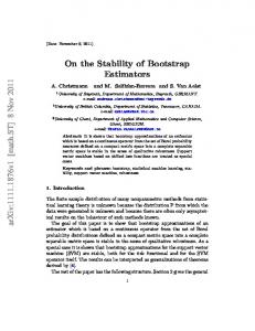
In the majority of sensory-performance measurements the typical finding is that the level of performance varies monotonically and nonlinearly with the level of the stimulus. In practice, the set of data relating stimulus level to performance level may be summarized by a single number, the critical level of the stimulus that yields a criterion level of performance. Thus when the response is discrete, referring say to the frequency with which a particular stimulus is detected, the critical level of the stimulus, in this case the threshold, may be defined as the level which corresponds to a detection frequency of 50 %. The performance function is often called the psychometric function (see Fig. 1a). In some situations, it may be possible to replicate the experiment and obtain several estimates of a parameter such as the threshold so that a mean value

may be calculated. The reliability of such a point estimate is then typically provided by the variance or standard deviation calculated from the set of individual estimates. But, in other situations, replication of the experiment may be impossible. Given a single set of performance data, an estimate of the standard deviation of a parameter estimate derived from the data set may then be essential in assessing the significance of the parameter estimate, either absolutely or in relation to parameter estimates derived from other distributions. Additionally, the estimate of standard deviation may have an importance in its own right, particularly when there may be sensory pathology (compare Patterson et al. 1980). When replication of the experiment is possible, estimates of the standard deviations of individual parameter estimates may still be useful in forming the best (minimum-variance) estimate of the mean or in assessing the contribution of potential outliers to the mean. Depending on the method used to fit a model sensory-performance curve to a single set of data, estimates of the variances of the parameters of the model may be derived by classical asymptotic theory. In particular, if ~ is the estimate of the parameter of interest, obtained as the solution of a maximumlikelihood equation, its estimated standard deviation SD is given by S"b = [ - l/(OZL/a T2)] ~/2,

where L is the likelihood and the partial derivative is evaluated at T. It is this relationship that is used to estimate the variance of the midpoint ("ED50") and of the slope in the classical probit-transformation approach to analysing psychometric functions (Finney 1964). Some computer software packages routinely produce estimates of the standard deviations of parameter estimates derived from the Hessian matrix of 2nd-order partial derivatives of the function describing the goodness of fit.

342 Little is known, however, about the trustworthiness of these asymptotic formulae when the sample size is small. Substantial errors are certainly possible. For example, biases in the estimated standard deviation of the slope of a fitted performance curve derived in a standard probit analysis may be 20-30 % for a fullrange (0-100%) curve, such as that in cases 1 or 3, Table 1, based on 25 trials or less, and may become many times larger for a half-range (50-100 %) performance curve, such as that in case 5, Table 1, based on 25 trials (see also McKee et al. 1985). Recently, Bradley Efron has developed a "bootstrap" method for estimating the standard deviation of a point estimate of a parameter, or any other aspect of its distribution (Efron 1982; Efron and Tibshirani 1986). In essence, the method entails approximating the theoretical distribution of the empirical observations by what Efron refers to as the bootstrap distribution. This distribution is obtained by taking the empirical distribution of the data in the definition of the parameter and then repeatedly sampiing the data, with replacement, to produce a Monte Carlo distribution of the resulting random variable. (A more formal definition is given in Sect, 2.) The bootstrap method has been found to be very powerful. It requires few modelling assumptions and little analysis, and can be applied automatically to almost any situation (Efron 1982), the success of the method depending on replacing traditional theoretical analysis by computing effort. The purpose of this report is to demonstrate the use of the bootstrap approach to the problem of estimating standard deviations of the estimated midpoints and spreads of sensory-performance functions based on small data sets. As will be shown, the bootstrap method appears well suited to dealing with small samples, and is dearly superior to general asymptotic methods.

2 Estimation of Standard Deviation by the Bootstrap Method Without loss in generality suppose that the performance measure is discrete, for example per-cent correct in a simple detection task, as illustrated in Fig. la. Let (I71, Y2,..., I~) be the observed set of 1 scores measured at levels xl, x2,..., xz of the stimulus. The scores Yieach represent the proportion of r~ successes out of n~ trials, i = 1, 2 .... , l, resulting from an unknown theoretical distribution F. Let 7" be the estimate of the parameter of interest (the midpoint ~, say) derived from the observed data by some procedure g; thus T=g(Y1, Y2 . . . . , Yt)-The standard deviation a(F, 7") of the statistic ~ cannot be written explicitly. Following

100

U

80

o o

60

c o o

40

12.

20 0

Ca.)

~-Model curve

_...4/

N=25 n.--5 i

I

-2.0

I

0.0 Stimulus

20

Sampleset

O

2.0 level, x

(b)

Bootstrap Normalcurve B=100

16

69 i-

mean=-0.204 sd=0.406

I2

chi2(9)=15.8

0 0

-2.0 Estimate

0.0

2.0

of mean, &

Fig. 1. a A performance curve based on a cumulative normal function EEq.(3a) with ~~ ~, c~= 0, fl= 1] and a sample data set based on 5 trials at each stimulus level x = - 2 , -1 ..... 2. b Histogram of values of the estimated midpoint a based on 100 bootstrap replications generated from the sample data set in a. The smooth curve is a normal curve with the same mean and standard deviation as the histogram

Efron (1982), we use a Monte Carlo algorithm. 1. Construct if, the empirical distribution of (Y1, Y2.... , Y~), i.e., the distribution obtained by placing the rescaled binomial Bi(ni, ri/n~)/ni, with ni draws and probability rJnf, at each level x~, i = 1, 2,..., I. 2. Draw a bootstrap sample (YI*, Y*,..., Yl*) from ff and calculate 7"* =g(Y1*, Y2*.... , Yl*)3. Independently repeat step 2 a large number B of times, obtaining bootstrap replications 7"'1 ~ . 2 ..... 7".B, and calculate [B~I

2-]1/2

where S'D=a(/?,~r~, the bootstrap estimate of the B

standard deviation of T,, and 7"*'= Z T*b/B. b=l

In the present Monte Carlo studies (Sect. 4), the number B of bootstrap replications was set at 100 (see

343

Efron 1982; Efron and Tibshirani 1986). Figure lb shows a histogram of values of the estimated midpoint generated from the sample data set shown in Fig. la.

method.

3 Estimation of Standard Deviation by the Incremental Method The performance of the bootstrap estimator of the standard deviation was assessed against an alternative, general estimator obtained by an approximate method belonging to the classical study of the "combination of observations". Like the bootstrap method it does not depend upon a particular theoretical model and it involves little analytic effort. Its application in the present context is described more fully in Foster (1986). With notation as in Sect. 2, consider the estimate T=g(Yx, Y2, .-., Yt), and suppose that the estimated variances ~2 of the Y~, i= 1, 2,..., l, are not too large. Then, provided that some additional conditions are satisfied (including the smoothness of g and the independence of the Y~),the estimated standard deviation g ~ is given approximately by

so=

E (Og/O )

(Y1, Y2,-.., Yz) (Foster 1986). The ~2 are given by the usual binomial formula Yi(1- Y~)/ni.It should be noted that if Y~=0 or I the i th term contributes nothing to SD. The method is also known as the incremental

,

(2)

i = 1

where the partial derivatives Og/OY~are evaluated at

4 Monte Carlo Studies

4.1 Data Simulation The bootstrap and incremental methods for obtaining the estimated standard deviation g'D were tested by applying them to simulated sensory-performance data generated in the following way. The underlying performance curve was assumed to be of the form of the traditional cumulative normal function

yi=l/7+(1-1/7)(2n) -1/z

exp

- ~ u a du,

--oo

z=(xi--~)/fl,

i = 1 , 2 .... ,1,

(3a)

where the constants ~ and fl define the midpoint of the curve and its spread [reciprocal of the slope at the midpoint except for the factor (1 -1/?)(2n)-1/2], and the constant y, when finite, corresponds to the number of alternatives in the MAFC task giving rise to the data. Thus, in the extreme, in a 2AFC task, the stimulus

^

Iog1013 3". "". ""i" Sample sets a=0

13=1

9 N=25 /'/.=5 1

-!

;Z,a t ,%.~: ...

- -,..~.

I -4

I -3

,| -2

-4t..

Q

g l ..e,. 9t J , ~ . ' :

"

." " ." :'. ":(':i:~'~" 9

.. " " / : . -

9 -1'

.r

:~.~.~

" . " .'1~9

!

2

I

I

3

4 Iogl0a

-t

Fig. 2.

P l o t of loglofl a g a i n s t l o g l o & Values of t h e e s t i m a t e d m i d p o i n t ~ a n d s p r e a d t , c o n s t r a i n e d to be positive finite, were o b t a i n e d f r o m t h e set of all d a t a sets (I"1, Y2,---, Ys) g e n e r a t e d by Eqs. (3) with ~ = 0, fl = 1, V ~ ~ , xi = - 2 , --1 .... ,2, a n d ni = n = 5 (as in Fig. la)

344 level x at the midpoint ~ corresponds to a performance level y of 75 %, and, in a "yes-no" task where 7 4 0% it corresponds to a performance level y of 50 %. Given ni trials at level x~, sequences of scores Y/were drawn from the corresponding rescaled binomial distributions Y~,-~Bi(n~, y~)/ni,

i = 1, 2 .... , I.

(3b)

In Fig. I a, the performance curve had constants c~= 0, fl = 1, and 7 4 0% and the data set was derived with x~= - 2, - 1,..., 2, and n i = n = 5. N o special significance should, however, be attached to the present use of the cumulative normal curve. Differences between it and the logistic function, also often used to model sensory-performance curves, are small over most of the range. F o r each set of simulated data (Ya, Y2 . . . . . Y~) generated by (3) for some ~, r, 7, xi, nz, i = 1, 2 ..... l, a curve of the form (3a) was fitted by maximizing the likelihood over c~and fl to obtain "new" estimates ~ and ft. Details of the estimation method are given in Foster (1986). With small data sets, there was an increased risk that values of ~ and fl for the fitted curve would take extreme values; in particular, c~could become positive infinite or negative infinite, and fl negative, zero, or positive infinite. It was not sufficient, however, to exclude just these values. Figure 2 shows, for positive finite values of ~ and r, values of loglo(fl~ plotted against values of log~o~ for the set of all data sets (]11, Y2,-.-, Yl) generated by (3) with ct=0, fl--1, 7 ~ o e , x~= - 2 , - 1 .... ,2, and ni = n = 5. The total number of points plotted is 1878. Despite the restriction of ~ and fl to positive finite values, there are a number of extreme values that would have a destabilizing effect on the computation of the standard deviation of the midpoint or of the spread of the distribution. To avoid this problem, sample data sets yielding values of ~ or fl greater than 20 times the range of the stimulus were excluded. F o r the case illustrated in Fig. 2, the range xs - x ~ was 4.0, and data sets were therefore excluded if either log 1o ~ or log~ o fi exceeded 1.9. The proportion of points thereby eliminated was 4.2 %. F o r a given set of constants c~,r, 7, x~, ni, i = 1, 2 .... , l, characterizing the model, either 5000 or 10000 such sets of admissible data were generated, in turn yielding either 5000 or 10 000 estimates of~ and ft. The standard deviations of these distributions were calculated and used as the "true" values of Sd(~) and Sd(fl~). 4.2

A s s e s s m e n t o f Standard-Deviation Estimators

The bootstrap and incremental methods were each tested by applying them to 1000 new "trial" sets

(Y1, Y2..... Yz) of simulated data, a set at a time, generated as above but independently of that exercise. A modification was made, however, to the implementation of the algorithms of Sects. 2 and 3. F o r a given trial set (Y~, Y2 .... , Y~),the model curve was fitted to the data, yielding estimates ~ and/7 for the midpoint and spread, and a replacement data set (Y~, Y~, ..., Yl') calculated, where Yi = Y~defined by (3a) with ~ = ~ and fl =/~ the other constants remaining unaltered. Each score in the original trial set was thus replaced by its "smoothed" value on the fitted curve 1. The algorithms were applied to these smoothed data sets. As noted earlier (Sect. 2), bootstrap estimates of the standard deviation were each based on 100 bootstrap replications. Because of the sensitivity of the bootstrap method to extreme values, each Monte Carlo distribution (of the estimates of the mean and of the spread) was symmetrically 2-fold Winsorized, that is, the values ~-,b in (1) were re-ordered linearly )-~.(1), ~.(2) .... ,~.(n), and ~-.(1), ~.(2) each replaced by ~.(3), and ~.(B),~.(B-~) each replaced by ~.w-2). Winsorization was essentially a safety measure, and, if omitted, would not have led to very large increases in estimated standard deviations 2. Winsorization was preferred to trimming, for in addition to imparting robustness it made some use of the extreme values. More serious difficulties due to extreme values would have arisen, however, if variances rather than standard deviations had been estimated from the empirical distributions. Winsorization was not applied to the distributions used to estimate the true values of Sd(~) and Sd(fl') (Sect. 4.l). Although these values were based on 5000-10000 draws, they may therefore have been vulnerable to occasional extreme values. For the incremental method, the partial derivatives in (2) were each estimated by finite-difference approximations, with averages of forward and backward differences being taken. The principal measure of performance of the bootstrap and incremental estimators g'DBooT and g'DINc for the parameters ~ = ~, fl was percentage bias, that is, the difference between the average of the 1 This parametric version of the bootstrap was employed to avoid obtaining spuriously small standard deviation estimates from data sets in which several of the Y~were zero or unity. Such data sets were particularly likely to occur when the total number of trials was small and stimulus levels were widely spaced z Without Winsorization, the worst biases in the estimates given in Table 1 were in case 1, where the bias in SDBoor(fl)iAncreased from 1.5% to 16%, and in case 2, where the bias in SDBooT(~) increased from 9 % to 26 %; all other biases were about the same as or less than those with Winsorization

345

The analysis was carried out for two different values of 7, two different numbers of levels l, and two different spacings of the levels, xl, x2,..., x~, the constants chosen to encompass typical experimental values. The values of the midpoint a, spread r, and number n, of trials at each level were kept fixed, a = 0, fl = 1, n, = 5, i-1,2,...,l. Computations were carried out in FORTRAN on two mainframe computers, a Cyber 176 and a CDC 7600, each with floating-point precision of 15 significant decimal digits. The NAG routine G05EYF was used to generate pseudorandom integers (Numerical Algorithms Group 1984).

estimate and the true value, expressed as a percentage of the true value, thus [(Ave(~'DBooT(T))-- S d ( ~ ) ) / S d ( T ) ] x 1 0 0 , and

[(Ave(g~xNc(7"))--Sd(~))/Sd(~)] x 100. Additionally, the relative efficiency of g"~BOOT with respect to ~ i N c was calculated as the inverse ratio of variances of the estimates, thus Var S(S(S~c(~))/Var S(S(S(~BOOT(7"))Although large data sets were not investigated here, it was confirmed in separate studies that ~BOOT and g'~iNc each behaved as consistent estimators 3.

4.3 Results Table 1 shows the results of the Monte Carlo studies. Summary data are given for the estimates ~'~(02) and ~'~(~) of the standard deviation of the estimated midpoint and spread, respectively, for the five different

3 For sufficiently large samples, the probability of the estimate being different from the "true" value could be made arbitrarily small; that is, for any small e > 0, prob {[ ~ ( N ) - S d ] > e}-~0 as N ~ o o , where N is the sample size

Table 1. Comparison of bootstrap and incremental methods of estimating standard deviations Of estimated midpoint c2and spread/~ of an underlying performance curve [Eq. (3)]. For each method, five Monte Carlo experiments were performed, each comprising 1000 trials (Y1, Y2.... , ~) distributed according to Eq. (3), with ~ = 0, fl = 1, ni = n = 5, and other constants as indicated. "True" values of the standard deviations were each based on 5000 or 10 000 trials. Relative efficiency of the bootstrap estimator was determined with respect to the incremental estimator Bootstrap estimate S"D~ooT(T) Ave

Std dev

Incremental estimate S'~rNc(T) %Bias

Rel Eft

Ave

True value Sd(T)

Std dev

%Bias

Curve range 0-100% (y~oo) Sample size ~ nl = N = 25 Model curve 1: number of levels l = 5, x i = - 2 , - 1 , 0, 1, 2 T=c~ 0.330 0.089 - 7.4 T=fl 0.320 0.202 1.5

0.89 0.76

Model curve 2: number of levels l = 5, x ~ = - 1, -0.5, 0, 0.5, 1 T= ~ 0.389 0.265 9.0 67 T=fl 0.799 0.740 -- 5.6 137

0.324 0.320

0.084 0.176

0.497 1.285

0.606 1.32

9.1 1.5

0.356 0.315

2.17 8.66

39.2 52.0

0.357 0.846

4.01 15.2

25.9 76.8

0.481 0.749

-

-

Curve range O-100% (7~oo) Sample size ~ nl = N = 15 Model curve 3: number of levels I=3, x ~ = - 1 , 0, 1 T=a 0.474 0.162 -- 1.4 T=fi 0.681 0.315 - 9.1

614 2336

Curve range 50-100% (7=2) Sample size ~ n~= N = 25 Model curve 4: number of levels 1= 5, x~= - 1 , -0.5, 0, 0.5, 1 T=c~ 0.552 0.255 -21.1 87000 T = fl 0.824 0.466 -- 27.7 278 000 Model curve 5: number of levels l = 5, x~=--2, --1, 0, 1, 2 T=a 0.779 0.385 -13.5 3100 T = fl 0.965 0.678 -- 19.9 12 200

10.6 35.2 1.99 5.18

75.2 246

1410 2990

0.700 1.140

21.4 74.8

121 330

0.900 1.200

346 model performance curves 4. Results have been divided according to curve range and sample size. The variations of the true values of the standard deviations (last column in Table 1) may be noted. Decreasing the number I of stimulus levels but keeping constant the spacing between levels and the number ni of trials performed at each level (cases 1 and 3) led to increases in the values of Sd(~) and Sd(fl~).Changing the value of so that the curve range contracted from 0-100% ("yes-no" task) to 50-100% (2AFC task) also led to increases the values of Sd(02) and Sd(/~~) (cases 1 and 5, and cases 2 and 4). Reducing the spacing between levels for 7 ~ ~ and for 7 = 2 (cases I and 2, and cases 5 and 4) had small but opposite effects, which presumably resulted from the introduction of respectively larger and smaller binomial variances at the altered stimulus levels. 5 Discussion The superiority of the bootstrap method is evident in Table 1. For all the full-range model curves (cases 1-3), percentage bias in ~'~BOOT(~) and S'DBoox(]~ ~) ranged from - 9 . 1 % to 9.0 %, including case 3 where the total number N of trials was 15. Percentage bias for the incremental method ranged from - 9 . 1 % to 76.8%, the latter occurring in case 3 for ~'D~c(~), although there were also large values in case 2. For the halfrange model curves (cases 4 and 5), the performance of both methods deteriorated, but much more seriously for the incremental method. For the bootstrap method percentage bias ranged from - 13.5 % to - 27.7 %, whereas for the incremental method it ranged from 121% to 2990%. The relative efficiency of the bootstrap method with respect to the incremental method was also generally high, particularly for the half-range model (cases 4 and 5) where values ranged from 3100 to 278 000. For bootstrap estimation with some parameters, for example the off-centre criterion level ED75, the distribution of the estimator may be sufficiently skewed that the standard deviation no longer provides an appropriate summary of its variability. Percentiles of the bootstrap distribution might then be used to estimate confidence limits for the true parameter value, although the number of bootstrap replications may have to be increased (Efron and Tibshirani 1986). It is worth emphasizing that the application of the bootstrap method to estimating the distributional characteristics of sensory-performance functions is not tied to the use of either the cumulative normal curve (3a) or the binomial distribution (3b). The method 4 Averagevaluesof ~*"and/~*"did not differfromtheir "true" values bymore than 0.009and 0.094respectivelyin cases1-3, and by more than 0.163 and 0.211 respectivelyin cases 4 and 5

should be equally useful for other sigmoidal performance functions, including the logistic function, and, more generally, the power-law increment-threshold function (Foster 1986). Although not explored here, a characteristic consequence of using the bootstrap method (or any Monte Carlo method) to analyse an individual set of empirically generated data is that replication of the analysis need not yield precisely the same value of the estimated standard deviation. Provided that the model curve is an appropriate representation of the underlying performance and that the relative efficiencies given in Table 1 offer a reliable guide, the differences in these values should be small. Simulation errors can of course be reduced by increasing the number B of bootstrap replications, or by introducing techniques that increase the efficiency of the simulations (e.g., Davison et al. 1986). The numbers of trials associated with each model curve were here constrained to range from 15 to 25. Most experimental designs (including fixed-levels methods and adaptive procedures such as PEST; Taylor and Creelman 1967, and hybrid PEST; Hall 1981) would usually specify more than 25 trials overall, but there are some circumstances where it may be possible to perform only a few trials, for example, when estimating a threshold or spread for a sensory system whose characteristics are changing fairly rapidly, as in some sensory-adaptation paradigms, or when for other reasons there is little time for measurement, as in some clinical situations. Bootstrap estimation of the standard deviations of these parameters appears to offer an acceptably reliable method of assessing their significance. A F O R T R A N listing of the main programs used in this study is available from the first author on written request.

Acknowledgements. We thank A. C. Davison, A. M. Herzberg, and S. R. Pratt for critical review of the manuscript. WFB was supported by Grant No. 81.166.0.84 from the Swiss National Science Foundation. References Davison AC, Hinkley DV, Schechtman E (1986) Efficientbootstrap simulation. Biometrika 73:555-566 Efron B (1982) The Jackknife, the bootstrap and other resampling plans. CBMS-NSF Regional Conference Series in Applied Mathematics, No. 38; Philadelphia, PA, Societyfor Industrial and Applied Mathematics Efron B, Tibshirani R (1986) Bootstrap methods for standard errors, confidenceintervals, and other measures of statistical accuracy. Statist Sci 1:54-75 Finney DJ (1964) Probit analysis. Cambridge University Press, Cambridge

347 Foster DH (1986) Estimating the variance of a critical stimulus level from sensory performance data. Biol Cybern 53:189-194 Hall JL (1981) Hybrid adaptive procedure for estimation of psychometric functions. J Acoust Soc Am 69:1763-1769 McKee SP, Klein SA, Teller DY (1985) Statistical properties of forced-choice psychometric functions: implications of probit analysis. Percept Psychophys 37:286-298 Numerical Algorithms Group (1984) FORTRAN library manual, Mark 11, vol 5. Numerical Algorithms Group, Oxford Patterson VH, Foster DH, Heron JR (1980) Variability of visual threshold in multiple sclerosis. Effect of background luminance on frequency of seeing. Brain 103:139-147

Taylor MM, Creelman CD (1967) PEST: Efficient estimates on probability functions. J Acoust Soc Am 41:782-787

Received: May 29, 1987

Dr. D. H. Foster Department of Communication and Neuroscience University of Keele Keele Staffordshire ST5 5BG United Kingdom

Verantwortlich fiir den Textteil: Prof. Dr. W. Reichardt, Max-Planck-Institut fiir biologische Kybernetik, Spemannstr. 38, D-7400 Tiibingen. Verantwortlich f'tir den Anzeigenteil: E. L/iekermann, Springer-Verlag, Heidelberger Platz 3, D-1000 Berlin 33, Fernsprecher: (030)8207-0, Telex: 01-85411. 9 Springer-Verlag Berlin Heidelberg 1987. Druck der Briihlschen Universit~itsdruokerei, Giel]en. Printed in Germany. - Springer-Verlag GnabH & Co KG, 1000 Berlin 33