Electronic version of an article published as Advances in Complex Systems, doi: 10.1142/S0219525912500786 c World Scientific Publishing Company, http://www.worldscientific.com/worldscinet/acs
BOOTSTRAPPING PERCEPTION USING INFORMATION THEORY: CASE STUDIES IN A QUADRUPED ROBOT RUNNING ON DIFFERENT GROUNDS
NICO M. SCHMIDT Artificial Intelligence Laboratory, Department of Informatics, University of Zurich, Andreasstrasse 15, 8050 Zurich, Switzerland
[email protected] MATEJ HOFFMANN
[email protected] KOHEI NAKAJIMA
[email protected] ROLF PFEIFER
[email protected] Received 21 February 2012 Revised 23 May 2012 Accepted 29 May 2012 Animals and humans engage in an enormous variety of behaviors which are orchestrated through a complex interaction of physical and informational processes: the physical interaction of the bodies with the environment is intimately coupled with informational processes in the animal’s brain. A crucial step toward the mastery of all these behaviors seems to be to understand the flows of information in the sensorimotor networks. In this study, we have performed a quantitative analysis in an artificial agent - a running quadruped robot with multiple sensory modalities - using tools from information theory (transfer entropy). Starting from very little prior knowledge, through systematic variation of control signals and environment, we show how the agent can discover the structure of its sensorimotor space, identify proprioceptive and exteroceptive sensory modalities, and acquire a primitive body schema. In summary, we show how the analysis of directed information flows in an agent’s sensorimotor networks can be used to bootstrap its perception and development. Keywords: information theory; transfer entropy; perception; developmental robotics; sensorimotor contingencies; body schema;
1. Introduction Animals are constantly being confronted with a massive multidimensional flow of information that is sampled by their receptors and, after some preprocessing, relayed 1
2
NICO M. SCHMIDT et al.
to their brains. This information has to be processed for the animal to be able to take the right decisions and execute the actions that maximize its chances of survival. In addition, the organism and the environment are dynamically and reciprocally coupled and so are the sensory and motor signals. It is the sensorimotor networks (as opposed to purely sensory information) and the dynamic patterns that exist in them that provide the basis for further processing. Cognition is then best viewed as emerging from this dynamic sensorimotor coupling (e.g. [39, 26]). The view just described holds for natural and artificial agents (i.e. animals and robots) alike. Robots - if they are to autonomously succeed in the real world - also need to extract the relevant information about their interaction with the environment. In order to understand the nature of the processing that is responsible for cognition, the prerequisite seems to be to quantify and analyze the structure of the information flow in these sensorimotor networks. The tools of information theory such as entropy, mutual information, integration, complexity and transfer entropy have proven useful in this respect. They have been applied to inspect information flows inside the brain (e.g. [8, 37, 11, 9]), as well as in the data collected from robots. Lungarella and Sporns [20] have conducted studies on robots that illustrate the effect of individual components of the sensorimotor loop on the information structure. In particular, they showed how a given sensorimotor coordinated behavior (such as foveation) can increase the information content that reaches a given sensor (an artificial retina). Manipulating the sensor morphology (log-polar transformation in this case) showed similar effects. Williams and Beer [41] conducted an informationtheoretic analysis of a simple agent engaged in a categorization task. Nakajima et. al. [22] showed how directed information flow, measured by symbolic transfer entropy can help to characterize the force-propagation in an artificial octopus arm. The bulk of the work described so far was adopting a largely descriptive perspective - given a behaving system (a brain, or a complete agent with sensors and actuators), the information flow and structure was analyzed. We have argued above that this is a key step to understand the behavior of the system. However, an alternative perspective is to look at the world through the eyes of the agent itself. Imagine an animal or robot has just been “born”. Using its actuators, it can interact with the world, generating sensory stimulation. Without prior knowledge of its body, sensory apparatus, and the surrounding environment, how can it make sense of the sensorimotor signals it is experiencing? As the agent interacts with the environment, it will experience some patterns (regularities, contingencies) much more often than others - this is given by the agent’s embodiment, the morphology and material properties of its body and the placement of its sensors ([14] provide an overview of case studies illustrating these effects). Remembering or representing those regularities will be useful to the agent. But where should the agent start? We think that it should start at the very basis: it should first learn the extent of its body, the things it can influence and what lies beyond its control and should be attributed to the environment. Such a process has been observed in infants who spend substantial time in
BOOTSTRAPPING PERCEPTION USING INFORMATION THEORY
3
their early months observing and touching themselves [33]. Through this process of babbling, intermodal redundancies, temporal contingencies, and spatial congruences are picked up. In such a process, the infant forms a model of its body (a body image or body schema, see e.g. [4, 3, 21]). A developmental approach can also be applied to robots [19, 40, 27]. To identify its own body and learn about its contingencies is a natural candidate to start the autonomous development in an artificial agent (see [13] for a review on self-models and their acquisition in robots). Several studies along those lines have been conducted: typically, they involve an upper torso humanoid robot that is observing the space in front of it with a camera. The goal is to identify the parts of the visual scene that belong to its body (its arms, for instance). Different assumptions can be employed: the robot is static and environment is varied [43], or, on the contrary, temporal contingency is exploited by the robot - the robot learns to recognize its body parts by moving them [7, 23, 10]. Some researchers attempt to start with even less prior knowledge: Olsson et al. [24, 25] and Philipona et al. [30] study cases, where the agent is confronted with raw uninterpreted sensory signals only. There is no preprocessing, no knowledge of geometry and the agent does not even know which signals come from which modality. In [30] a simple simulated agent learns to make the distinction between body and environment by observing over which part of the sensory channels it has complete control. Olsson et al. [24, 25] have collected data from a real robot and showed that using an information metric as distances between the sensory and motor channels, the robot is able to reveal the (mainly spatial) relationships from its morphology (eg. arrangement of camera pixels). Our work is very much in line with the approach of Philipona et al. [30] and Olsson et al. [24, 25]. For our study, we have chosen a running quadruped robot with the following modalities: four motor signals, eight angular position sensors (4 on active and 4 on passive joints), 4 pressure sensors on the robot’s feet, a 3-axis accelerometer and 3-axis gyroscope. The control signal and the environment (five different ground materials) are systematically varied and the sensorimotor data is collected. The information flows are analyzed using transfer entropy and the effect of the different conditions is investigated. Then, we adopt the perspective of the autonomous agent and show how the agent can use the information flows to: (1) derive a primitive body schema and infer the controllability of different sensory variables; (2) discriminate different environments; (3) discover the structure of its sensorimotor space (identify proprioceptive and exteroceptive modalities, group different modalities and extract topological relations); and (4) interpret the quantity of information flow to assess the utility of different sensory channels and its overall performance. This article is structured as follows. In Sec. 2, we will first introduce the information theoretic methods used and the experimental setup. In Sec. 3, we report on the results of the experiments. A brief section desribing the robot’s behavior from an observer perspective is followed by a detailed analysis of the information
4
NICO M. SCHMIDT et al.
flows under different conditions and their implications for the robot’s autonomous development and perception. The paper is closed by a discussion, followed by a final conclusion and suggestions on future work. 2. Materials and Methods In this section, we describe the information theoretic measures used, our experimental setup, and explain in detail how we analyzed the data in this paper. 2.1. Information Theoretic Measures: The Transfer Entropy We use the term information in the Shannon sense, that is, to quantify statistical patterns in observed variables. Thus, the measures presented here are based on Shannon entropy [2]. Given a time series xt from the system X, entropy H(X) provides a measure of the average uncertainty, or information, calculated from the probability distribution p(xt ) according to: X H(X) = − p(xt ) log p(xt ). (1) xt
The association between two time series is often expressed as their mutual information XX p(xt , yt ) I(X; Y ) = p(xt , yt ) log . (2) p(x t )p(yt ) x y t
t
which expresses the deviation from the assumption that both are independent from each other. However, mutual information also contains information that is shared by X and Y due to a common history and it is invariant under exchange of the two variables. As we were interested in characterizing the directed information flow between the time series, we used transfer entropy [34], which provides this directionality and removes the shared information. Transfer entropy was introduced to measure the magnitude and the direction of information flow from one element to another and has been used to analyze information flows in real time series data from neuroscience [9, 11], robotics [38, 22], and many other fields. Given two time series X and Y , the transfer entropy T E essentially quantifies the deviation from the generalized Markov property p(xt+1 |xt−τ ) = p(xt+1 |xt−τ , yt−τ ) [34]. If the deviation is small, then Yt−τ can be assumed to have little relevance on the transition from Xt−τ to Xt+1 . If the deviation is large, however, then Yt−τ adds information about the transition of Xt−τ and the generalized Markov property is not valid. The deviation from this assumption can, similar as in the mutual information, be expressed as a specific version of the Kullback-Leibler divergence: X X X p(xt+1 |xt−τ , yt−τ ) p(xt+1 , xt−τ , yt−τ ) log (3) T Eτ (Y → X) = p(xt+1 |xt−τ ) x x y t+1
t−τ
t−τ
where the sums are over all possible states, t is the current time step and τ ∈ N0 indicates the time lag of the transition.
BOOTSTRAPPING PERCEPTION USING INFORMATION THEORY
5
In other words, T E measures how well we can predict the transition of the system X by knowing the system Y , beyond the degree to which X already disambiguates its own future. Transfer entropy is non-negative, any information transfer between the two variables resulting in T E ≥ 0. As proposed by Williams & Beer [42], the transfer entropy can be decomposed in two different kinds of information transfer, the state-dependent transfer entropy (SDT E) and the state-independent transfer entropy (SIT E). The former characterizes the information transfer that is caused by the synergy of both variables in predicting the transition from Xt−τ to Xt+1 , so it not only depends on Yt−τ , but also on the state of Xt−τ . The latter kind of information transfer is the unique information that Yt−τ yields about Xt+1 and is completely independent from Xt−τ . Moreover, in control theoretic terms the SIT E expresses the open-loop controllability of a variable X by its controller Y , while the SDT E expresses the Y ’s closed-loop controllability of X [42]. The state-dependent and state-independent transfer entropy are defined as SIT Eτ (Y → X) = I(Xt+1 ; Yt−τ ) − Imin (Xt+1 ; Yt−τ , Xt−τ ) SDT Eτ (Y → X) = I(Xt+1 ; Yt−τ , Xt−τ ) − Imax (Xt+1 ; Yt−τ , Xt−τ ) T Eτ (Y → X) = SIT Eτ (Y → X) + SDT Eτx (Y → X) where Imin is defined as: Imin (Xt+1 ; Yt−τ , Xt−τ ) =
X
p(xt+1 )
xt+1
min
R∈{Yt−τ ,Xt−τ }
I(Xt+1 = xt+1 ; R)
(4) (5) (6)
(7)
and Imax is defined the same way except substituting min with max. In order to remove the bias due to the statistical properties of the time series, and in order to make the information transfers between different signals comparable, we subtract the shuffled information transfer and normalize it to the range [0, 1] according to [11]. The shuffled information transfer is calculated by first scrambling the data of the time series Y so that the time-dependency is lost but the statistical properties remain. The normalized transfer entropy is then expressed as: T Eτ (Y → X) =
T Eτ (Y → X) − T Eτshuf f led (Y → X) H(Xt+1 |Xt−τ )
(8)
2.2. Experimental Setup The experimental setup was identical to our previous work [32]. We recapitulate it here for the reader’s convenience. 2.2.1. Robotic Platform and Control Signals The robot used (Fig. 1 (a)) had four identical legs driven by position-controlled servomotors in the hips. It had passive compliant joints at the knees. Upper and lower limb were connected with springs. A special material (adhesive skin used for
6
NICO M. SCHMIDT et al.
ski touring from Colltex), which has asymmetrical friction properties, was added onto the robot’s feet. This allowed the robot to get a good grip during leg retraction (stance), and enabling sliding during protraction (swing). The mechanical design (weight distribution, proportions, springs used, etc.) was a result of previous research (e.g. [16]).
(a)
(b)
Arena
Robot Inertial measurement unit 㽢1 Hip-joint sensor 㽢4 Knee-joint sensor 㽢4 Foot pressure sensor 㽢4 Fig. 1. Robot experiments. (a) The quadruped robot “Puppy” with its set of sensors (colored circles). (b) The arena used in the experiments (linoleum ground shown). The picture was taken from an overhead camera which was used to track the robot trajectories.
We prepared three sets of position control commands for the servomotors, resulting in three distinct gaits. The first one was the random gait, where the target hip joint angle for each leg was set randomly with certain smoothing constraints (to avoid too high frequencies that would exceed the motor bandwidth). The remaining two gaits were based on a simple oscillatory position control of the motors, each motor signal a sine wave. The target hip joint angle γi of each motor i (and hence of each leg) was determined as γi (t) = αi · sin(2πf t + θi ) + βi ,
(9)
where the oscillation was varied by changing the amplitude αi , offset βi , frequency f , and phase lag θi parameters. Offset βi defines the center of the oscillation. In the experiments reported here, frequency f of all legs was set to 1 Hz. By experimentation, we have prepared two parameter settings which gave rise to two turning gaits. The bound right gait was derived from a bounding gait; the turn left gait achieved the left turn by simply using a higher amplitude in the hind right leg. The motor signals of the three gaits are shown in Fig. 2.
Motor Signals [rad]
BOOTSTRAPPING PERCEPTION USING INFORMATION THEORY random
bound right
turn left
time [s]
time [s]
time [s]
7
0.5
0
−0.5
−1
FL FR HL HR
Fig. 2. Motor time series. The plots show 3.5 s of the motor commands as the robot runs with random, bound right and turn left gait respectively. The signals are shown for every leg, FL: front left, FR: front right, HL: hind left, HR: hind right.
Besides the four motor channels (denoted as MF L ,MF R ,MHL ,MHR ), we used 18 sensory channels from the robot (see Fig. 1 (a)). Eight potentiometers were used to measure the joint angles, four on the active hip joints (HF L ,HF R ,HHL ,HHR ) and four on the passive knee joints (KF L ,KF R ,KHL ,KHR ). On the robot’s feet were four pressure sensors (PF L ,PF R ,PHL ,PHR ). Linear accelerations in three axes (AX ,AY ,AZ ) and angular velocities around the three axes (GX ,GY ,GZ ) were taken from an inertial measurement unit (IMU). All sensory data were sampled at 50Hz. For convenience, we refer to the hip and knee angular sensors as “hips” and “knees” and speak about “motors” when we mean the motor commands. 2.2.2. Arena and Ground Conditions During the experiments, the robot was running in an arena roughly 2.5 x 2.5 m and was tethereda (Fig. 1 (b)). The turning gaits were chosen to keep the robot inside the arena. To investigate the effect of ground conditions, we used five different ground materials: linoleum, foil, cardboard, styrofoam and rubber. The main difference was in the friction coefficient between the ground material and robot’s feetb In addition, the rubber and cardboard contained regular ridges. 2.2.3. Experiments As we have discussed in Sec. 1, behavior is an outcome of the dynamical reciprocal coupling of the brain, body and environment. Fig. 3 illustrates this schematically. All the interacting components introduce some constraints on the interplay and a Cables
were used for data transfer and power transmission. Although they did affect the robot’s dynamics, an effort has been made to minimize these effects by carrying the cables by the experimenter. b We estimated static friction coefficients by putting a block covered with the same adhesive skin as on the robot’s feet on inclined planes covered with the different ground materials. As the adhesive skin has asymmetrical properties, two values were obtained for each material. The low/high values were: linoleum: 0.31/0.40, foil: 0.39/0.39, cardboard: 0.64/1.10, styrofoam: 0.74/1.06, rubber : 0.76/0.91.
8
NICO M. SCHMIDT et al.
together induce some regularities or structure. Adopting the situated perspective, we will study how much can be inferred by the agent about the interaction from observing the sensorimotor flows only. To this end, we have designed experiments in which two of the interacting components are systematically varied.
Fig. 3. The interplay of information and physical processes. Driven by motor commands, the mechanical system of the agent acts on the external environment (different ground substrates in our case). The action leads to rapid mechanical feedback (for example, springs in the passive knees are loaded). In parallel, external stimuli (pressure on the robot’s feet or acceleration due to gravity) and internal physical stimuli (bending of joints) impinge on the sensory receptors (sensory system). The arrows marked with ellipses correspond to the information flows that are available to the agent’s “brain” for inspection; these are the subject of our analysis. Figure and text adapted from [29].
Experiment 1: Varying the controller. We have varied the control signals sent to the robot’s motors, which give rise to disctinct gait patterns. A set of random signals (random) and two coordinated motor controllers (bound right and turn left) were prepared. Keeping the body and environment constant (linoleum ground was used), we investigated how the information structure changes with the different controllers. Experiment 2: Varying the environment. By fixing the controller to the bound right gait, we investigated how the ground conditions affect the informational structure experienced by the robot. For the ground conditions, we used foil, linoleum, cardboard, styrofoam and rubber.
BOOTSTRAPPING PERCEPTION USING INFORMATION THEORY
9
The body was not varied in our experiments. However, as the other main actors - the control signals and the environment - were systematically manipulated, it was to some extent possible to investigate its effect by uncovering the invariant (always present) structure in the sensorimotor space. 2.3. Data Analysis The trial durations of the experiments were between 60 and 130 seconds. To have an equal number of samples for the calculations of the information transfer, we divided longer trials into subtrials of 58s length (2900 samples). Additionally, we discarded the first 2 seconds (100 samples) of each trial, in order to exclude the data of the transition from sitting to running. This way we obtained between 2 and 5 subtrials per condition. The marginal and joint probability distributions that were needed to calculate the information flows were estimated using histograms. After normalizing the time series to a standard normal distribution (X, Y ∼ N (0, 1)), the state space was divided into 20 equally spaced bins ranging from [-4, 4] and the frequency of each state was counted. We tried different bin numbers (5 to 64) and ranges and observed no qualitative difference in the resulting information transfer. The information transfer was then averaged over all trials in each condition. We calculated them for time lags τ = [0, 1] seconds (1 second was the period of locomotion of the robot) and selected the maximum across τ = argmaxτ [T Eτ (Y → X)]. The shuffled information transfer used for the normalization was calculated by scrambling the time series of Y 100 times, then calculating the information transfer for all 100 scrambled time series and taking the mean of that. 3. Results In this section, we start by briefly looking at the behavior of the quadruped robot in the arena from an observer perspective. Then we will analyze the information structure that can be extracted from the time series. We will see how the behavior is reflected in the information structure and how it can contribute to the robot’s perception and development. We also would like to draw the reader’s attention to a video from the experiments that will provide a clearer picture of the experimental conditions in which the robot interacts with its environment: https://files.ifi.uzh.ch/ailab/people/hoffmann/videos/ ACS2012/SchmidtEtal_ACS_2012_accompVideo.mpg or .wmv. 3.1. Behavior Fig. 4 (a) compares example trajectories of the robot for the three different gaits on the linoleum ground. We can clearly see that the robot’s behavior was different in each gait. Interestingly, we found that for the random gait the robot moved forward and had a tendency to turn clockwise (light gray line). Since the motor signal was random, we attribute this pattern to the asymmetry in the morphology
10
NICO M. SCHMIDT et al.
of the robot. The forward motion can be attributed e.g. to the mass distribution, the leg shape, and the asymmetric friction properties of the adhesive skin on the robot’s feet. The turning effect could be explained by the IMU attachment with the cable pointing to the right. In the turn left gait, the trajectories of the robot showed counterclockwise circles (dark gray line). From the pronounced “zig-zag” shape - as seen by the overhead camera - we can also observe that the robot’s rolling motion was substantial and larger than the forward motion of the robot in each locomotion period. In the bound right gait, the robot turned clockwise (black line). The diameter of the trajectory seemed to be modulated by the ground type (Fig. 4 (b)). In particular, if the friction between ground and feet was larger, the diameter of the circle was smaller. In summary, the robot showed a characteristic behavior for each gait condition (controller) and its behavior is strongly affected by the ground type (environment). Gaits
a)
b)
Grounds
bound right (40s) turn left (40s) random (40s)
foil (30s) styrofoam (30s) linoleum (30s) cardboard (30s) rubber (30s) Start
Start
20cm
20cm
Fig. 4. Robot trajectories. Typical trajectories of the robot’s center of mass in the arena, as viewed from above. (a) The trajectories on the linoleum ground when running with bound right (black), turn left (dark gray) and random (light gray) gait. (b) The trials from different grounds with the bound right gait. The trajectories also reveal how the turning radius and the distance traveled (the speed of the robot) was dependent on the ground condition.
3.2. Experiment 1: Influence of the Controller on the Information Structure 3.2.1. The Random Controller and Body Schema Synthesis We start by analyzing the random controller, in which the motor commands were set randomly and independently so that there was no correlation among them. If we let the robot run long enough, in the limit we will encounter all possible
BOOTSTRAPPING PERCEPTION USING INFORMATION THEORY
11
combinations of motor commands of the four legs. The random controller can then be seen as marginalizing out the controller part of the controller-body-environment system. Hence, information structure obtained with this gait can be considered to be induced by the interaction between the body and the environment of the robot only. Fig. 5 shows the transfer entropy among all the variables in the linoleum ground condition. A cell of the matrix (a) indicates the information transfer from the signal in the column to the signal in the row.
linoleum - random
GZ GY GX AZ AY AX PH R PH L PF R PF L KH R KH L KF R KF L HH R HH L HF R HF L
0.4
0.35
0.3
0.25
0.2
[bits]
a)
0.15
0.1
MF L MF R MHL MH R HF L HF R HH L HHR KF L KF R KHL KH R PF L PF R PHL PHR AX AY AZ GX GY GZ
0.05
0
Fig. 5. Transfer entropy T E in the random gait on linoleum. (a) Every cell of the matrix corresponds to the information transfer from the signal on the column position to the signal on the row position. (b) A schematic of the Puppy robot (dashed lines) with overlaid arrows depicting the T E between the individual components. For readability, only the 15 highest values are shown and the accelerometers and gyroscopes were excluded from this visualization. The strength of the information transfer is encoded as thickness and color of the arrows.
The strongest information transfer occurs from the motor signals to their respective hip joint angles (MF L → HF L , MF R → HF R , MHL → HHL , MHR → HHR ). The motors directly drive the respective hip joints and, despite some delay and noise, the hip joints always follow the motor commands, which induces a strong informational relation. The motors further show a smaller influence on the knee angles (especially at the hind legs KHL and KHR ) and on the feet pressure sensors, all on the respective leg where the motor is mounted. Finally, also the hip joints have some weak influence on the pressure sensors of the respective leg. The schematic of the Puppy robot in Fig. 5 (b) shows the same information flows as arrows with thickness and color depicting the strength of information transfer between the components (sensors from the IMU are not shown in this schematic). It can be seen that the information is mainly propagated within each leg, with stronger flows in the hind legs. Other interesting relations revealed by the transfer entropy are between AY and GX , and between AX and GY . These reflect the robot’s pitching and rolling movements, respectively, which are prominent motions in the quadruped robot.
12
NICO M. SCHMIDT et al.
When the robot rolls to one side, the gyroscope measures angular velocity around the X-axis (GX ), while the acceleration due to gravity partly projects into the Y component, appearing in AY . Similarly the pitching movement affects the sensors AX and GY . Concluding, while the overall information in the gait induced by the random controller is quite low, the few relations that stick out reflect many things we know about the robot’s physical structure and its behavior. In particular, the information flows between sensors and motors of the same leg are prominent, and the rolling and pitching movements induce flows between accelerometers and gyroscopes. We propose that the contingencies derived from this gait constitute a rudimentary body representation of the robot. Of course this body schema is only valid in the environment the robot has experienced during the trials (linoleum in this case, but could be extended to all available ground conditions). We want to emphasize that contrary to the work in robotics dealing with self-recognition or self-calibration that we have reviewed in Sec. 1, the agent can arrive at this model with minimal assumptions or prior knowledge.
3.2.2. Coordinated Motor Commands In the following, we will see how the information structure changes if we introduce controllers with coordinated, synchronized motor commands, which give rise to the bound right and turn left gait. The motor commands in these gaits are periodic oscillatory signals of the same frequency, but of different amplitudes, offsets and phase. Consequently, the robot exhibits periodic behavior and periodic-like signals are induced in the sensory channels. From Fig. 6 (a, c) we see that the overall amount of information transfer is much higher than with the random controller. Furthermore, the information transfer no longer occurs only among the variables within one leg, but also among variables belonging to different legs. In the bound right gait (a, b), all motors (M ) transfer much information to all hip joints (H). The knee joints receive as much information from the motors as the hip joints. In the turn left gait (c, d), on the other hand, the strongest influence of the motors is on the hind right hip (HHR ), followed by the hind knees. The pressure sensor PHR receives more information than the other pressure sensors and the flows among different hip joints are very low except for the flows from the HHR to the others. The special role of the hind right leg in the flows reflects the fact that the MHR motor has a much higher amplitude and is a key contributor to the robot’s locomotion (cf. video). The information flows from the motors to the inertial sensors can be also related to the behavior displayed by the two gaits. The high flows from the motors to GY in the bound right gait relate to the pitching movement. The trajectories as observed by the overhead camera (Fig. 4 (a)) show a pronounced sidewards “zig-zag” movement during the turn left gait. This corresponds to the roll motion which is reflected in
BOOTSTRAPPING PERCEPTION USING INFORMATION THEORY
linoleum - bound right
GZ GY GX AZ AY AX PH R PH L PF R PF L KH R KH L KF R KF L HHR HHL HF R HF L
0.55 0.5 0.45 0.4 0.35 0.3 0.25
[bits]
a)
13
0.2 0.15 0.1
MF L MF R M HL MHR HF L HF R HHL HHR KF L KF R K HL KH R PF L PF R P HL P HR AX AY AZ GX GY GZ
0.05
linoleum - turn left
GZ GY GX AZ AY AX PH R PH L PF R PF L KH R KH L KF R KF L HHR HHL HF R HF L
0.55 0.5 0.45 0.4 0.35 0.3 0.25
[bits]
c)
0.2 0.15 0.1
MF L MF R M HL MHR HF L HF R HHL HHR KF L KF R K HL KH R PF L PF R P HL P HR AX AY AZ GX GY GZ
0.05
Fig. 6. Transfer entropy in the coordinated gaits on linoleum. The matrices and Puppy schematics show the transfer entropy in the bound right gait (a,b) and the turn left gait (c,d) in the same way as described in Fig. 5. Please note the different scale of the matrices and the Puppy schematics.
the high flows from the motors to AY and GX . All these examples show that the measured information flows strongly reflect aspects of the robot’s behavior and the physical properties of its body. Furthermore, they show that periodic behavior induces specific informational structure through synchronization.
3.2.3. Controllability Can maps of sensorimotor flow be utilized for control purposes, i.e. to achieve desired states or goals by the robot? As stated in Sec. 2.1, the transfer entropy from a controller to a variable expresses the controllability of this variable. Moreover, the decomposition into state-independent and state-dependent transfer entropy (SIT E and SDT E) allows to distinguish the open-loop and closed-loop controllability of the variable. This means the agent can infer the controllability of its sensory channels by its motors by looking at the flows from its actuators to its sensors. Fig. 7
14
NICO M. SCHMIDT et al.
shows this decomposed directed information transfer for the three sets of motor commands used in the Puppy robot. Part a) - from the random controller - hints on the controllability of the platform in general. We see that the hip joints can be controlled by the motors in the respective leg and there is indication that this can be done in an open-loop fashion, since the SIT E component is stronger c . The flows to the knee and pressure sensors, in particular in the hind legs, also hint on their possible controllability in an open-loop fashion. Fig. 7 b) and c) depict the situation of the coordinated gaits. The information flows indicate higher open-loop controllability of the hips and the pressure sensors (stronger SIT E part). Although we saw in the previous section that in the coordinated gaits the knees receive more total information from the motors than the hips, the decomposition shows that this mainly comes from the SDT E – their closed-loop controllability. So in order to control the knees, the feedback about their current state may be needed.
SITE
MFL MFR MHL MHR MFL MFR MHL MHR
c)
SDTE
GZ GY GX AZ AY AX PHR PHL PFR PFL KHR KHL KFR KFL HHR HHL HFR HFL
turn left SITE
SDTE
GZ GY GX AZ AY AX PHR PHL P FR P FL KHR KHL KFR KFL HHR HHL HFR HFL
0.5 0.45 0.4 0.35 0.3 0.25
[bits]
b) bound right
SDTE
0.2 0.15 0.1 0.05
MFL MFR MHL MHR MFL MFR MHL MHR
random SITE
GZ GY GX AZ AY AX PHR PHL PFR P FL KHR KHL KFR KFL HHR HHL HFR HFL
MFL MFR MHL MHR MFL MFR MHL MHR
a)
0
Fig. 7. Decomposition of the transfer entropy. The matrices show the decomposition of the information flows observed from the three controllers into SIT E and SDT E. Only the flows from the motors to the sensors of the robot are shown.
What would be the first goal-oriented behaviors that would be meaningful in the current situation? Let us imagine that the robot “wants” to accelerate forward or to turn. That is, a desired sensory state would be a high value of AX or GX respectively. From the information flows, we see that AX is more affected by the motors in the bound right gait, whereas for GX , it is the turn left gait that shows a stronger flow. The robot could thus choose a gait that would make the desired control action easier. Then, to obtain a simple controller, we would be interested in the “inverse” mapping - from the sensory variable to the motor signal - that would c In
reality, every hip is controlled with a closed-loop controller of the servomotor. However, this is hidden from the robot and hence, from a situated perspective, it is plausible to assume that they can be controlled in open-loop.
BOOTSTRAPPING PERCEPTION USING INFORMATION THEORY
15
give us appropriate motor commands. This mapping could then be worked out as a functional relationships using regression, for example. 3.3. Experiment 2: Influence of the Environment on the Information Structure In experiment 2 we let Puppy run with the bound right gait on five different grounds to investigate how the interaction with different environments changes the information structure. 3.3.1. Ground Discrimination Fig. 8 shows the standard deviation of the information flows across the five ground conditions (after averaging the trials within the ground conditions). It reveals which flows are sensitive to changes of the ground and which remain constant. The matrix (a) shows that especially among motors and hip joints the relations are very strong and invariant to ground changes. On the contrary, the information that the hind left pressure sensor PHL receives from many of the other channels, is very dependent on the ground condition, which can be seen from the arrows to PHL in (b). We can again see that the flows reflect some properties of the robot’s body: the hips follow the strong motors and are largely unperturbed by variations of the environment, while the pressure sensor measures directly the ground contact and can sense the differences (especially the hind left one, which takes the highest load during forwardrightward pushing in this gait). Std over grounds
GZ GY GX AZ AY AX PH R PH L PF R PF L KH R KH L KF R KF L HHR HHL HF R HF L
0.14
0.12
0.1
0.08
[bits]
a)
0.06
0.04
MF L MF R M HL M HR HF L HF R HHL HHR KF L KF R K HL KH R PF L PF R P HL P HR AX AY AZ GX GY GZ
0.02
0
Fig. 8. Information flow on different grounds. The matrix (a) and Puppy schematic (b) show the standard deviation of the transfer entropy across the five ground conditions while running with the bound right controller. The standard deviation is calculated after averaging the trials within each condition.
We extended the analysis of variation induced by the ground conditions by a principle component analysis on the flows in all trials. The matrix in Fig. 9 (left)
16
NICO M. SCHMIDT et al.
shows the resulting 1st principle component of the transfer entropy. It shows that a lot of variation comes from the influence of the motor commands on the sensory channels. Especially the left knees (KF L , KHL ), the pressure sensor PHL , the accelerometer AX and the gyroscope GY receive different information in different trials. Plotting the information flow of all trials of the five ground conditions in the space spanned by the first two principle components (Fig. 9 (right)), confirms that the highest variance directions are indeed separating the ground conditions very well, and that trials on the same ground are clustered. This shows the robot’s capability to distinguish the environmental conditions by observing the changes in certain information flows. 1st principle component (65% variance)
PCA-space 1.5
GZ GY GX AZ AY AX PHR PHL PF R PF L KHR KHL KF R KF L HHR HHL HF R HF L
foil
1
0.5
0
styrofoam
cardboard
−0.5
MFL MFR MHL MHR HFL HFR HHL HHR KFL KFR KHL KHR PF L PF R PHL PHR AX AY AZ GX GY GZ
rubber
−0.6
−0.4
Principle Component 1
linoleum
−1
−0.2
0
0.2
0.4
0.6
0.8
1
−1.5
Principle Component 2
Fig. 9. PCA of the information flows. (left) The matrix shows the 1st principle component of the information flows in all trials of the five grounds conditions while running with the bound right controller. (right) Information flow of all the trials projected onto the the first two principle components and labeled according to their ground condition.
3.3.2. Stability and Friction Fig. 10 (b) shows the mean information transfer over all sensor and motor pairs depending on the friction coefficient estimate between each ground material and Puppy’s feet. The amount of information transfer is negatively correlated with the friction coefficients (r = −0.88). The dashed line in the figure shows a stability measure of the robot’s locomotion. It measures the variation of all sensory channels from one period of locomotion to the next (perfectly periodic signals mean perfectly stable locomotion), and is highly correlated with the overall information transfer (r = 0.995). This also matches with an outside inspection of the robot’s smoothness or comfort of locomotion, which is
BOOTSTRAPPING PERCEPTION USING INFORMATION THEORY
17
extremely smooth on the foil ground and becomes very difficult on higher-friction grounds, especially on rubber (cf. video). Therefore, the mean information transfer could serve as a possible reward or cost function that the robot could try to optimize - choosing the gait that has the highest score on a given terrain, for instance. Further explorations in this direction are necessary and could draw from existing work in this area [5, 27, 31, 36, 17]. Information transfer vs. friction information transfer stability, r = 0.995
0.28
0.27
0.26
0.25
TE [bits]
0.24
0.23
0.22
0.21
0.2
0.19
styrofoam rubber
friction coefficient
cardboard
foil
linoleum
0.18
Fig. 10. Information transfer vs. friction. The mean information flow across all variable pairs is plotted against the static friction coefficient estimate in each ground condition (black solid line with error bars). In addition, the stability (dashed gray line) is depicted. The stability is calculated from the standard deviation of all sensor signals across locomotion periods (a perfectly stable behavior would be perfectly periodic and have zero variation, whereas an unstable behavior would show some variation and thus have a negative value in this stability measure).
3.4. Sensorimotor Contingencies 3.4.1. Proprioceptive and Exteroceptive Sensors Sensors that an agent possesses are often classified into proprioceptive and exteroceptive. For robots, Siegwart et al. [35] define proprioceptive sensors as those that measure values internal to the robot (e.g. battery voltage, joint angle sensors) and exteroceptive sensors as those those that acquire information from the robot’s environment (e.g. distance sensors, cameras). However, these classifications rely on an a priori knowledge about what is internal to the agent and what is external environment. We will assume that this is not known to our robot, the agent is only confronted with the signals reaching its “brain”. Philipona et al. [30] define the agent’s body as part of the world over which it has complete control. Consequently, proprioceptors are defined as input channels
NICO M. SCHMIDT et al.
18
with high controllability. We adopt the notion of controllability from [42] as being quantified by the information transfer from a controller (motor commands in our case) to a variable (sensors in our case). In this sense, “proprioceptiveness“ is not an all-or-nothing classification of a sensor, but rather a continuous property. Fig. 11 (left) visualizes this for Puppy’s sensors. It shows the information flow from the four motors (MF L , MF R , MHL , and MHR ) to each sensory channel. We can immediately spot that the hip angular sensors stand out. They receive very high information flows from the respective motor signal of the same leg. Thus, the agent could attribute the proprioceptive property to the hip potentiometers. While the other sensors do not reach as high values, some degree of “proprioceptivness” can still be observed. We can see that the knee and pressure sensors also receive significant information flows from their respective motor signals on the same leg. Proprioception
Exteroception 0.09
T E(MF L → X) T E(MF R → X) T E(MH L → X) T E(MH R → X)
0.4
0.08 0.07 0.06 0.05
0.2
0.04
[bits]
[bits]
0.3
0.03
0.1
0.02 0.01
0
HF L HF R HH L HH R KF L KF R KH L KH R PF L PF R PH L PH R AX
AY
AZ
GX
GY
GZ
HF L HF R HH L HH R KF L KF R KH L KH R PF L PF R PH L PH R AX
AY
AZ
GX
GY
GZ
0
Fig. 11. Proprioceptive and exteroceptive sensors. (left) Proprioception is defined as the information flows from motor signals to each sensory channel under the random gait on the linoleum ground. The four bars in each sensory channel represent the flows from the MF L , MF R , MHL , and MHR motor signal respectively. (right) Exteroception is defined as an aggregate measure of how the information flows to and from each sensor vary when the ground is varied (standard deviation across five grounds with the bound right gait).
Exteroceptors can be defined as the channels that are sensitive to changes in the environment. In Sec. 3.3 and Fig. 8 we have shown that the information flow between each motor-sensor or sensor-sensor pair varies when the ground changes. By averaging over this standard deviation of all incoming and outgoing flows of a channel (row and column involving this channel), we can estimate the overall level of proprioception of each channel individually. Fig. 11 (right) shows the “exteroceptiveness” for each channel and it shows that this is again not an all-or-nothing property, but a graded distinction of the channels. Compared to classical sensor classification, where angular and inertial sensors are classified as proprioceptors and tactile (pressure) sensors as exteroceptors, our interpretation derived from the information structure provides a very different picture, as can be inspected in Fig. 12 (left), where the two sensor characteristics are plotted against each other. Whereas the hip angular sensors are clearly identified as proprioceptors, their “colleagues” in the knee joints show both properties to a similar extent. In the context of our robot, we find this plausible. While the hips are
BOOTSTRAPPING PERCEPTION USING INFORMATION THEORY
19
directly driven by motors, the knee joints are passive and are also highly dependent on the interaction with the ground. Similarly, the inertial sensors seem to be more responsive to environmental changes than to the individual motor signals. We want to argue that the sensor classification as we have just demonstrated reflects much more the reality as experienced by the agent than the classical textbook classification would. Proprioception vs. exteroception
Sensoritopic Map
proprioception
HHHFLL H FH R HR
MH L
PF L
GAZZ
KK HR HL AY KF R P HR KF L G X AX PF L
PF R
GX GZ AY AZ KH R G PF R KF R Y KH L KF L P HL P H R A X
MF L
MH R PH L
GY
HF R
HHL
H H RH F L
MF R
exteroception
Fig. 12. Sensor spaces. (left) Proprioception vs. exteroception. The values from Fig. 11 are plotted against each other. (right) A Sensoritopic map. Projection of the sensors and motors into 2D space using multidimensional scaling based on a information flow-based similarity measure.
3.4.2. Learning about Sensory Modalities According to O’Regan and Noe [26], it is the “structure of the rules governing the sensory changes produced by various motor actions” what differentiates modalities. The directed information flows that we have quantified provide the basis for such a structure. The agent could assign two channels that are similar to a common modality. Similar in terms of information flows means that they send and receive same amounts of information to/from the same channelsd . In Fig. 12 (right) we show how such an information flow-based similarity measure leads to a map of the agent’s sensor space, a sensoritopic map, by projecting the channels onto a 2D plane where their distance reflects their similaritye . The resulting map shows a reasonable clustering of channels belonging to same modalities. In particular, the motors are located on the far right, the hip joint angles come together at the bottom, the knee joint angles central and the pressure sensors on the left. The inertial sensors are scattered between the knees and pressure sensors towards the top. The lack of topological relationships (sensors of the same leg do not come together) comes probably from the fact that in our platform, there are few separated physical d This
distance metric used here is the Euclidean distance between the rows and columns of two sensors in the information transfer matrices. e This was achieved by multidimensional scaling, similar to what has been done in [25].
20
NICO M. SCHMIDT et al.
relationships. As the robot runs, through the interaction with the environment, the influence of one leg gets propagated to all the other legs. 3.4.3. Predictive Capacity Transfer entropy measures how knowing the state of one channel helps in predicting the state-transition of another channel. Thus averaging all the values in a column of a transfer entropy matrix will give us an aggregate “predictive capacity” of each channel. The predictive capacity can serve as an indicator of the channel’s quality or utility for the agent. The result of this analysis is depicted in Fig. 13. Not surprisingly, the motor signals have the highest score. They are controlling the system and should thus be most effective in predicting the sensors’ future states. Among the sensory channels, some hip and knee angle sensors have high values. These are good candidates to focus attention on. Conversely, sensors with low scores (e.g. PF L ) could receive less attention or be marked for replacement. Predictive capacity 0.25
[bits]
0.2 0.15 0.1 0.05 0
M F L M F R M H L MH R HF L HF R HH L HHR KF L KF R KH L KH R PF L PF R PH L PH R A X
AY
AZ
GX
GY
GZ
Fig. 13. Predictive capacity. The mean information transfer from each sensor or motor to all other channels (mean across all gaits and the ground conditions foil, linoleum and styrofoam).
4. Discussion The measure we used to analyze the information flows in time series was transfer entropy. In addition, in the analysis of the information transfer from the motors to the sensors, we have employed its decomposition into state-independent (SITE) and state-dependent transfer entropy (SDTE), motivated by its relationship to openloop and closed-loop controllability [42]. Transfer entropy fulfilled our criteria as a method capable of extracting directed nonlinear relationhips. Other information theoretic methods could possibly be applied, however, a quantitative comparison of different methods was not the purpose of the current study (see [9] for a study along these lines). Nevertheless, all methods that rely on observing time series only have difficulties separating real causal effects from spurious correlations. There,
BOOTSTRAPPING PERCEPTION USING INFORMATION THEORY
21
interventional methods [28, 1] could be used to refine the relationships that we have extracted. We have used a real, dynamic, nonlinear platform equipped with 18 sensors encompassing multiple sensory modalities. We want do discuss a number of points regarding this choice. First, in our view, this platform bears a fair level of ecological validity and would satisfy what Ziemke [44] has called “organismoid embodiment”: an organism-like bodily form with sensorimotor capacities akin to living bodies (though our dimensionality is still much lower compared to sensorimotor spaces in biology). This contrasts with the studies on artificial agents in which highly simplified abstract worlds are often used. Second, the nature of legged locomotion - a periodic behavior composed of alternating phases of leg touchdown and lift-off poses specific challenges. Special care needs to be taken when applying information transfer analysis to periodic signals. The contacts with the ground, on the other hand, introduce sharp discontinuities in the dynamics. This contrasts with robotic case studies, where the environment is sampled by a smoothly moving camera. Third, distal or “visual” sensors are completely absent in our case. Hence, our robot cannot see itself and thus can obtain almost no information about its state while being static. Active generation of information is thus indispensable and the sensorimotor flows that we analyze uncover complex implicit dynamic relationships in a running legged robot, rather than straightforward geometrical transformations. Let us look at our case study from an engineering perspective as well. The relationship between motor and sensory signals that we have analyzed would fit into the scope of system identification methods (e.g. [18]), possibly giving rise to a model of our robot (the plant). This could be of a grey-box, where knowledge about the system would enter the model, or black-box kind - corresponding to our situation, where the agent has little prior knowledge regarding its body, environment and nature of actuators and sensors. In fact, the input signals that we have used in our scenario - periodic and random motor signals - correspond to possible ways of exciting a system in open loop from system identification [18, 12]. The random motor signal has the advantage of being “rich” enough - containing many frequencies. In addition, it does not contain any information structure in it, which proved very useful in our situation - we have found that the information theoretic analysis is very sensitive to structure from a periodic motor signal being “imposed” on the sensory signals. Can our study inform the system identification community? We propose that an information-theoretic analysis of the kind we have performed could act as a first step that would reduce the dimensionality of the problem and point to the important relationships which can be later modeled in detail (using transfer functions, for instance). 5. Conclusion and Future Work In this paper, we have analyzed the sensorimotor flows in a running quadruped robot using transfer entropy and studied the impact of different environmental conditions
22
NICO M. SCHMIDT et al.
as well as motor signals on the information flows. Then, we have adopted a situated perspective (looking at the world through the “eyes”, i.e. sensors, of the autonomous agent) and proposed a number of ways in which the agent could use the tools of information theory to discover the regularities in the sensorimotor space that its interaction with the environment induces and use these to bootstrap its perception and cognition. We see a lot of potential for future work in both the analytical and the application part of our case study. In the analysis, first, we have looked at information flows between pairs of variables (motor or sensor) only. The method could be extended to multivariate information transfer as suggested in [42]. Second, in the analysis of pairs of time series, we have collapsed the time dimension by selecting the time lag at which the information transfer was maximum. However, the exact timing of the information transfer is important for control purposes as well as for perception and cognition, as demostrated by Williams and Beer [42] in a simple evolved agent. Third, we have applied only simple tools to analyze and visualize the sensorimotor structure. However, graph theory would offer further machinery that would be relevant. One could generate subgraphs based on connected components - these would correspond to local relationships, such as the motors and sensors in one leg of the robot. We have outlined a number of directions in which understanding the structure of the sensorimotor space could bring behavioral advantage to the robot. We feel that it will be fruitful to elaborate these scenarios more concretely and put them to test. First, we have touched on the controllability in Sec. 3.2.3, where we have identified motors that could be used to control some target sensory variables. In order to acquire a controller, the knowledge that a control relationship exists, needs to be converted to a functional relationship. Edgington et al. [6] propose a method in this direction based on turning joint probability distributions into regression functions. In this way, a simple open-loop controller could be directly obtained. Second, we have shown how different environments induce changes in the flows in the sensorimotor space. In a different study on the same platform [15], we have employed sensory features to discriminate different grounds. In the future, it would be interesting to compare these results with features that use information flows instead (we show first results in Sec. 3.3.1). These features may prove to be more robust as they better reflect the overall dynamics of the robot interacting with the ground. Third, we propose that the agent can exploit the knowledge about the structure of the sensorimotor space to economically allocate its computational resources. The predictive capacity measure we have introduced in Section 3.4.3 is a rough approximation of a sensor’s utility or quality that can provide a useful bias to guide the agent’s attention. Furthermore, having such a measure of sensor quality can be exploited further if the agent has the possibility to change the morphology of its sensors online. If the physical placement of the sensor can be adjusted, then the agent can optimize these in order to get the most information out of each sensor. If sensor values are being discretized, then the resolution can be adapted - “good”
BOOTSTRAPPING PERCEPTION USING INFORMATION THEORY
23
sensors can be sampled with more bins, for instance. Finally, if the robot detects very low information flows in one of the channels, such as the front left foot pressure sensor (PF L in Fig. 13) in our case, this may indicate a failure. Depending on its capabilities, the robot could either try to repair the sensor or it could signal its failure.
Acknowledgments This work was supported by the EU project Extending Sensorimotor Contingencies to Cognition (eSMCs), IST-270212. We would like to thank Michal Reinstein who participated in running the experiments and Hugo Marques for reviewing an earlier version of the manuscript.
References [1] Ay, N. and Polani, D., Information flows in causal networks, Advances in Complex Systems 11 (1) (2008) 17–41. [2] Cover, T. and Thomas, J. A., Elements of information theory (New York: Wiley, 1991). [3] De Preester, H. and Knockaert, K., Body Image and Body Schema interdisciplinary perspectives on the body (John Benjamins, 2005). [4] de Vignemont, F., Body schema and body image - pros and cons, Neuropsychologia 48(3) (2010) 669–680. [5] Der, R., Steinmetz, U., and Pasemann, F., Concurrent Systems Engineering Series Vol. 55: Computational Intelligence for Modelling, Control, and Automation, chapter Homeokinesis: A new principle to back up evolution with learning (IOS Press, 1999). [6] Edgington, M., Kassahun, Y., and Kirchner, F., Using joint probability densities for simultaneous learning of forward and inverse models, in IEEE IROS International Workshop on Evolutionary and Reinforcement Learning for Autonomous Robot Systems (2009). [7] Fitzpatrick, P. and Metta, G., Toward manipulation-driven vision, in Proc. IEEE/RSJ Int. Conf. on Intelligent Robots and Systems (2002). [8] Friston, K., Functional and effective connectivity in neuroimaging: a syntesis, Human Brain Mapping 2 (1994) 56–78. [9] Garofalo, M., Nieus, T., Massobrio, P., and Martinoia, S., Evaluation of the performance of information theory-based methods and cross-correlation to estimate the functional connectivity in cortical networks, PLoS ONE 4(8) (2009) e6482. [10] Gold, K. and Scassellati, B., Using probabilistic reasoning over time to self-recognize, Robotics and Autonomous Systems 57(4) (2009) 384–392. [11] Gourvitch, B. and Eggermont, J. J., Evaluating information transfer between auditory cortical neurons, Journal of Neurophysiology 97(3) (2007) 2533–2543. [12] Haber, R. and Keviczky, L., Nonlinear system identification - input-output modeling approach, Vol. 1: Nonlinear system parameter identification (Kluwer Academic Publishers, 1999). [13] Hoffmann, M., Marques, H., Hernandez Arieta, A., Sumioka, H., Lungarella, M., and Pfeifer, R., Body schema in robotics: a review, IEEE Trans. Auton. Mental Develop. 2 (4) (2010) 304–324. [14] Hoffmann, M. and Pfeifer, R., The Implications of Embodiment: Cognition and Com-
24
[15]
[16]
[17] [18] [19] [20] [21] [22]
[23]
[24] [25]
[26] [27] [28] [29] [30]
[31]
[32]
[33] [34] [35]
NICO M. SCHMIDT et al.
munication, chapter The implications of embodiment for behavior and cognition: animal and robotic case studies (Exeter: Imprint Academic, 2011), pp. 31–58. Hoffmann, M., Schmidt, N., Pfeifer, R., Engel, A., and Maye, A., Using sensorimotor contingencies for terrain discrimination and adaptive walking behavior in the quadruped robot puppy, in From animals to animats 12: Proc. Int. Conf. Simulation of Adaptive Behaviour (SAB) (2012), [accepted]. Iida, F., G´ omez, G., and Pfeifer, R., Exploiting body dynamics for controlling a running quadruped robot, in Proceedings of the 12th Int. Conf. on Advanced Robotics (ICAR05). (Seattle, U.S.A., 2005), pp. 229–235. Jung, T., Polani, D., and Stone, P., Empowerment for continuous agent-environment systems, Adaptive Behavior 19 (2011) 16–39. Ljung, L., System Identification: Theory for the User, 2nd edn. (Prentice-Hall, Englewood Cliffs, NJ, 1999). Lungarella, M., Metta, G., Pfeifer, R., and Sandini, G., Developmental robotics: a survey, Connection Science 15(4) (2004) 151–190. Lungarella, M. and Sporns, O., Mapping information flow in sensorimotor networks, PLoS Comput Biol 2 (2006) 1301–12. Maravita, A., Spence, C., and Driver, J., Multisensory integration and the body schema: close to hand and within reach., Curr Biol 13 (2003) R531–R539. Nakajima, K., Li, T., Sumioka, H., Cianchetti, M., and Pfeifer, R., Information theoretic analysis on a soft robotic arm inspired by the octopus, in Proc. IEEE Int. Conf. Robotics and Biomimetics (ROBIO) (2011). Natale, L., Orabona, F., Metta, G., and Sandini, G., Sensorimotor coordination in a baby robot: learning about objects through grasping, Progress in Brain Research 164 (2007) 403–424. Olsson, L., Nehaniv, C., and Polani, D., Sensory channel grouping and structure from uninterpreted sensor data, in Proc. Conf. Evolvable Hardware (2004), pp. 153–160. Olsson, L., Nehaniv, C., and Polani, D., From unknown sensors and actuators to actions grounded in sensorimotor perceptions, Connection Science 18 (2) (2006) 121–144. O’Regan, J. K. and Noe, A., A sensorimotor account of vision and visual consciousness, Behavioral and Brain Sciences 24 (2001) 939–1031. Oudeyer, P.-Y., Kaplan, F., and Hafner, V., Intrinsic motivation systems for autonomous mental development, IEEE Trans. on Evol. Comp. 11 (2007) 265–286. Pearl, J., Causality: Models, Reasoning, and Inference (Cambridge Univ. Press, 2000). Pfeifer, R., Lungarella, M., and Iida, F., Self-organization, embodiment, and biologically inspired robotics, Science 318 (2007) 1088–1093. Philipona, D., O’Regan, J. K., and Nadal, J.-P., Is there something out there? inferring space from sensorimotor dependencies, Neural Computation 15 (2003) 2029– 2049. Prokopenko, M., Gerasimov, V., and Tanev, I., Evolving spatiotemporal coordination in a modular robotic system, in From animals to animats: Proc. Int. Conf. Simulation of Adaptive Behaviour (SAB) (Springer, 2006), pp. 558–569. Reinstein, M. and Hoffmann, M., Dead reckoning in a dynamic quadruped robot: inertial navigation system aided by a legged odometer, in Proc. IEEE Int. Conf. Robotics and Automation (ICRA) (2011). Rochat, P., Self-perception and action in infancy, Exp Brain Res 123 (1998) 102–109. Schreiber, T., Measuring information transfer, Physcal Review Letters 85 (2000) 461– 464. Siegwart, R., Nourbakhsh, I., and Scaramuzza, D., Introduction to autonomous mobile
BOOTSTRAPPING PERCEPTION USING INFORMATION THEORY
25
robots, 2nd edn. (The MIT Press, 2011). [36] Sporns, O. and Lungarella, M., Evolving coordinated behavior by maximizing information structure, in Artificial Life X (2006). [37] Sporns, O. and Tononi, G., Classes of network connectivity and dynamics, Complexity 7 (2002) 28–38. [38] Sumioka, H., Yoshikawa, Y., and Asada, M., Learning of joint attention from detecting causality based on transfer entropy, J. Robot. Mechatronics 20 (2008) 378–85. [39] Thelen, E. and Smith, L., A Dynamic systems approach to the development of cognition and action (MIT Press, 1994). [40] Weng, J., McClelland, J., Pentland, A., and Sporns, O., Autonomous mental development by robots and animals, Science 291 (2001) 599–600. [41] Williams, P. and Beer, R., Information dynamics of evolved agents, in From animals to animats 11: Proc. Int. Conf. Simulation of Adaptive Behaviour (SAB) (2010). [42] Williams, P. and Beer, R., Generalized measures of information transfer, arXiv preprint 1102.1507 (2011). [43] Yoshikawa, Y., Hosoda, K., and Asada, M., Does the invariance in multi-modalities represent the body scheme? - a case study with vision and proprioception -, in Proc. of the 2nd Int. Symp. on Adaptive Motion of Animals and Machines, Vol. SaP-II-1 (2003). [44] Ziemke, T., What’s that thing called embodiment?, in Proc. 25th Annual Conference of the Cognitive Science Society, ed. Kirsh, A. . (Mahwah, NJ: Lawrence Erlbaum, 2003), pp. 1134–1139.