PHYSICAL REVIEW E 70, 026222 (2004)
Border-collision period-doubling scenario Viktor Avrutin* and Michael Schanz† Institute of Parallel and Distributed Systems (IPVS), University of Stuttgart, Universitätstrasse 38, D-70569 Stuttgart, Germany (Received 2 June 2003; revised manuscript received 23 April 2004; published 31 August 2004) Using a one-dimensional dynamical system, representing a Poincaré return map for dynamical systems of the Lorenz type, we investigate the border-collision period-doubling bifurcation scenario. In contrast to the classical period-doubling scenario, this scenario is formed by a sequence of pairs of bifurcations, whereby each pair consists of a border-collision bifurcation and a pitchfork bifurcation. The characteristic properties of this scenario, like symmetry-breaking and symmetry-recovering as well as emergence of coexisting attractors and noninvariant attractive sets, are investigated. DOI: 10.1103/PhysRevE.70.026222
PACS number(s): 05.45.Ac, 82.40.Bj, 95.10.Fh
I. INTRODUCTION
Piecewise-smooth dynamical systems have been investigated intensively in the last years. One reason for this is that these systems represent models of several technical devices showing any kind of switching behavior. Several electronic circuits [1–5] and mechanical systems with impact or stickslip phenomena [6–16] are typical examples here. In the field of nonlinear dynamics 1D maps with a piecewise-smooth system function are well known as return maps, obtained by the investigation of Poincaré sections of several dynamical systems continuous in time [17,18]. This is caused by the complex stretching, squeezing, and folding mechanism, that is inherent for chaotic attractors, for instance in systems of the Lorenz type [19,20]. The behavior of piecewise-smooth dynamical systems is mainly influenced by phenomena occurring at the border between partitions in the state space. Early works in this field are presented by Feigin in the Russian publications [21–23]. In the Western literature the first works on border collision bifurcations are performed by Chin et al. [6], Nusse and Yorke [24,26], Nusse et al. [25], and Dutt et al. [27]. A lot of important results are discovered by Maistrenko et al. [3,4,28,29], Lamba and Budd [7] di Bernardo et al. [30–32], and Kowalczyk and di Bernardo [33], as well as by other authors [8,34–36]. Recently, several types of border-collision related bifurcations are found, like corner collision, sliding, and grazing bifurcations [37,38]. An overview about bifurcations in piecewise-smooth dynamical systems and related phenomena is given in [39]. In our work we investigate a scalar one-parametric map with a piecewise-smooth system function. In [18,40] it is shown that this system represents a special kind of Poincaré return map of the Lorenz system. There exist further articles concerning symbolic dynamics in systems of this type [41,42] whereas the emergence of coexisting attractors is reported in [43]. However, the bifurcation scenarios occurring in systems like this are not well investigated until now. It turns out that these dynamical systems show a sequence of bifurcations where attractors with twice the period emerge,
*Electronic address:
[email protected] †
Electronic address:
[email protected]
1539-3755/2004/70(2)/026222(11)/$22.50
whereby it can be shown that these bifurcations are not the well-known flip bifurcations. Such bifurcations are already discussed in [5,44,45] and denoted as border-collision period-doubling bifurcations [44]. In [5] experimental observations of these bifurcations in some electronic circuits (buck and boost converters) are also presented. In these works, however, a class of maps with a piecewise-smooth, but continuous system function are investigated. The system that we investigate does not belong to this class. The interesting property of this system is that it shows a complete bifurcation scenario similar to the well-known perioddoubling scenario, but dominated by the border-collision phenomenon. Therefore, it is further denoted as a bordercollision period-doubling scenario. II. BORDER-COLLISION PERIOD-DOUBLING SCENARIO A. Investigated dynamical system
The scalar one-parametric dynamical system discrete in time, which is investigated in this work, is defined as follows: xn+1 = f共xn, ␣兲 =
冦
f l共xn, ␣兲 = ␣xn共1 − xn兲
if xn ⬍ 1/2
f c共xn兲 = 1/2
if xn = 1/2
f r共xn, ␣兲 = ␣xn共xn − 1兲 + 1 if xn ⬎ 1/2
冧
共1兲
with x 苸 关0 , 1兴, ␣ 苸 关0 , 4兴. For all parameter values except ␣ = 2, the system function f is discontinuous at the point x = 1 / 2 (see Fig. 1). There are two characteristic properties of system (1), which should be emphasized. The first one is the symmetry of the system function f with respect to its discontinuity point, namely, f共x , ␣兲 = 1 − f共1 − x , ␣兲. As a consequence of this symmetry, the asymptotic dynamics of the investigated system takes place either on symmetric attractors or pairs of coexisting attractors symmetric to each other. Therefore, it is expected that symmetry-breaking–symmetryrecovering phenomena occur in system (1). It should be remarked that in the literature that we know so far [18,40–42], systems like (1) are considered only in nonsymmetric variants, whereby the singular point x = 1 / 2 is contained in one of the partitions that is either 关0 , 1 / 2兴 or 关1 / 2 , 1兴. The sym-
70 026222-1
©2004 The American Physical Society
PHYSICAL REVIEW E 70, 026222 (2004)
V. AVRUTIN AND M. SCHANZ
FIG. 1. Typical shapes of the system function f共x , ␣兲 for different values of the parameter ␣.
metric variant seems to be more natural because it fits better into the Poincaré return maps of dynamical systems continuous in time. Especially for the Poincaré return map of the Lorenz system considered in [18], the point of discontinuity of system (1) corresponds to the stable manifold of the fixed point in the origin. The second characteristic property is, that the function f is on the interval x 苸 关0 , 1 / 2兲 identical with the system function of the logistic map xn+1 = ␣xn共1 − xn兲
共2兲
with x 苸 关0 , 1兴, ␣ 苸 关0 , 4兴. The dynamic properties of the logistic map and especially its period-doubling bifurcation scenario are, in the meanwhile, well investigated. Here now the question arises, how far the identical system functions on the interval x 苸 关0 , 1 / 2兲 lead to an analogy in the dynamic behavior of system (1) compared with that of the logistic map (2). B. Description of the bifurcation scenario
By variation of the parameter ␣ system (1) shows a bifurcation scenario, which one can denote as border-collision period-doubling scenario. As one can see from Fig. 2(a), the period diagram of this scenario cannot be distinguished from the one of the period-doubling scenario taking place in the logistic map. One observes here also a sequence of periodic attractors, whereby the subsequent periods represent a geometrical series pn = p02n, with n = 0 , 1 , 2 , . . . , ⬁ and p0 = 1. The diagram of the Lyapunov exponent [Fig. 2(b)] shows also the well-known behavior with = 0 at the local bifurcation points and → −⬁ at points, which lie between each two subsequent local bifurcations. However, the bifurcation diagram (Fig. 3) is totally different from the classical period doubling scenario. The bifurcations that we observe here are clearly not the usual flip bifurcations. Hence, the important question we have to deal with is how the bifurcation scenario emerges here.
C. Fixed points and periodic orbits of the investigated system
Let us consider the behavior of system (1) in the complete interval ␣ 苸 关0 , 4兴. Firstly one can see, that for all parameter values the system possesses three fixed points x*1 = 0, x*2 = 1 / 2, and x*3 = 1. Using the linear stability analysis, one finds, that in the parameter interval 0 艋 ␣ ⬍ 1 the fixed points x*1 and x*3 are stable. All initial values from 关0 , 1 / 2兲 tend to the fixed point x*1, whereas all initial values from 共1 / 2 , 1兴 are mapped to the fixed point x*3. The stability of the fixed point x*2 cannot be determined using linear stability analysis, because the derivative of the system function f is not defined at this point. However we state that the fixed point x*2 is unstable for all parameter values ␣ 苸 关0 , 2兲. This can be shown taking into account that orbits with initial values x0 = x*2 ± for any arbitrary small deviation converge for n → ⬁ either to the fixed point x*1 or to the fixed point x*3. Both fixed points x*1 and x*3 become unstable by a transcritical bifurcation, which occurs at the parameter value ␣ = ␣t = 1 (see Fig. 5). At this point two new stable fixed points x*4 = 1 − 1 / ␣ and x*5 = 1 / ␣ emerge in the domain [0, 1]. All initial values from 共0 , 1 / 2兲 tend to x*5 and all initial values from 共1 / 2 , 1兲 are finally mapped to x*4. Note that in Fig. 3, for reasons of simplicity and clarity, only one fixed point, namely x*4 is shown. For parameter values ␣ between 1 and 2, the fixed points x*1, x*2, and x*3 are unstable and the fixed points x*4 and x*5 are stable. At the parameter value ␣ = ␣bc 1 = 2 the first bordercollision bifurcation (see Figs. 4 and 5) occurs. Hereby two facts are important. Firstly, the fixed points x*4 and x*5 vanish at the bifurcation point. Note that due to the border collision, these fixed points do not lose their stability as is typical for local bifurcations in smooth maps, but disappear altogether. Secondly, a stable limit cycle with period two emerges. This limit cycle consists of the points 1 − 1 / ␣ and 1 / ␣, which
FIG. 2. Border-collision period-doubling scenario. Shown are the periods T (logarithmic plot) and the Lyapunov exponents . Note, that these diagrams are identical with the corresponding diagrams of the period-doubling scenario in the case of the logistic map.
026222-2
PHYSICAL REVIEW E 70, 026222 (2004)
BORDER-COLLISION PERIOD-DOUBLING SCENARIO
bifurcation (see Fig. 5). Therefore, it loses its stability and two coexisting stable limit cycles with period two emerge. These limit cycles are given by ** 兵x** 1 ,x2 其 =
1 1 + 共±1 + 冑a2 − 2a − 3兲 2 2␣
共3兲
** 兵x** 3 ,x4 其 =
1 1 + 共±1 − 冑a2 − 2a − 3兲. 2 2␣
共4兲
and
FIG. 3. Border-collision period-doubling scenario. This bifurcation diagram shows remarkable differences compared with that of the classical period-doubling scenario.
were fixed points before the border-collision bifurcation (for this reason we denote this limit cycle 兵x*4 , x*5其). This behavior can be explained taking Fig. 4 into consideration. As one can see from this figure, before the bifurcation the functions f l and f r intersect, the angles bisector in their domains 关0 , 1 / 2兲 and 共1 / 2 , 1兴. Hence, these intersection points are fixed points of system (1). After the border-collision bifurcation the intersection points leave the domains where the functions f l and f r have effect, but the second iterated function now intersects the angles bisector at the same points. In addition we remark that the fixed points x*4 and x*5 collide at the bifurcation point, not only with each other, but also with the fixed point x*2. Hence, the fixed point x*2, which is unstable before the bifurcation, is stable at the bifurcation point itself, and after the bifurcation the fixed point x*2 becomes unstable again. We remark that the described behavior is not essential for the border-collision bifurcation taking place at ␣ = 2. The border-collision bifurcation occurs as a result of the collision of the fixed points x*4 and x*5 with the border between the partitions and not due to their collision with the fixed point x*2, which in the considered case lies on this border. For parameter values 2 ⬍ ␣ ⬍ 3 the limit cycle 兵x*4 , x*5其 is the global attractor of system (1). The fixed points x*1, x*2, and x*3 are unstable and the fixed points x*4 and x*5 do not exist after the first border-collision bifurcation. At the parameter value ␣ = ␣1p = 3 this limit cycle undergoes the first pitchfork
** Note that in Fig. 3 the limit cycle 兵x** 3 , x4 其 is not presented. As expected, the two limit cycles are symmetric to each other with respect to the point x = 1 / 2, namely x** 1 =1/2 ** ** − x** 4 , x2 = 1 / 2 − x3 . The second border-collision bifurcation 冑 occurs at the parameter value ␣ = ␣bc 2 = 1 + 5 ⬇ 3.2361 (see Fig. 5). Exactly at the bifurcation points ␣ = ␣bc n 共n 艌 2兲 an interesting phenomenon, namely attractive noninvariant sets, exist. For the case ␣ = ␣bc 2 , it is investigated in detail in Appendix I. However, for the border-collision period-doubling scenario, the behavior in the vicinity of the bifurcation point ** is relevant. Here the two coexisting limit cycles 兵x** 1 , x2 其 ** ** [shown in Fig. 13(a)] and 兵x3 , x4 其 undergo the same scenario as the two coexisting fixed points at the first bordercollision bifurcation. That means they do not exist any more after the bifurcation, and a stable limit cycle with period four emerges. Again, the new limit cycle after the border collision has twice the period as the coexisting limit cycles before. It consists of four points, which form the two coexisting limit cycles before the border collision. Accordingly, we denote ** ** ** this new limit cycle with 兵x** 1 , x2 , x3 , x4 其 [see Fig. 13(c)]. ** ** ** ** The limit cycle 兵x1 , x2 , x3 , x4 其 represents the global attractor until the second pitchfork bifurcation takes place at ␣ = ␣2p = 1 + 冑6 ⬇ 3.4495 (see Fig. 5). There it loses its stability and two new limit cycles with the same period emerge. These limit cycles coexist until the next border-collision bifurcation, and the scenario continues with the same pattern (see Fig. 6). Note that the described behavior is not specific for the parameter value ␣bc 2 of the second border-collision bifurcation, but takes place at all following border-collision bifurcations ␣bc n 共n ⬎ 2兲 as well. As one can see from Fig. 2, the border-collision bifurcations take place at the border, where → −⬁ holds. We remark, however, that this is not a general property of bordercollision bifurcations, but a specific feature of system (1).
FIG. 4. First border-collision bifurcation at ␣ = ␣bc 1 = 2. Shown are the system function (thick line) and its second iterated function (thin line) before the bifurcation (a) and after the bifurcation (b). (c) is a blowup of the rectangle marked in (b). The dotted lines in (b) and (c) mark the functions f l and f r outside their domains.
026222-3
PHYSICAL REVIEW E 70, 026222 (2004)
V. AVRUTIN AND M. SCHANZ
FIG. 5. Analytical results about the attractors of system (1). The following bifurcation points are marked: ␣t transcritical bifurcation; ␣bc 1 first border collision bifurcation; ␣1p, first pitchfork bifurcation; ␣bc 2 second border collision bifurcation; and ␣2p second pitchfork bifurcation. The points x*1, x*2, and x*3 are the fixed points. The points x*4 and x*5 are fixed points between ␣t and ␣bc 1 and build a limit cycle with period two after ␣bc 1 . The ** ** ** points x** 1 , x2 , x3 , and x4 build two coexisting limit cycles with period two between ␣1p and ␣bc 2 and limit cycle with period four after ␣bc 2 .
This property is here due to the fact, that the left and right derivatives of the function f共x兲 are equal to zero at the point of discontinuity, i.e., at the point x = 1 / 2. Now we can summarize the results obtained so far and compare the border-collision period-doubling scenario described here with the usual period-doubling scenario. In both cases there exists a sequence of periodic attractors with periods p02n, n 艌 0. In the case of the usual period-doubling scenario, the sequence can be illustrated with the diagram shown in Fig. 7(a). In contrast to this, the border-collision period-doubling scenario is formed by a sequence of pairs of bifurcations. Each of them consists of two bifurcations, a border-collision bifurcation and a pitchfork bifurcation, as it is schematically shown in Fig. 7(b). Both scenarios converge to the parameter value ␣⬁, where an attractor of the Feigenbaum type (a strange, but not chaotic one) exists. Note, that the scaling properties of the border-collision period-doubling scenario of system (1) are the same as the scaling properties of the classical perioddoubling scenario of the logistic map (2). Indeed, the bordercollision bifurcations occur in system (1) at the same parameter values, where the logistic map has the superstable orbits. The pitchfork bifurcations in system (1) take place at the same parameter values, where the logistic map has the flip bifurcations. Hence, the Feigenbaum constant corresponding to the scaling behavior in the parameter space of the bordercollision period-doubling scenario in system (1) have to be the same as in the case of the logistic map. Furthermore, also the Feigenbaum constant corresponding to the scaling behavior in the state space has to be the same for both systems. This is due to the fact that both parabolas, that of each pitchfork bifurcation in the border-collision period-doubling scenario of system (1) and that of the corresponding flip bifurcation of the classical period-doubling scenario of the logistic map (2), are identical.
Concerning the symmetry-breaking–symmetry-recovering property of the border-collision period-doubling scenario, mentioned in Sec. II A, we yield now the following. In each step of the scenario the symmetry breaking takes place at the pitchfork bifurcation, where a symmetric limit cycle becomes unstable and splits into two coexisting asymmetric limit cycles with the same period, which are symmetric to each other. (Note that Figs. 3, 9, and 11 show only one of the coexisting limit cycles.) The symmetry is recovered by the next border-collision bifurcation, whereby the asymmetric limit cycles disappear, and a new symmetric one with twice the period emerges (see Fig. 6). This behavior is illustrated in Fig. 8, which shows the mean point ¯x of the attractors defined by N
¯x共A兲 =
1 xi , N i=1
兺
A = 兵x1 ¯ xN其
共5兲
depending on the parameter ␣. For a symmetric attractor A of system (1), it holds ¯x共A兲 = 1 / 2, whereas for two asymmetric attractors A1 and A2, symmetric to each other, it holds ¯x共A1兲 = 1 / 2 −¯x共A2兲.
III. BEHAVIOR OF THE INVESTIGATED SYSTEM BEYOND ␣ⴥ A. Influence of the border-collision period-doubling scenario on the band-merging scenario
At the parameter value ␣⬁ the description of the bordercollision period-doubling scenario is completed. However, system (1) shows for ␣ ⬎ ␣⬁ a lot of interesting phenomena, which we will briefly describe in this section. The first one is the band-merging bifurcation cascade, which takes place directly after the parameter value ␣⬁. This
FIG. 6. Third border-collision bifurcation at ␣ = ␣bc 3 ⬇ 3.4985. Two coexisting asymmetric limit cycles with period T = 4 before the bifurcation (a), (b). A symmetric limit cycle with period T = 8 after the bifurcation (c).
026222-4
PHYSICAL REVIEW E 70, 026222 (2004)
BORDER-COLLISION PERIOD-DOUBLING SCENARIO
FIG. 7. Schematic representation of the classical perioddoubling scenario (a) and the border-collision period-doubling scenario (b). The dashed boxes mark the regions that can be denoted as one step of the corresponding scenario.
behavior is well-known for the logistic map and can be summarized for this system as follows. (i) Before the nth band-merging bifurcation, a chaotic attractor with 2n bands exists. (ii) At the bifurcation point, the 2n bands of the attractor merge pairwise with each other. Additionally the merging points collide with the points of an unstable limit cycle with the period 2n−1, which emerges at the nth flip bifurcation and becomes unstable at the 共n + 1兲th one. Especially for n = 1 the bands of a chaotic two-band-attractor merge and collides with an unstable fixed point. (iii) After the nth band-merging bifurcation, a chaotic attractor with 2n−1 bands exists.
In the system (1) this cascade is similar to the one described above, but there exists some remarkable difference also (see Fig. 9): (i) Before the n-th band-merging bifurcation a chaotic attractor with 2n+1 − 1 bands exists. (ii) At the bifurcation point the 2n+1 − 1 bands of the attractor merge pairwise with each other. Additionally, the merging points collide with the points of an unstable limit cycle with the period 2n, which emerges at the nth bordercollision bifurcation and becomes unstable at the nth pitchfork bifurcation. Especially for n = 1, the bands of a chaotic three-band attractor merge and collide with the points of an unstable limit cycle with period two. (iii) After the nth band-merging bifurcation, a chaotic attractor with 2n − 1 bands exists. Note, that the counting of the band-merging bifurcations is done for decreasing parameter values due to the following fact: at the nth band merging bifurcation, the unstable limit cycle is involved, which emerges at the point of the nth border-collision bifurcation. In order to emphasize this relationship we count the band-merging bifurcations correspondingly. In Fig. 9 the behavior described above is illustrated in more detail for the last two band-merging bifurcations. Before the band-merging bifurcations at the parameter value ␣m 2 there exists a chaotic seven-band attractor. At the bifurcation points, its bands merge and collide with the points of the ** ** ** limit cycle 兵x** 1 , x2 , x3 , x4 其, which emerges at the second border-collision bifurcation at ␣bc 2 and becomes unstable at the second pitchfork bifurcation ␣ 2p. After the band-merging bifurcation, a chaotic three-band attractor exists. Its bands collide at the parameter value ␣m 1 with each other and with the limit cycle 兵x*4 , x*5其, which emerges at the first bordercollision bifurcation ␣bc 1 and becomes unstable at the first pitchfork bifurcation ␣ 1p. B. Kneading orbits and boundaries of chaotic attractors
Further interesting results can be obtained considering the boundaries of the chaotic attractors of system (1). The technique that we use here is related to the technique of kneading orbits [46,47]. The usual approach here is to investigate itineraries of some critical points. For system (1) this is obvi-
FIG. 8. Mean points ¯x of the attractors within the border-collision period-doubling scenario obtained for two symmetric initial values [x共0兲 = 0.25 and x共0兲 = 0.75]. (b) and (c) are blowups of the regions marked in (a) and (b).
026222-5
PHYSICAL REVIEW E 70, 026222 (2004)
V. AVRUTIN AND M. SCHANZ
FIG. 9. Band-merging cascade in system (1). See text for detailed description.
ously the point x = 1 / 2. Due to the fact, that the point x = 1 / 2 is a fixed point of system (1), one has to track itineraries of points in its vicinity. The images of these points are the boundaries of the chaotic attractors. Therefore, the chaotic attractors of system (1) are open sets. For a n-band atup tractor, we denote with x关n,m兴 the limes supremum of the upper boundary of its mth band with m = 1 , . . . , n. Analogous lo we denote with x关n,m兴 the limes infimum of the lower boundary of this band. Now we introduce the following functions: gl共␣兲 = lim f →0
冉 冉
gr共␣兲 = lim f →0
冊 冉 冊 冊 冉 冊
1 1 − , ␣ = f l , ␣ , 2 2 1 1 + , ␣ = f r , ␣ 2 2
共7兲
␣ ␣ , g r共 ␣ 兲 = 1 − . 4 4
共8兲
= g l共 ␣ 兲
lo x关n,1兴
= g r共 ␣ 兲
∀n = 2 − 1, k 苸 N. k
glr共␣兲 = f r„gl共␣兲, ␣…,
glrl共␣兲 = f l„glr共␣兲, ␣…,
grl共␣兲 = f l„gr共␣兲␣…,
grlr共␣兲 = f r„rrl共␣兲, ␣…,
up x关3,2兴 = glr共␣兲,
lo x关3,2兴 = grl共␣兲,
lo x关3,3兴 = glrl共␣兲.
lo x关7,1兴 = gr共␣兲, up = grlr共␣兲, x关7,2兴 lo x关7,3兴 = grl共␣兲,
共12兲
up x关7,5兴 = glr共␣兲, lo x关7,6兴 = glrl共␣兲,
共13兲
up x关7,7兴 = gl共␣兲,
and the remaining eight bands can be determined as follows [see Fig. 10(b)]:
共10兲
and calculate glr共␣兲 =
up = grlr共␣兲, x关3,1兴
lo up and x关3,3兴 are already deterNote, that the boundaries x关3,1兴 mined by Eq. (9). Hence, we have here the analytic result for all six boundaries of the three-band attractor of system (1), [see Fig. 10(a)]. The same procedure can be applied for the further chaotic attractors of system (1). For instance, from the 14 boundaries of the seven-band attractor six bands are given by the functions that we have already defined
共9兲
up lo As expected, the values x关n,n兴 and x关n,1兴 are symmetric to each other with respect to the point x = 1 / 2. For the investigation of the multiband attractors of system (1), we have to deal with iterated functions. Therefore, we define
共11兲
These functions determine the boundaries for the n-band attractors with n = 3 , 7 , 15, . . . (that means ∀n = 2k − 1 , k ⬎ 1). Especially for the three-band attractor, we obtain
The smallest and the largest boundaries for all chaotic attractors of system (1) are directly given by the functions gl and g r: up x关n,n兴
1 7 1 6 1 5 1 4 1 3 ␣ − ␣ + ␣ + ␣ − ␣ +1 256 32 16 16 4
= 1 − grlr共␣兲.
共6兲
and yield g l共 ␣ 兲 =
glrl共␣兲 =
up x关7,1兴 = grlrlr共␣兲 = f r„grlrl共␣兲, ␣…, lo = grlrlrlr共␣兲 = f r„grlrlrl共␣兲, ␣…, x关7,2兴 up x关7,3兴 = grlrlrl共␣兲 = f l„grlrlr共␣兲, ␣…,
1 3 1 2 ␣ − ␣ + 1 = 1 − grl共␣兲, 16 4
lo x关7,4兴 = grlrl共␣兲 = f l„grlr共␣兲, ␣…,
026222-6
PHYSICAL REVIEW E 70, 026222 (2004)
BORDER-COLLISION PERIOD-DOUBLING SCENARIO
FIG. 10. Boundaries of chaotic attractors. (a) are the six functions defining the boundaries of three-band attractors. (b) are the eight functions (thick lines) that define together with the six functions of (a) (thin lines) the 14 boundaries of seven-band attractors. Note that these function also reveal the basic structure of the bifurcation diagram, including periodic windows presented in Figs. 3 and 9.
up x关7,4兴 = glrlr共␣兲 = f r„glrl共␣兲, ␣…, lo x关7,5兴 = glrlrlr共␣兲 = f r„glrlrl共␣兲, ␣…, up = glrlrlrl共␣兲 = f l„glrlrlr共␣兲, ␣…, x关7,6兴 lo x关7,7兴 = glrlrl共␣兲 = f l„glrlr共␣兲, ␣….
共14兲
Using the presented technique, the parameter values where the band-merging bifurcations occur, can be easily calculated. For instance, the parameter value ␣m 1 can be up lo up lo = x关3,2兴 or x关3,2兴 = x关3,3兴 . found using any of the equations x关3,1兴 up * However, it is more simple to solve the equations x关3,1兴 = x5 or lo = x*4, from which one gets this value also because the x关3,3兴 bands collide here not only with each other, but also with the points of the unstable limit cycle 兵x*4 , x*5其. In any case we obtain
␣m1 =
2 3
冉冑 3
19 + 3冑33 +
4
冑19 + 3冑33 + 1 3
冊
⬇ 3.678 573 511. 共15兲
The functions g. . .共␣兲 defined so far play an important role also after the merging of the corresponding bands. Here these functions [see Fig. 10] determine the peaks of the invariant measure of the chaotic attractors, as described in [48]. C. Influence of the border-collision period-doubling scenario on the behavior within periodic windows
The last interesting property of system (1) that we would like to consider concerns the periodic windows within the chaotic regime (see Fig. 11). Again there are similarities and also differences between system (1) and the logistic map. For both systems the periodic windows exist at the same parameter values and occur in the same order, which can be described using the Metropolis-Stein-Stein sequences [49]. The difference between the logistic map and system (1) is that within each specific window in the case of the logistic map,
the period-doubling cascade takes place, and in the case of system (1), the border-collision period-doubling cascade. The bifurcation leading to the formation of the periodic windows is the same in both cases, namely, the tangent bifurcation. For the logistic map there exists a pair of limit cycles after this bifurcation—a stable and an unstable one. For system (1) two such pairs emerge after the bifurcation. For increasing parameter values, the stable limit cycles of both pairs undergo the border-collision bifurcation described above. This bifurcation leads to the formation of a single limit cycle with twice the period. After that the bordercollision period-doubling scenario continues as described above for ␣ ⬍ ␣⬁. Note also that the two unstable limit cycles emerging at the tangent bifurcation do not collide with the partition border. As in the case of the logistic map, these limit cycles lead to the global bifurcation (crisis) at which the periodic window is closed. IV. SUMMARY AND OUTLOOK
In this work we have described the border-collision period-doubling scenario. Although this scenario has some similarities with the classical period-doubling scenario, there are remarkable differences as well. It is shown that the border-collision period-doubling scenario is formed by a sequence of pairs of bifurcations. Each pair consists of a border-collision bifurcation and a pitch-fork bifurcation. A remarkable characteristic property of the described scenario is the symmetry-breaking and symmetry-recovering phenomenon within each pair of these bifurcations. It is further shown, how the border-collision phenomenon influences the band-merging scenario and the behavior within periodic windows in the chaotic regime. In the Appendix the dynamics of the investigated system at the border-collision bifurcation points is investigated in detail. It is shown that at these points, orbits for all typical initial values tend to noninvariant attractive sets. These noninvariant attractive sets are numerically difficult to detect and lead, therefore, often to the observation of numerical artifacts. Concerning the investigated system, the following question remains open: as it is shown in [18], system (1) repre-
026222-7
PHYSICAL REVIEW E 70, 026222 (2004)
V. AVRUTIN AND M. SCHANZ
FIG. 11. Border-collision period-doubling scenario within the three-periodic window (a). Enlarged are the upper part (b), the middle part (c), and the lower part (d) of the scenario.
sents a special kind of Poincaré return map for the wellknown Lorenz system [19]. The relationship between bifurcations occurring in the Lorenz system and the border collision period doubling scenario has to be investigated in more details. Especially the hypothesis that the bordercollision bifurcations in system (1) correspond to homoclinic bifurcations in the Lorenz system has to be checked.
Using numeric simulations one obtains at the point ␣bc 2 orbits like the one presented in Fig. 13(b). However, it turns out that this behavior is a numerical artifact based on the finite representation of floating point numbers in the computer and hence must be investigated in more details analytically. Therefore, we have to consider the following three points:
APPENDIX: DYNAMICAL BEHAVIOR AT THE BORDER-COLLISION BIFURCATIONS
1 A= , 2
The dynamical behavior of the investigated system (1) at the border-collision bifurcations is more complex. Let us consider for instance the second border-collision bifurcation 冑 taking place at the parameter value ␣ = ␣bc 2 = 1 + 5. Note, that the behavior at all following border-collision bifurcations points ␣ = ␣bc n , n ⬎ 2 is similar.
B = f r共A兲 = 1 −
1 + 冑5 , 4
C = f l共A兲 =
1 + 冑5 . 4 共A1兲
Note, that these points are the points corresponding to the two coexisting limit cycle with period two before the bifurcation:
FIG. 12. Behavior of system (1) at the point 冑 ␣ = ␣bc 2 = 1 + 5 of the second border-collision bifurcation. Upper part: critical points A, B, C and the mapping of their neighborhoods onto each other. Lower part: three steps of this mapping for the right-side open neighborhood U+共A兲.
026222-8
PHYSICAL REVIEW E 70, 026222 (2004)
BORDER-COLLISION PERIOD-DOUBLING SCENARIO
FIG. 13. Second border-collision bifurcation 冑 at ␣ = ␣bc 2 = 1 + 5. Numerical observed behavior of system (1) before the bifurcation (a), at the bifurcation point (b), and after the bifurcation (c).
** A = 兩x** 2 兩␣=␣bc = 兩x3 兩␣=␣bc, 2
2
B = 兩x** 4 兩␣=␣bc, 2
C = 兩x** 1 兩␣=␣bc . 2
共A2兲 It is remarkable that at this bifurcation point the points x** 2 and x** 3 collide with each other, with the partition border, and with the fixed point x*2, which lies on this border. Due to the stability of the limit cycles before the bifurcation, one can assume that all typical initial states will be mapped during the iteration into the neighborhoods of points A, B, and C. As nontypical initial states we denote the unstable fixed points and their preimages, i.e., the points that will be finally mapped to these fixed points: Xnt = 兵x0 苸 关0,1兴兩 ∃ m 艌 0:f
关m兴
共x0兲 = x*i ,i = 1,2,3,4,5其,
how the typical initial states behave, i.e., the initial states from the set Xt = 关0 , 1兴 \ Xnt. Let us consider the left and right side open neighborhoods of the points A, B, and C: U −共A兲 = 共A − ,A兲,
U +共B兲 = 共B,B + 兲,
U −共B兲 = 共B − ,B兲,
U +共C兲 = 共C,C + 兲,
U −共C兲 = 共C − ,C兲,
共A4兲
with a sufficient small positive number (see Fig. 12). Using straightforward iterations we obtain for the right-side neighborhood of point A
共A3兲
xk 苸 U +共A兲 ⇒ xk+1 苸 U +共B兲 ⇒ xk+2 苸 U +共A兲
关m兴
denotes the mth iterated function of the funcwhereby f tion f. The set Xnt is obviously countable and hence its Lebesgue measure is zero. Now the question that remains is
U +共A兲 = 共A,A + 兲,
共A5兲
and an analogous result for the left-side neighborhood of point A:
026222-9
PHYSICAL REVIEW E 70, 026222 (2004)
V. AVRUTIN AND M. SCHANZ
xk 苸 U −共A兲 ⇒ xk+1 苸 U −共C兲 ⇒ xk+2 苸 U −共A兲. 共A6兲
− f „U −共B兲, ␣bc 2 … 傺 c · U 共A兲,
共A9兲
It can be shown analytically that the neighborhoods U +共A兲, U −共A兲, U +共B兲, and U −共C兲 are contracting with respect to the flow of system (1). That is, xk 苸 U +共A兲 ⇒ 0 ⬍ 兩xk+2 − A兩 ⬍ 兩xk − A兩, xk 苸 U −共A兲 ⇒ 0 ⬍ 兩xk+2 − A兩 ⬍ 兩xk − A兩, xk 苸 U +共B兲 ⇒ 0 ⬍ 兩xk+2 − B兩 ⬍ 兩xk − B兩, xk 苸 U −共C兲 ⇒ 0 ⬍ 兩xk+2 − C兩 ⬍ 兩xk − C兩,
共A7兲
or equivalently, + f 关2兴关U +共A兲, ␣bc 2 兴 U 共A兲,
+ f 关2兴关U +共B兲, ␣bc 2 兴 U 共B兲,
− f 关2兴关U −共A兲, ␣bc 2 兴 U 共A兲,
− f 关2兴关U −共C兲, ␣bc 2 兴 U 共C兲.
共A8兲 Concerning the neighborhoods U 共B兲 and U 共C兲 we state that they are transient. That is, −
+
[1] J. M. Perez Phys. Rev. A 32, 2513 (1985). [2] A. N. Sharkovsky and L. O. Chua, IEEE Trans. Circuits Syst., I: Fundam. Theory Appl. 40, 722 (1993). [3] Y. L. Maistrenko, V. L. Maistrenko, and L. O. Chua, Int. J. Bifurcation Chaos Appl. Sci. Eng. 3, 1557 (1993). [4] Y. L. Maistrenko, V. L. Maistrenko, S. I. Vikul, and L. O. Chua, Int. J. Bifurcation Chaos Appl. Sci. Eng. 5, 653 (1995). [5] S. Banerjee and C. Grebogi, Phys. Rev. E 59, 4052 (1999). [6] W. Chin, E. Ott, H. E. Nusse, and C. Grebogi, Phys. Rev. E 50, 4427 (1994). [7] H. Lamba and C. J. Budd, Phys. Rev. E 50, 84 (1994). [8] S. Foale, Proc. R. Soc. London, Ser. A 347, 353 (1994). [9] B. Blazejczyk-Okolewska and T. Kapitaniak, Chaos, Solitons Fractals 7, 1455 (1996). [10] F. Peterka, Chaos, Solitons Fractals 7, 1635 (1996). [11] N. Hinrichs, M. Oestreich, and K. Popp, Chaos, Solitons Fractals 8, 535 (1997). [12] M. D. Todd and L. N. Virgin, Chaos, Solitons Fractals 8, 699 (1997). [13] A. Batista and J. M. Carlson, Phys. Rev. E 57, 4986 (1998). [14] B. Blazejczyk-Okolewska and T. Kapitaniak, Chaos, Solitons Fractals 9, 1439 (1998). [15] U. Feudel, A. Witt, Y.-C. Lai, and C. Grebogi, Phys. Rev. E 58, 3060 (1998). [16] J. Molenaar, J. G. de Weger, and W. van de Water, Nonlinearity 14, 301 (2001). [17] J. Guckenheimer and R. F. Williams, Publ. Math., Inst. Hautes Etud. Sci. 50, 307 (1979). [18] J.-M. Gambaudo, I. Procaccia, S. Thomae, and C. Tresser, Phys. Rev. Lett. 57, 925 (1986). [19] E. N. Lorenz, J. Atmos. Sci. 20, 130 (1963). [20] C. Sparrow, The Lorenz Equations: Bifurcations, Chaos, and Strange Attractors (Springer-Verlag, Berlin 1973).
+ f „U +共C兲, ␣bc 2 … 傺 c · U 共A兲,
with a suitable factor c. The described behavior is quite similar to the convergence of orbits against stable limit cycles with period two. However there exists a significant difference, namely, that neither the set 兵B , A其 nor the set 兵A , C其 are limit cycles. All typical initial states converge toward these sets, hence the sets are attractive. However it remains a question whether these sets can be denoted as attractors. The numerical artifact presented in Fig. 13(b) can be explained easily now. As soon as the numerical calculated orbit reaches the -neighborhoods of the point A with less than the smallest machine number (that is the smallest representable number corresponding to the chosen precision), the current state will be interpreted as point A, and the orbit remains at this point forever. Because sets 兵B , A其 and 兵A , C其 are attractive, the described behavior takes place for all typical initial values x0 苸 Xt.
[21] [22] [23] [24] [25] [26] [27] [28] [29] [30] [31] [32] [33]
[34] [35] [36] [37]
[38]
026222-10
M. I. Feigin, Prikl. Mat. Mekh. 34, 861 (1970) (in Russian). M. I. Feigin, Prikl. Mat. Mekh. 38, 810 (1975) (in Russian). M. I. Feigin, Prikl. Mat. Mekh. 42, 820 (1978) (in Russian). H. E. Nusse and J. A. Yorke, Physica D 57, 39 (1992). H. E. Nusse, E. Ott, and J. A. Yorke, Phys. Rev. E 49, 1073 (1994). H. E. Nusse and J. A. Yorke, Int. J. Bifurcation Chaos Appl. Sci. Eng. 5, 189 (1995). M. Dutta, H. E. Nusse, E. Ott, J. A. Yorke, and G. Yuan, Phys. Rev. Lett. 83, 4281 (1999). Y. L. Maistrenko, V. L. Maistrenko, and S. I. Vikul, J. Tech. Phys. 37, 367 (1996). Y. L. Maistrenko, V. L. Maistrenko, and S. I. Vikul, Chaos, Solitons Fractals 9, 67 (1998). M. di Bernardo, C. J. Budd, and A. R. Champneys, Nonlinearity 11, 858 (1998). M. di Bernardo, C. J. Budd, and A. R. Champneys, Physica D 160, 222 (2001). M. di Bernardo, C. J. Budd, and A. R. Champneys, Phys. Rev. Lett. 86, 2553 (2001). P. Kowalczyk and M. di Bernardo, in Hybrid Systems: Computation and Control, edited by M. di Bebedetto and A. Sangiovanni-Vincentelli (Springer, New York, 2001), LNCS 2034, pp. 361–374. A. B. Nordmark, J. Sound Vib. 145, 279 (1991). M. Misiurevicz and A. L. Kawczyński, Physica D 52, 191 (1991). A. B. Nordmark, Phys. Rev. E 55, 266 (1997). M. di Bernardo, K. H. Johansson, and F. Vasca, in Proceedings of the International Workshop on Nonlinear Dynamics of Electronic Systems (NDES), edited by G. Setti, R. Rovatti, and G. Mazzini (World Scientific, Singapore, 2000). M. di Bernardo, C. J. Budd, and A. R. Champneys, Physica D
PHYSICAL REVIEW E 70, 026222 (2004)
BORDER-COLLISION PERIOD-DOUBLING SCENARIO 154, 171 (2001). [39] Z. T. Zhusubaliyev and E. Mosekilde, Bifurcations and Chaos in Piecewise-Smooth Dynamical Systems, of Nonlinear Science A (World Scientific, Singapore, 2003) Vol. 44. [40] I. Procaccia, S. Thomae, and C. Tresser, Phys. Rev. A 35, 1884 (1987). [41] W.-M. Zheng, Phys. Rev. A 39, 6608 (1989). [42] W.-M. Zheng, Phys. Rev. A 42, 2076 (1990). [43] P. R. K. Nair and V. M. Nandakumaran, Pramana 51, 377 (1998). [44] S. Banerjee, M. Karthik, G. Yuan, and J. Yorke, IEEE Trans.
Circuits Syst., I: Fundam. Theory Appl. 47, 389 (2000). [45] S. Banerjee, P. Ranjan, and C. Grebogi, IEEE Trans. Circuits Syst., I: Fundam. Theory Appl. 47, 633 (2000). [46] P. Collet and J.-P. Eckmann, Iterated Maps on the Interval as Dynamical Systems (Birkhäuser, Basel, 1980). [47] J. Milnor and W. Thurston, in Dynamical Systems, edited by J. C. Alexander, Lecture Notes in Mathematics Vol. 1342 (Springer, New York, 1987), pp. 465–563. [48] R. V. Jensen and C. R. Myers, Phys. Rev. A 32, 1222 (1985). [49] N. Metropolis, M. L. Stein, and P. R. Stein, J. Comb. Theory, Ser. B 15, 25 (1973).
026222-11