boundary corrections for the expected euler characteristic of ...

BOUNDARY CORRECTIONS FOR THE EXPECTED EULER CHARACTERISTIC OF EXCURSION SETS OF RANDOM FIELDS, WITH AN APPLICATION TO ASTROPHYSICS K.J. WORSLEY,

1

McGill University

Abstract Certain images arising in astrophysics and medicine are modelled as smooth random fields inside a fixed region, and experimenters are interested in the number of ‘peaks’, or more generally, the topological structure of ‘hot-spots’ present in such an image. This paper studies the Euler characteristic of the excursion set of a random field; the excursion set is the set of points where the image exceeds a fixed threshold, and the Euler characteristic counts the number of connected components in the excursion set minus the number of ‘holes’. For high thresholds the Euler characteristic is a measure of the number of peaks. The geometry of excursion sets has been studied by Adler (1981) who gives the expectation of two excursion set characteristics, called the DT (differential topology) and IG (integral geometry) characteristics, which equal the Euler characteristic provided the excursion set does not touch the boundary of the region. Worsley (1994) finds a boundary correction which gives the expectation of the Euler characteristic itself in two and three dimensions. The proof uses a representation of the Euler characteristic given by Hadwiger (1959). The purpose of this paper is to give a general result for any number of dimensions. The proof takes a different approach and uses a representation from Morse theory. Results are applied to the recently discovered anomolies in the cosmic microwave background radiation, thought to be the remnants of the creation of the universe. DIFFERENTIAL TOPOLOGY, INTEGRAL GEOMETRY, IMAGE ANALYSIS 1991 SUBJECT CLASSIFICATION: PRIMARY 60G15

1

Postal address: Department of Mathematics and Statistics, McGill University, 805 ouest, rue Sherbrooke, Montr´eal, Qu´ebec, Canada H3A 2K6. Research supported by the Natural Sciences and Engineering Research Council of Canada, and the Fonds pour la Formation des Chercheurs et l’Aide `a la Recherche de Qu´ebec. I am greatly indebted to Robert Adler and an anonymous referee for very helpful discussions and comments, not only on this work, but on all my preceeding papers on the Euler characteristic. I would also like to thank Luis Tenorio of the Lawrence Berkeley Laboratory for assistance with the COBE data.

1

Introduction

Galaxies are known to lie in sheets and strings, seperated by large voids, rather than being scattered uniformly throughout the universe. In a series of nineteen papers, starting with Gott, Mellot and Dickinson (1986) and ending most recently with Rhoads, Gott and Postman (1994), the Euler characteristic has been used to study the topology of the density of galaxies in the universe. A map of the density in a region S of the universe, smoothed by convolution with a smooth kernel, is standardised to have unit variance and thresholded at a fixed level to find the excursion set of high density. The Euler characteristic of the excursion set is evaluated and compared to the expectation for a density map with zero mean. In three dimensions, the Euler characteristic counts the number of connected components of the excursion set, minus the number of ‘holes’ that pass through the excursion set, plus the number of ‘hollows’ inside the excursion set. A clustering of galaxies around isolated points might produce high density regions consisting of simply connected components, each containing no holes or hollows, and thus a high positive Euler characteristic; this is referred to in the astrophysics literature as a ‘meatball topology’. A clustering of galaxies along strings, joined together to form a web or sponge, might produce a large number of holes and thus a low negative Euler characteristic; this is referred to as a ‘sponge topology’. The Euler characteristic is then used as a tool to discriminate between various models for galaxy formation by comparing the observed Euler characteristic with that expected under the models. Another application of these methods is to the cosmic microwave background radiation thought to originate from the big bang; here the data is two dimensional directional data rather than three dimensional data in Euclidean space. Gott, Park, Juskiewicz, Bies, Bennett, Bouchet and Stebbins (1990) have used the Euler characteristic to study the fluctuations in the cosmic microwave background arising from various hypothetical models for the formation of the universe. The fluctuations themselves were discovered recently by Smoot et al. (1992) and are shown on the cover of the July 1992 issue of Scientific American. Topological properties of this data were analysed by Torres (1994). We shall illustrate the methods of this paper on this data. Many studies of brain function with positron emission tomography (PET) involve the interpretation of subtracted PET images, usually the difference between two three-dimensional images of cerebral blood flow under baseline and stimulation conditions. The purpose of these studies is to see which areas of the brain show an increase in blood flow, or ‘activation’, due to the stimulation condition. The experiment is repeated on several subjects, and the subtracted images are averaged to improve the signal to noise ratio. The averaged image is standardized to have unit variance and then searched for local maxima, which might indicate points in the brain that are activated by the stimulus. The main statistical problem has been to assess the significance of these local maxima. Worsley et al. (1992) have shown that the averaged image can be modelled as a Gaussian random field, with a covariance function depending on the known resolution of the PET camera. Here the region S is usually taken as the whole brain. The number of regions of activation were estimated using the IG characteristic, an excursion set characteristic closely related to the Euler characteristic (see Adler, 1981, page 77, for the definition). Unfortunately the IG characteristic is only defined on intervals, it is not invariant un1

der rotations and it can fail to count connected regions that touch the boundary. This is important since activation in cognitive experiments often occurs in the cortical regions near the boundary of the brain. The Euler characteristic, which can be defined on arbitrary sets S with piecewise smooth boundaries, is invariant under rotations and does count connected regions whether they touch the boundary or not, provides a better estimator of the number of regions of activation (Worsley et al., 1993). Worsley (1995) derived the expectation of the Euler characteristic for an isotropic field in two and three dimensions provided S has a piecewise smooth boundary. Siegmund and Worsley (1995) have extended this to the higher dimensional field obtained by varying the scale of the smoothing kernel. The purpose of this paper is to extend the work of Adler (1981) and Worsley (1995) to derive the expected Euler characteristic of the excursion set of a stationary random field in any number of dimensions. A crucial step used by Adler (1981) in deriving statistical properties of excursion set characteristics is to obtain a point-set representation which expresses the characteristic in terms of local properties of the excursion set rather than global properties such as connectedness. In section 2 we find such a point-set representation, using Morse Theory, and in section 3 we shall use it to find the expectation of the Euler characteristic. The result is greatly simplified, in section 4, for an isotropic random field. In section 5 we shall apply this work to the cosmic microwave background radiation.

2

A point-set representation for the Euler characteristic

Let X(t), t ∈ S ⊂ IRN , be a random field defined inside a set S. We define the excursion set Ax of X(t) above a threshold x to be the set of points in S where X(t) exceeds x: Ax = {t ∈ S : X(t) ≥ x}, and denote the Euler or Euler-Poincar´e characteristic of a set A by χ(A). Our main purpose is to find E[χ(Ax )]. To do this, we must impose some regularity conditions both on the random field X(t) to ensure that its realisations are smooth, and on S, to ensure that its boundary ∂S is smooth. We shall assume that S is a regular C 2 domain in IRN , that is, a compact subset of IRN bounded by a regular (N − 1)-dimensional manifold ∂S of class C 2 . We do not assume that S is connected, but we do insist that it has a finite number of connected components. Worsley (1995) relaxes these conditions on ∂S to allow for piecewise smooth boundaries in two and three dimensions, so that results can be applied to the case where S has flat faces, such as a cube. Let X = X(t), t = (t1 , . . . , tN ) ∈ IRN , be a stationary random field in N dimensions, not ¨ jk = X ¨ jk (t) = ∂ 2 X(t)/∂tj ∂tk , necessarily isotropic, and let X˙ j = X˙ j (t) = ∂X(t)/∂tj and X ¨ jk inside S are defined as: j, k = 1, . . . , N . The moduli of continuity of X˙ j and X ¯ ¯ ¯ ¯ ¯ ¯¨ ¯ ¯˙ ¨ ˙ ωjk (h) = sup ¯Xjk (t) − Xjk (s)¯ , ωj (h) = sup ¯Xj (t) − Xj (s)¯ , kt−sk ² j,k

= o(hN ) as h ↓ 0,

¨ has finite variance conditional on (X, X), ˙ and C2: X ˙ is bounded above, uniformly for all t ∈ S. C3: the density of (X, X) If X(t) is a Gaussian field then Adler (1981), Theorem 5.2.2, page 106, gives a simpler condition, and a sufficient condition on the covariance function can be obtained from Theorem 3.4.1, page 60; if for example the third derivatives of X(t) have finite variance then the above conditions are satisfied. See also Kent (1989) for conditions in the non-Gaussian case. At a point t ∈ ∂S, let X˙ ⊥ be the gradient of X in the direction of the inside normal ˙ T be the gradient (N − 1)-vector in the tangent plane to ∂S, let X ¨ T be the to ∂S, let X (N −1)×(N −1) Hessian matrix in the tangent plane to ∂S, and let c be the (N −1)×(N −1) inside curvature matrix of ∂S. Let sign(z) = z/|z| if z 6= 0 and zero otherwise. We shall adopt the notation advocated by Knuth (1992) where a logical expression in parentheses takes the value one if it is true and zero if it is false. Theorem 1 Under conditions C1-C3, X ˙ = 0)sign[det(−X)] ¨ χ(Ax ) = (X ≥ x)(X t∈S

(2.1)

+

X

˙ T = 0)(X˙ ⊥ < 0)sign[det(−X ¨ T − X˙ ⊥ c)] (X ≥ x)(X

t∈∂S

with probability one. Proof. The proof uses Morse’s Theorem (Morse and Cairns, 1969), which states the following. Suppose a compact subset Z of IRN is a regular C 2 domain, and f (t) is any realvalued function of class C 2 in an open neighbourhood of Z. Let f |∂Z denote the restriction of f to ∂Z. Assume f and f |∂Z have non-degenerate critical points in Z, that is the determinant of their Hessians are non-zero at their critical points in Z. Then X χ(Z) = (f˙ = 0)sign[det(−¨f )] t∈Z

(2.2)

+

X

(f˙ |∂Z = 0)(f˙⊥ < 0)sign[det(−¨f |∂Z)],

t∈∂Z

where differentiation is applied after restriction to ∂Z, and f˙⊥ denotes the derivative of f at a point on ∂Z in the direction of the inside normal to ∂Z. We shall now let Z = Ax and choose f (t) = X(t). First note that f˙⊥ ≥ 0 at any point of ∂Ax which is interior to S, and so the summation in the second term of (2.2) can be restricted to t ∈ ∂Ax ∩ ∂S. Note also that Ax is not itself a regular C 2 domain, since ∂Ax is not smooth on B = {t ∈ ∂S : X(t) = x}. However the regularity conditions C1-C3 ensure that B is an (N − 2)-dimensional manifold of class C 2 , almost surely, and so the critical 3

points of X|∂S are outside B with probability one. It is then straightforward to modify Lemma 4.4.1 of Adler (1981), page 88, to show that if C1-C3 hold then X ˙ = 0)sign[det(−X)] ¨ χ(Ax ) = (X ≥ x)(X t∈S

+

X

˙ ¨ (X ≥ x)(X|∂S = 0)(X˙ ⊥ < 0)sign[det(−X|∂S)]

t∈∂S

˙ ˙ T and X|∂S ¨ ¨ T + X˙ ⊥ c, with probability one. It is an easy exercise to show that X|∂S =X =X which completes the proof. ¤ Remark. Adler (1981), Theorem 4.4.2, page 89, gives a similar point-set representation obtained by choosing f to be the N th coordinate function rather than the random field itself. For this choice, f has no critical points on the interior of Ax and so the first term of (2.2) is zero. However f |∂Ax can have local maxima or minima, for example, at points on ∂S where X(t) = x, so that Morse’s theorem cannot be applied unless Ax ∩ ∂S = φ. Adler (1981), Definition 4.4.1, page 90, then defines an excursion set characteristic, called the DT characteristic, to be the right hand side of Morse’s theorem with f equal to the N th coordinate function and Z = Ax . Thus the DT characteristic only equals the Euler characteristic when the excursion set does not touch the boundary of S.

4

3

Expectation of the Euler characteristic

˙ and let θT (.) be the density of X ˙ T . Under conditions Theorem 2 Let θ(.) be the density of X C1-C3, Z ¨ |X ˙ = 0]θ(0)dt E[χ(Ax )] = E[(X ≥ x)det(−X) ZS ¨ T − X˙ ⊥ c) | X ˙ T = 0]θT (0)dt. + E[(X ≥ x)(X˙ ⊥ < 0)det(−X (3.1) ∂S

Proof. We evaluate the expectation of the point set representation given in Theorem 1 following the methods used to prove Theorem 5.1.1 of Adler (1981), page 95. We shall start with the first term. For any ² > 0 let b(²) be the ball of radius ² defined by b(²) = {x ∈ IRN : ||x|| < ²} and δ² (x)Ris a function on IRN defined to be constant on b(²) and zero elsewhere, normalised so that δ² (x)dx = 1. Under the conditions of Theorem 5.5.1, the first term of (2.1) is Z ¨ ˙ lim (X ≥ x)sign[det(−X)]Jδ ² (X)dt, ²→0

where J is the Jacobean Now

S

˙ ¨ J = |det(∂ X/∂t)| = |det(X)|. ¨ ¨ sign[det(−X)]J = det(−X).

Following a similar method of proof to that of Theorem 5.2.1 of Adler (1981), page 105, we obtain the expectation for the first term. The second term can be found in a similar way, but constraining t to lie on ∂S. Defining δ² on IRN −1 instead of IRN , the second term of (2.1) is Z ˙ T )(X˙ ⊥ < 0)sign[det(−X ¨ T − X˙ ⊥ c)]Jdt, lim (X ≥ x)δ² (X ²→0

∂S

where J is the Jacobean ˙ T /∂t)| = |det(X ¨ T + X˙ ⊥ c)|. J = |det(∂ X The rest of the proof is similar to that above.

¤

For stationary fields the first term of (3.1) can be written as |S|ρ(X, x), where |S| is the Lebesgue measure or volume of S and ρ(X, x) is the rate or intensity of the Euler characteristic of excursion sets of X above x, per unit volume, defined as (3.2)

¨ |X ˙ = 0]θ(0). ρ(X, x) = E[(X ≥ x)det(−X)

The next theorem shows that ρ(X, x) is identical to the rate of the DT characteristic, given by the following. For 1 ≤ j ≤ N let X|j (t1 , . . . , tj ) = X(t1 , . . . , tj , 0, . . . , 0) be the restriction ˙ |j = (X˙ 1 , . . . , X˙ j )0 and X ¨ |j is the of X to a j-dimensional Euclidean subspace. Then X ¨ by an obvious extension of the notation. j × j matrix of the first j rows and columns of X, 5

˙ |n = x. Then Adler Let n = N − 1 and let φ(x, x) be the joint density of X = x and X (1981), Theorem 5.2.1, page 105, shows that under the conditions C1-C3 the expected DT characteristic of the excursion set in a unit volume is (3.3)

¨ |n ) | X = x, X ˙ |n = 0]φ(x, 0). ρDT (X, x) = E[(X˙ N > 0)X˙ N det(−X

The expression (3.3) for ρDT (X, x) is somewhat easier to evaluate than (3.2) for ρ(X, x) because there are less variables in the integral. Adler (1981), Theorem 5.3.1, gives the following result when a X(t) is a zero mean, unit variance Gaussian random field: (3.4)

˙ 1/2 (2π)−(N +1)/2 HeN −1 (x) exp(−x2 /2), ρDT (X, x) = det[Var(X)]

where HeN −1 (x) is the Hermite polynomial of degree (N − 1) in x. Worsley (1994) evaluates ρDT (X, x) for χ2 , t and F fields. The next result shows that ρDT (X, x) and ρ(X, x) are in fact equal. Theorem 3 Under conditions C1-C3, ρDT (X, x) = ρ(X, x). Proof. The general method of proof is to write ρDT (X, x) − ρ(X, x) as the expectation of the derivative of a stationary random field ω(t). The expectation of ω(t) is then a constant independent of t and so the derivative of this expectation, dE[ω(t)], is zero. Moving the derivative inside the expectation shows that E[dω(t)] is zero, thus proving that ρDT (X, x) − ρ(X, x) = 0. The success of the proof depends on the judicious choice of ω(t). Let u(x) = (x ≥ 0) be the unit R ² step function, and let δ(x) be its derivative, the Dirac delta function, defined so that −² δ(x)dx = 1 for all ² > 0. We shall start with the case N = 1 so that t = t is a scalar, and define ω(t) = u(X − x)u(X˙ 1 ). Note that ω(t) depends on t through X and X˙ 1 . Then formal manipulations give (3.5)

¨ 11 , ∂ω(t)/∂t = δ(X − x)X˙ 1 u(X˙ 1 ) + u(X − x)δ(X˙ 1 )X

and from (3.2), (3.3) and (3.5), (3.6)

E[∂ω(t)/∂t] = ρDT (X, x) − ρ(X, x).

Now since ω(t) is stationary, E[ω(t)] is constant and so 0 = ∂E[ω(t)]/∂t = E[∂ω(t)/∂t]. Combining this with (3.6) proves the result. The interchange of expectation and differentiation can be justified by replacing the delta function by a smooth function such as the Gaussian density with mean zero and standard deviation ², and the step function by its integral; for ² > 0 expectation and differentiation can then be interchanged. Taking the limit as ² → 0, the expectation and limit can be interchanged under the conditions C1-C3, by following the same methods of proof as in Theorem 5.5.1 of Adler (1981). This completes the proof for N = 1.

6

For the case N > 1 we must resort to the theory of differential forms (see Flanders, 1963). Let ω(t) be the n-form on IRN defined by  ¨ 11 dt1 · · · δ(X˙ n )X ¨ 1n dt1 1 δ(X˙ 1 )X  .. .. ..  . . ω(t) = u(X − x)u(X˙ N )det  . ¨ n1 dtn · · · δ(X˙ n )X ¨ nn dtn  1 δ(X˙ 1 )X ¨ N 1 dtN · · · δ(X˙ n )X ¨ N n dtN 1 δ(X˙ 1 )X

for example     

= u(X − x)u(X˙ N )[du(X˙ 1 ) ∧ · · · ∧ du(X˙ n )]. Then dω(t) = [du(X − x)u(X˙ N ) + u(X − x)du(X˙ N )] ∧ [du(X˙ 1 ) ∧ · · · ∧ du(X˙ n )] + u(X − x)u(X˙ N )d[du(X˙ 1 ) ∧ · · · ∧ du(X˙ n )]. The last term is zero by the axioms of the exterior derivative and the Poincar´e Lemma (Flanders, 1963, page 20). Expanding the first term we get, as in (3.5), dω(t) = u(X˙ N )[du(X − x) ∧ du(X˙ 1 ) ∧ · · · ∧ du(X˙ n )] + u(X − x)[du(X˙ N ) ∧ du(X˙ 1 ) ∧ · · · ∧ du(X˙ n )]   ¨ 11 · · · X ¨ 1n X˙ 1 X n N  .. .. ..  Y Y  .  . . ˙ ˙ = u(XN )δ(X − x) δ(Xj )det  dtj  ¨ n1 · · · X ¨ nn   X˙ n X j=1 j=1 ¨N 1 · · · X ¨N n X˙ N X   ¨ 1N X ¨ 11 · · · X ¨ 1n X N N  .. .. ..  Y Y  .  . . ˙ + u(X − x) δ(Xj )det  dtj .  ¨ nN X ¨ n1 · · · X ¨ nn   X j=1 j=1 ¨N N X ¨N 1 · · · X ¨N n X For the first determinant, the first column is zero apart from the last component, since xδ(x) = 0. Interchanging columns in the second determinant and taking expectations, we get · n Y ¨ |n ) E[dω(t)] = E u(X˙ N )δ(X − x) δ(X˙ j )X˙ N (−1)n det(X j=1

− u(X − x)

N Y

¸Y N N ¨ ˙ δ(Xj )(−1) det(X) dtj

j=1

(3.7)

j=1

= [ρDT (X, x) − ρ(X, x)]

N Y

dtj .

j=1

Since ω(t) is stationary, E[ω(t)] is constant and so 0 = dE[ω(t)] = E[dω(t)]; the interchange of expectation and differentiation can be justified as for the N = 1 case. Combining this with (3.7) completes the proof. ¤ 7

Remark The differential form ω(t) used in the construction of the proof has an interesting interpretation. Thinking of the random field as a surface of height X(t) at t, consider the ‘ridge’ or ‘valley’ where X˙ 1 = 0, . . . , X˙ n = 0. Then ω(t) is zero except on the part of the ridge where X > x and X˙ N > 0, that is, ‘uphill’ in the tN direction inside the excursion set. The non-zero values of ω(t) begin either at the critical points used to define the DT characteristic and end at the critical points used to define the Euler characteristic via (2.1), or else they begin and end on critical points used in (2.1) with opposite contributions. The n-form ω(t) can be thought of in physical terms as a flow along the ridge. Changes in flow, dω(t), produce the changes in density at the ends of the ridge, which turn out to equal the +1 and –1 contributions to the DT and Euler characteristics. Since the expected flow is constant, the expected density changes must be zero, and so the expected characteristics must be equal.

4

Isotropic fields

We now simplify the result of Theorem 2 for X an isotropic field. For 1 ≤ j ≤ N write ρj (x) = ρ(X|j , x), and for j = 0 define ρ0 (x) = P{X ≥ x}, so that ρj (x) is the rate of the Euler characteristic in any j-dimensional Euclidean subspace of IRN . For a square n × n matrix M let detrj (M) be the sum of all j × j principal minors of M, so that detrn (M) = det(M), detr1 (M) = trace(M) and we define detr0 (M) = 1. Finally let sj = 2π j/2 /Γ(j/2) be the surface area of a unit (j − 1)-sphere in IRj . Theorem 4 If X(t) is isotropic, and the conditions C1-C3 hold, then (4.1)

E[χ(Ax )] = |S|ρN (x) +

N −1 µ X j=0

1 sN −j

¶ detrN −1−j (c)dt ρj (x).

Z ∂S

Proof. The first term follows directly from the definition of ρN (x) and the first term of (3.1). We now turn to the second term of (3.1). Let n = N − 1. Since c is a symmetric matrix, there exists an orthonormal matrix U that diagonalises c at a point t ∈ ∂S, so that U0 cU = L where L = diag(l1 , . . . , ln ), say; l1 , . . . , ln are known as the principal curvatures of ∂S at t. Since the field is isotropic, a rotation of coordinates in the tangent plane to ∂S by the matrix U will not affect the integrand. We can thus replace c by L without affecting the expectation. Furthermore, again because of isotropy, we can take the direction of the inside normal to be the N th coordinate axis, without loss of generality, and so the integrand becomes

(4.2)

¨ T − X˙ ⊥ c) | X ˙ T = 0]θT (0) E[(X ≥ x)(X˙ ⊥ < 0)det(−X ¨ |n − X˙ N L) | X ˙ |n = 0]θ|n (0). = E[(X ≥ x)(X˙ N < 0)det(−X

The determinant in (4.2) can then be expanded in terms of products of the determinant of ¨ |n with the (n − j) members of {−X˙ N l1 , . . . , −X˙ N ln } coreach j × j principal minor of −X responding to the remaining rows and columns not included in the principal minor. Now by

8

¨ |n is the same as the distribution isotropy, the distribution of any j × j principal minor of −X ¨ |j and so (4.2) becomes of −X (4.3)

N −1 X

¨ |j ) | X ˙ |n = 0])θ|n (0). detrn−j (L)E[(X ≥ x)(X˙ N < 0)(−X˙ N )n−j det(−X

j=0

˙ |j and X ¨ |j . Now let First let Y be the (j + 1)(j + 2)/2-vector of all components of X, X f (xj+1 , . . . , xN , y) be the joint density of X˙ j+1 = xj+1 , . . . , X˙ N = xN and Y = y. We can now write the expectation in (4.3) as

(4.4)

¨ |j ) | X ˙ |n = 0])θ|n (0) E[(X ≥ x)(X˙ N < 0)(−X˙ N )n−j det(−X ·Z 0 ¸ Z n−j = (x0 ≥ x)det(−¨ x|j ) (−xN ) f (0, . . . , 0, xN , y0 )dxN dx0 d¨ x|j , −∞

¨ |j ). We shall now work on the inner integral over xN of (4.4). where y0 = (x0 , 0, . . . , 0, x Because of isotropy, f is invariant under any rotation of t that leaves t1 , . . . , tj unchanged, so we can write (4.5)

f (xj+1 , . . . , xN , y) = g(r, y),

say, where r2 = x2j+1 + · · · + x2N ; note that g is not a density but a re-parametrisation of f . Now let fY (y) be the marginal density of Y = y. Then Z Z ∞ (4.6) fY (y) = g(r, y)dxj+1 , . . . , dxN = sN −j rn−j g(r, y)dr. 0

Using (4.6), the inner integral of (4.4) becomes Z 0 Z n−j (4.7) (−xN ) f (0, . . . , 0, xN , y0 )dxN = −∞

∞

rn−j g(r, y0 )dr = fY (y0 )/sN −j .

0

Substituting (4.7) in (4.4) we get

(4.8)

¨ |j ) | X ˙ |n = 0]θ|n (0) E[(X ≥ x)(X˙ N < 0)(−X˙ N )n−j det(−X Á Z = (x0 ≥ x)det(−¨ x|j )fY (y0 )dxd¨ x|j sN −j = ρj (x)/sN −j .

Combining (4.8) with (4.3), and noting that detr is invariant under orthonormal transformations so that detrn−j (L) = detrn−j (c), completes the proof. ¤ Remark 1. The first term with j = 0 in the summation of (4.1) can be simplified. By the Gauss-Bonnet Theorem, Z det(c)dt = sN χ(S), ∂S

9

so that the first term becomes χ(S)P{X ≥ x}. For S a ball of radius r, µ ¶ Z N −1 detrN −1−j (c)dt = sN rj , j ∂S and so N

E[χ(Ax )] = (sN /N )r ρN (x) +

N −1 µ X j=0

¶ N −1 (sN /sN −j )rj ρj (x). j

For three dimensional directional data, such as the COBE data studied in the next section, S is a 2-sphere of unit radius. It is straightforward to show that we can apply (4.1) with N = 2, |S| = 4π, ∂S is empty and χ(S) = 2, to get (4.9)

E[χ(Ax )] = 4πρ2 (x) + 2P{X ≥ x}.

Remark 2. For N = 2 dimensions, Worsley (1995) obtained the same result (4.1) under the slightly more general condition that the boundary of S is composed of a finite number of piecewise smooth components. The result is: (4.10)

E[χ(Ax )] = |S|ρ2 (x) + (|∂S|/2)ρ1 (x) + χ(S)P{X ≥ x},

where |∂S| is the length of the perimeter of S. It might be possible to derive this result from (4.1) by rounding the corners of S to produce a set Sh say with curvature 1/h in the neighbourhood of the corners of S. However letting h → 0 involves an awkward interchange of limit and expectation which will not be pursued in this paper. Remark 3. A similar method of proof might be possible in N = 3 dimensions when the boundary of S is composed of a finite number of piecewise smooth components. For this case, Worsley (1995) showed that the expected Hadwiger characteristic of the excursion set equals the result (4.1) plus an extra term for the angular defficiency along edges of ∂S. The result is as follows. Suppose ∂S is smooth except for a set ∂S1 of smooth ‘edges’ or ‘creases’ of finite length, where the tangent to ∂S exists in only one direction, and a finite set ∂S0 of ‘vertices’ or ‘corners’ where no tangent exists in any direction. Let ∂S2 = ∂S\∂S1 \∂S0 be the smooth portion of ∂S. Let cmax and cmin be the maximum and minimum inside curvatures, respectively, of ∂S2 at a point t in planes normal to the tangent plane at t; cmax and cmin are also known as the principal curvatures of ∂S2 . Finally, at a point t ∈ ∂S1 , let α, 0 < α < 2π, be the interior angle between the two tangent planes to ∂S on either side of the edge, so that π − α is the angular deficiency along the edge. Define µZ ¶Á Z (4.11) H(∂S) = (cmax + cmin )dt + (π − α)dt 2. ∂S2

∂S1

Then Worsley (1995) shows that (4.12)

E[χ(Ax )] = |S|ρ3 (x) + (|∂S|/2)ρ2 (x) + [H(∂S)/π]ρ1 (x) + χ(S)P{X ≥ x},

where |∂S| is the surface area of ∂S. Applying this result to a cube S of side h, we have |S| = h3 , |∂S| = 6h2 , cmax = cmin = 0, α = π/2, H(∂S) = 3πh, χ(S) = 1 and so (4.13)

E[χ(Ax )] = h3 ρ3 (x) + 3h2 ρ2 (x) + 3hρ1 (x) + P{X ≥ x}.

The same result was also obtained by Worsley et al. (1993) by extending the methods of Adler (1981) for the IG characteristic to the Hadwiger characteristic in three dimensions. 10

5 5.1

Application The COBE data

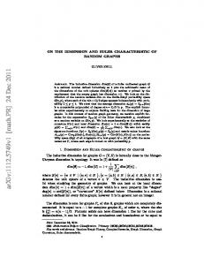
Differential microwave radiometers on the COBE satellite produced the differences in antennae temperature given in Figure 1 at 53 GHz, after removing the dipole radiation due to the motion of the observer relative to the background. The image comprises 6144 pixels, formed by projecting a 32×32 lattice of pixels from each face of a cube onto a sphere. The axes of the cube are alligned with the poles of the ecliptic, and Galactic lattitude and longitude are marked on Figure 1. The value at each pixel is the average of approximately 30,000 individual measurements, and as a first approximation, all pixel values were treated as independent Gaussian random variables although there is a very slight dependence due to antennae beam overlap. The main feature in Figure 1 is radiation from our own Galaxy, visible as a sinusoidal patch across the centre of the image. The Reduced Galaxy (RG) map takes a linear combination of 31.5, 53 and 90 GHz maps to reduce emission from our Galaxy. This map, smoothed by a FWHM= 7o Gaussian kernel defined below, appears on the cover of the July 1992 issue of Scientific American. Figure 2 shows the smoothed RG map divided by its standard deviation obtained by appropriately smoothing the variance of the approximately 30,000 measurements at each pixel. We are interested in detecting evidence of a signal in this random field, X(t), defined on the unit 2-sphere S.

5.2

Analysis

Under the null hypothesis of no signal, X(t) is an isotropic white noise random field convolved with a Gaussian kernel or ‘point response function’ proportional to exp(−λ||h||2 ), h ∈ IR2 . Thus X(t) is a Gaussian random field with the Gaussian correlation function R(h) = exp(−λ||h||2 /2). It can be shown that such a field then satisfies the conditions of Theorem 1. The width of the kernel is usually measured in terms of its ‘full width at half maximum’, FWHM, or the width of the kernel at half its maximum value, so that ˙ 1/2 = λ, so that comλ = 4 loge 2/FWHM2 . It is straightforward to show that det[Var(X)] bining (4.9), (3.4) and Theorem 3 we get Z ∞ 2 2 1/2 exp(−z 2 /2)/(2π)1/2 dz. (5.1) E[χ(Ax )] = (8 loge 2/FWHM )x exp(−x /2)/(2π) +2 x

This same result (5.1) was also given by Gott et al. (1990). Some excursion sets Ax of X(t) are shown in Figure 3. Their Euler characteristics were approximated by V − E + F , where V is the number of vertices of the pixel grid inside Ax , E is the number of edges, and F is the number of faces. Adler (1977) shows that this converges to χ(Ax ) with probability one as the pixel size tends to zero. A plot of the Euler characteristic against the threshold x is shown in Figure 4, together with the expectation for no signal (5.1). For comparison, the same methods were applied to three independent null data sets obtained by taking the difference of readings from the A and B radiometers at 31.5, 53 and 90 GHz. These data, which should contain no signal, were treated in the same way and added to Figure 4. 11

We could try applying these methods to the reversed field −X(t). However a moment’s reflection will show that there is nothing to be gained; χ(Ax ) for −X(t) almost surely equals two minus χ(A−x ) for X(t), since the boundary of Ax is, with probability one, a union of unconnected closed loops with Euler characteristic equal to zero.

5.3

Discussion

The conclusions are that the three null data sets appear to fit the theoretical expectation quite well, but the RG map which contains the signal shows some discrepancies. There appears to be evidence for an excess number, 6, of connected components in the upper tail (Figure 5a) at about the x = 3.5 level, where we expect only 1.14 if no signal is present. The excursion set for this level is shown in Figure 3. Two of the components lie near the Galactic plane and should be discounted, but the other four lie off the Galactic plane and may represent evidence of true anomolies. At the lower tail shown in Figure 5b the two connected components of low intensity at x = −3.5 are both in the Galactic plane, also marked on Figure 3. The other main features are a reduced Euler characteristic near x = ±1, also shown on Figure 3; here the excursion sets have too few connected components, indicating large regions of higher intensity where x = +1 and large regions of lower intensity where x = −1. However, as Charles L. Bennett of the Goddard Space Flight Center is quoted as saying: “I can’t emphasize strongly enough that you cannot look at any one point and say, ‘That’s a cosmic fluctuation’ ” (Scientific American, July 1992, page 18). A model with a small number of isolated cosmic fluctuations, such as that predicted by cosmic strings or texture (see Torres, 1994), would give quite a different Euler characteristic plot. Worsley et al. (1993) showed that a small number of isolated peaks in the signal component of X(t) increased the Euler characteristic well above its null expectation for large thresholds x, while the rest of the plot showed reasonable agreement between observed and expected Euler characteristic. The fact that Figure 4 does not look like this contributes evidence against the cosmic strings and texture hypotheses. A simple explanation for the observed discrepancies in the Euler characteristic can be found as follows. Note that the unsmoothed data is very nearly white noise, to which some signal is added. Suppose we model this signal as a realisation of yet another smooth Gaussian random field. The smoothed data X(t) can then be modelled as the sum of a FWHM= 7o zero mean unit variance noise component with plus a smoothed signal component which is a realisation of a FWHM= W zero mean Gaussian random field with variance σ 2 , say. The values of σ 2 and W were estimated by equating the variance of X and the variance of its ˙ to their sample values, to give σ ˆ = 25o . The expectation of the derivative X ˆ 2 = 0.6 and W Euler characteristic for this field, taken over all realisations of the signal as well as the noise, behaves like that of a zero mean 1.6 variance Gaussian random field with effective full width at half maximum equal to 8.65o . The expected Euler characteristic for this has been added to Figure 4 and it appears to be reasonably close to the observed values. This explanation is in agreement with the inflation hypothesis for the big-bang model (Torres, 1994). These calculations are only used to illustrate the theory and several possibly important features of the data have not been taken into account. Systematic effects due to the small kinematic quadrupole have not been removed, and the analysis could be contaminated by the uncertain contributions from the Galaxy not fully removed in the RG map. The analysis 12

also ignores second order effects caused by the slight correlation between adjacent pixels in the unsmoothed data, and the correlation induced by removing the monopole and dipole radiation. However the broad conclusion is similar to that reported by Torres (1994) who also found that the Euler characteristic agreed with that expected from a zero mean Gaussian random field.

References Adler, R.J. (1977). A spectral moment estimator in two dimensions. Biometrika, 64, 367-373. Adler, R.J. (1981). The Geometry of Random Fields. Wiley, New York. Flanders, H. (1963). Differential forms with applications to the physical sciences. Academic Press, New York. Gott, J.R., Melott, A.L. and Dickinson, M. (1986). The sponge-like topology of large scale structures in the universe. Astrophysical Journal, 306, 341-357. Gott, J.R., Park, C., Juskiewicz, R., Bies, W.E., Bennett, D.P., Bouchet, F.R. and Stebbins, A. (1990). Topology of microwave background fluctuations: theory. Astrophysical Journal, 352, 1-14. Hadwiger, H. (1959). Normale K¨orper im euklidischen Raum und ihre topologischen und metrischen Eigenschaften. Mathematische Zeitschrift, 71, 124-140. Kent, J.T. (1989). Continuity properties for random fields. The Annals of Probability, 17, 1432-1440. Knuth, D.E. (1992). Two notes on notation. The American Mathematical Monthly, 99, 403-422. Morse, M. and Cairns, S.S. (1969). Critical Point Theory in Global Analysis and Differential Topology. Academic Press, New York. Rhoads, J.E., Gott, J.R. and Postman, M. (1994). The genus curve of the Abell clusters. Astrophysical Journal, 421, 1-8. Siegmund, D.O and Worsley, K.J. (1995). Testing for a signal with unknown location and scale in a stationary Gaussian random field. Annals of Statistics, /bf 23, 608-639. Smoot, G.F., Bennett, C.L., Kogut, A., Wright, E.L., Aymon, J., Boggess, N.W., Cheng, E.S., De Amici, G., Gulkis, S., Hauser, M.G., Hinshaw, G., Jackson, P.D., Janssen, M., Kaita, E., Kelsall, T., Keegstra, P., Lineweaver, C., Lowenstein, K., Lubin, P., Mather, J., Meyer, S.S., Moseley, S.H., Murdock, T., Rokke, L., Silverberg, R.F., Tenorio, L., Weiss, R. and Wilkinson, D.T. (1992). Structure in the COBE differential microwave radiometer first-year maps. Astrophysical Journal, 396, L1-L5. 13

Torres, S. (1994). Topological analysis of COBE-DMR cosmic microwave background maps. Astrophysical Journal, 423, L9-L12. Worsley, K.J. (1995). Estimating the number of peaks in a random field using the Hadwiger characteristic of excursion sets, with applications to medical images. Annals of Statistics, 23, 640-669. Worsley, K.J. (1994). Local maxima and the expected Euler characteristic of excursion sets of χ2 , F and t fields. Advances in Applied Probability, 26, 13-42. Worsley, K.J., Evans, A.C., Marrett, S. and Neelin, P. (1992). A three dimensional statistical analysis for CBF activation studies in human brain. Journal of Cerebral Blood Flow and Metabolism, 12, 900-918. Worsley, K.J., Evans, A.C., Marrett, S. and Neelin, P. (1993). Detecting changes in random fields and applications to medical images. Journal of the American Statistical Association, submitted for publication.

14

Figure 1. 53 GHz map, dipole removed, no smoothing 60

330 60 0

330 240 270 300 330 210 180 210

30

Galactic centre

240

30

180

30 330

0

60

150 -30

0

-30 30

180 330 300 240 210 0270 30 150

-30 150

120 90

180

-60 -60 60-6090 120 150

60 -0.5

0

0.5

1

x 10^-3 Kelvin

15

1.5

Figure 2. X(t) = standardized Reduced Galaxy (RG) map, 7 degree smoothing

Galactic centre

-4

-2

0

X(t)

16

2

4

Figure 3: Excursion sets of X(t)

Galactic centre

-3.5

-1

X(t)

17

1

3.5

0 -50

Euler characteristic

50

Figure 4. Euler characteristic of excursion sets of X(t)

Reduced Galaxy (RG) (A-B)/2, no signal expected, no signal fitted to RG

-4

-2

0 threshold, x

18

2

4

8 6 4 2 0

Euler characteristic

10

Figure 5a. Euler characteristic, upper tail

3.0

3.5

4.0

4.5

threshold, x

0 -2 -6

-4

Reduced Galaxy (RG) (A-B)/2, no signal expected, no signal fitted to RG

-8

Euler characteristic

2

Figure 5b. Euler characteristic, lower tail

-4.5

-4.0

-3.5 threshold, x

19

-3.0