arXiv:1706.02567v2 [cond-mat.stat-mech] 16 Aug 2017
Boundary Effects on Population Dynamics in Stochastic Lattice Lotka–Volterra Models Bassel Heiba, Sheng Chen, and Uwe C. T¨auber Department of Physics (MC 0435) and Center for Soft Matter and Biological Physics, Robeson Hall, 850 West Campus Drive, Virginia Tech, Blacksburg, Virginia 24061, USA
Abstract We investigate spatially inhomogeneous versions of the stochastic Lotka–Volterra model for predator-prey competition and coexistence by means of Monte Carlo simulations on a two-dimensional lattice with periodic boundary conditions. To study boundary effects for this paradigmatic population dynamics system, we employ a simulation domain split into two patches: Upon setting the predation rates at two distinct values, one half of the system resides in an absorbing state where only the prey survives, while the other half attains a stable coexistence state wherein both species remain active. At the domain boundary, we observe a marked enhancement of the predator population density. The predator correlation length displays a minimum at the boundary, before reaching its asymptotic constant value deep in the active region. The frequency of the population oscillations appears only very weakly affected by the existence of two distinct domains, in contrast to their attenuation rate, which assumes its largest value there. We also observe that boundary effects become less prominent as the system is successively divided into subdomains in a checkerboard pattern, with two different reaction rates assigned to neighboring patches. When the domain size becomes reduced to the scale of the correlation length, the mean population densities attain values that are very similar to those in a disordered system with randomly assigned reaction rates drawn from a bimodal distribution.
Email address:
[email protected],
[email protected],
[email protected] (Bassel Heiba, Sheng Chen, and Uwe C. T¨ auber)
Preprint submitted to Physica A
August 17, 2017
Keywords: stochastic population dynamics, Lotka–Volterra predator-prey competition, spatial inhomogeneities, boundary effects, quenched disorder
1. Introduction Due to its wide range of applications and relative simplicity, variants of the Lotka–Volterra predator-prey competition model represent paradigmatic systems to study the emergence of biodiversity in ecology, noise-induced pattern formation in population dynamics and (bio-)chemical reactions, and phase transitions in far-from-equilibrium systems. In the classical deterministic Lotka– Volterra model [1, 2], two coupled mean-field rate equations describe the population dynamics of a two-species predator-prey system, whose solutions display periodic non-linear oscillations fully determined by the system’s initial state. Yet the original mean-field Lotka–Volterra rate equations do not incorporate demographic fluctuations and internal noise induced by the stochastic reproduction and predation reactions in coupled ecosystems encountered in nature. In a series of analytical [3]–[6] and numerical simulation studies [7]–[18], the population dynamics of several stochastic spatially extended lattice Lotka–Volterra model variants was found to substantially differ from the mean-field rate equation predictions due to stochasticity and the emergence of strong spatio-temporal correlations: Both predator and prey populations oscillate erratically, and do not return to their initial densities; the oscillations are moreover damped and asymptotically reach a quasi-stationary state with both population densities finite and constant on one- or two-dimensional square lattices [7], whereas damping appears absent or is very weak in three dimensions [9]. Very similar dynamical properties are observed in other two-dimensional model variants, including a predator-prey system with added prey food supply and cover [12], and implementations on a triangular lattice [14]. In a non-spatial setting, the persistent non-linear oscillations can be understood through resonantly amplified demographic fluctuations [19]. Local carrying capacity restrictions, representing limited resources in nature, can be implemented in lattice simulations by con-
2
straining the number of particles on each site [8, 10, 11, 15, 16, 17]. These local occupation number restrictions cause the emergence of a predator extinction threshold and an absorbing phase, wherein the predator species ultimately disappears while the prey proliferate through the entire system. Upon tuning the reaction rates, one thus encounters a continuous active-to-absorbing state nonequilibrium phase transition whose universal features turn out to be governed by the directed percolation universality class [4, 5, 10, 11, 12, 15, 16, 18]. Biologically more relevant models should include spatial rate variability to account for environmental disorder. The population dynamics in a patch surrounded by a hostile foe [20, 21, 22] is well represented by Fisher’s model [23], which includes diffusive spreading as well as a reaction term capturing interactions between individuals and with the environment. For the stochastic Lotka– Volterra model, the influence of environmental rate variability on the population densities, transient oscillations, spatial correlations, and invasion fronts was investigated by assigning random reaction rates to different lattice sites [24, 25]. Spatial variability in the predation rate results in more localized activity patches, a remarkable increase in the asymptotic population densities, and accelerated front propagation. These studies assumed full environmental disorder, as there was no correlation at all between the reaction rates on neighboring sites. In a more realistic setting, the system should consist of several domains with the environment fairly uniform within each patch, but differing markedly between the domains, e.g., representing different topographies or vegetation states. In our simulations, we split the system into several patches and assign different reaction rates to neighboring regions. By tuning the rate parameters, we can force some domains to be in an absorbing state, where the predators go extinct, or alternatively in an active state for which both species coexist at non-zero densities. One would expect the influence of the boundary between the active and absorbing regions to only extend over a distance on the scale of the characteristic correlation length in the system. In this work, we study the local population densities, correlation length, as well as the local oscillation frequency and attenuation, as functions of the distance from the domain boundary. As we 3
successively divide the system further in a checkerboard pattern so that each patch decreases in size, the population dynamics features quantitatively tend towards those of a randomly disordered model with reaction rates assigned to the lattice sites from a bimodal distribution.
2. Model Description and Background The deterministic classical Lotka–Volterra model [1, 2] is a set of two coupled non-linear dynamical rate equations that on a mean-field approximation level capture the following kinetic reactions of two species, respectively identified with predators A and prey B: µ
A → ∅,
λ
A + B → A + A,
σ
B →B+B.
(1)
In these stochastic processes, µ corresponds to the spontaneous predator death rate, while σ denotes the prey reproduction rate. Finally, λ is the predation rate which describes the non-linear reaction through which the predator and prey species interact with each other. The simplified Lotka–Volterra model thus assumes that the prey population grows exponentially in the absence of predators, but becomes diminished with growing predator population. In the presence of the prey, the predator population will increase with the prey population, but is subject to exponential decay once all prey are gone. The configuration with vanishing predator number represents an absorbing state for this system, since there exists no stochastic reaction process that would allow recovery from it. For completeness, we mention that the total population extinction state of course represents another absorbing state. We also remark that one could add independent predator reproduction A → A + A (with rate σ 0 ) and prey death B → ∅ (rate µ0 ) processes to the standard Lotka–Volterra kinetics (1). Yet this would induce no qualitative changes as long as σ 0 < µ and σ > µ0 ; one then simply needs to replace µ with the rate difference µ − σ 0 , and σ with σ − µ0 . The associated rate equations, subject to mean-field mass action factorization for the non-linear predation process, and valid under well-mixed conditions
4
for spatially homogeneous time-dependent particle densities a(t) and b(t), read ˙ = −λ0 a(t)b(t) + σ 0 b(t) , b(t)
a(t) ˙ = λ0 a(t)b(t) − µ0 a(t) ,
(2)
with continuum reaction rates λ0 , µ0 , and σ 0 . Since there exists a conserved first integral (Lyapunov function) K = λ0 (a + b) − σ 0 ln a − µ0 ln b = const. for this deterministic dynamics, the solutions to eqs. (2) are strictly periodic nonlinear oscillations that precisely return to the system’s initial state. Although popular in the fields of ecology and biology, the Lotka–Volterra model is also often criticized for being too simplistic and mathematically unstable. This is due to several simplifying and likely unrealistic assumptions: First, the prey always have a sufficient amount of food available, whence its depletion is neglected, and the prey’s nourishment source is not explicitly represented in the model. Second, the only source of food for the predator species is the prey, and its consumption is a necessary requirement for the predators’ reproduction. Third, there is no specified limit on the prey intake for the predators. Fourth, the rate of change of either population is directly proportional to its size. Finally, during the temporal evolution any environmental influence is assumed fixed in time, and crucial concepts such as trait inheritance, mutations, or natural selection play no role. In our research, we use Monte Carlo simulations for the stochastic Lotka– Volterra model based on the reactions (1) performed on a two-dimensional square lattice with 512 × 512 sites and periodic boundary conditions to fully account for emerging spatial structures and internal reaction noise. We note that we have also performed simulations on two-dimensional square lattices with 256 × 256 and 128 × 128 sites; aside from overall noisier data, as one would expect, we obtain no noticeable quantitative differences. Given that the correlation lengths ξ measured below are much smaller than these system sizes, this is not surprising. Due to our limited computational resources, we have not attempted runs on even larger systems. In the following, all listed Monte Carlo data and extracted quantitative results refer to 512 × 512 square lattices. Also, for the reaction processes, we only consider the four nearest-neighbor sites, and 5
have not extended interactions to larger distances. In our model, we implement occupation number limitations or finite local carrying capacities; i.e., the number of particles on any lattice site is restricted to be either 0, if the site is empty, or 1, if it is occupied by a predator or a prey individual. We shall examine the population densities of each species, given by their total particle number divided by the number of lattice sites, and aim to quantify the ensuing oscillations and through characteristic observables that include their frequency and attenuation, as well as typical population cluster sizes as determined by their spatial correlation length. The simulation algorithm for the death, reproduction, and mutual interactions of the prey and predator particles proceeds as follows [26, 7, 9]: For each iteration, an occupied site is randomly selected and then one of its four adjacent sites is picked at random. If the two selected sites contain a predator and a prey particle, a random number x1 ∈ [0, 1] is generated; if x1 < λ, the prey individual is removed and a newly generated predator takes its place. Similarly, if the occupant is a predator, a random number x2 ∈ [0, 1] is generated, and the particle is removed if x2 < µ. Yet if the initially selected occupant is a prey particle and the chosen neighbor site empty, a random number x3 ∈ [0, 1] is generated; if x3 < σ a new prey individual is added to this site. One Monte Carlo Step (MCS) is considered completed when on average all particles have participated in the reactions once. The variables that can be tuned in our simulations are: the system size L, the initial predator density ρA (0), the initial prey density ρB (0), the predator death rate µ, the prey reproduction rate σ, the predation rate λ, and the number of Monte Carlo steps. We chose the linear system size L = 512. Naturally one must avoid starting the simulations from one of the absorbing states. For any non-zero initial predator and prey density, the population numbers and particle distribution at the outset of the simulation runs influence the system merely for a limited time, and the final (quasi-)stationary state of the system is only determined by the three reaction rates [18]. In our simulations, the rates µ and σ are kept constant for simplicity, while λ is considered to be the only relevant 6
1.0
λ =0.1 λ =0.18 λ =0.4
0.9 0.8
ρB (t)
0.7 0.6 0.5 0.4 0.3 0.2 0.1 0.0
0.1
0.2
ρA (t)
0.3
0.4
0.5
Figure 1: Monte Carlo simulation trajectories for a stochastic Lotka–Volterra model on a 512×512 square lattice with periodic boundary conditions and restricted site occupancy shown in the predator ρA (t) versus prey density ρB (t) phase plane (ρA (t) + ρB (t) ≤ 1) with initial values ρA (0) = 0.3 = ρB (0), fixed reaction probabilities µ = 0.125, σ = 1.0, and different predation efficiencies: (i) λ = 0.1 (black dots): predator extinction phase; (ii) λ = 0.18 (green stars): direct exponential relaxation to the quasi-stationary state just above the extinction threshold in the predator-prey coexistence phase; (iii) λ = 0.4 (red triangles): the trajectory spirals into a stable fixed point, signifying damped oscillations deep in the coexistence phase.
control parameter. The dynamical properties are generically determined by the ratio of the reaction rates; the subsequent results apply also for different sets of µ and σ with appropriately altered predation rate λ. Since we only have two species, predators and prey, 0 ≤ ρA + ρB ≤ 1 due to the site occupation resctrictions. For each parameter set we use a suitable number of independent simulation runs and use the average of these repeats in the data analysis to reduce statistical errors. In the case of very low predation rates λ, the predators will gradually starve to death, and the remaining prey will finally occupy the whole system. On the other hand, when λ is large, there is a finite probability (in any finite lattice) that all prey individuals would be devoured; subsequently the predators would die out as well because of starvation. In fact, the absorbing extinction state is the only truly stable state in a finite population with the stochastic dynamics (1).
7
However, in sufficiently large systems, quasi-stable states in which both species survive with relatively constant population densities during the entire simulation duration are indeed observed in certain regions of parameter space. Fig. 1 shows three single-run simulation results, plotting the prey population density ρB (t) versus that of the predators ρA (t) with the reaction probabilities µ = 0.125 and σ = 1.0 held fixed; we thus select the non-linear predation reaction rate λ as the only control parameter. We chose the initial population densities as ρA (0) = 0.3 = ρB (0) with the particles randomly distributed among the lattice sites. With λ = 0.1 (black dots), the predators have low predation efficiency and thus gradually go extinct; the system then reaches an absorbing state with only prey particles remaining and ultimately filling the entire lattice (ρB → 1). If we increase the value of λ to 0.18 (green stars), just above the predator extinction threshold, the system relaxes exponentially to a quasi-stationary state with non-zero densities for both species. For λ = 0.4 (red triangles), the system resides deep in this coexistence phase and the simulation trajectory spirals into a stable fixed point, indicating damped oscillatory kinetics. According to our investigations, we estimate the critical predation rate of the predator extinction phase transition point at λc = 0.12 ± 0.01.
3. Boundary Effects at a Coexistence / Predator Extinction Interface Natural environments vary in space and boundaries are formed between different regions, yielding often quite sharp interfaces, e.g., between river and land, desert and forest, etc. At the boundaries of such spatially inhomogeneous systems, interesting phenomena may arise. In order to study boundary effects on simple predator-prey population dynamics, we split our simulation domain into two equally large pieces with one half residing in the predator extinction state, and the other half in the two-species coexistence phase. We use a twodimensional lattice with 512 × 512 sites with periodic boundary conditions, and index the columns with integers in the interval [0, 511]. Whereas the predator death and prey reproducation rates are uniformly set as µ = 0.125 and σ = 1.0
8
(a)
(b)
(c)
Figure 2: Snapshots of the spatial particle distribution on a 512 × 512 lattice (with periodic boundary conditions) that is split into equally large predator extinction (left) and species coexistence (right) regions: prey are indicated in green, predators in red, white spaces in white. (a) Random initial distribution with densities ρA = 0.3 = ρB ; (b) state of the system after 1000 MCS, when it has reached a quasi-stationary state with uniform rates µ = 0.125 and σ = 1.0, while λl = 0.1 on columns [0, 255], λr = 0.8 on columns [256, 511]; (c) close-up of a local 100 × 50 area at the boundary.
on all sites, we assign λl = 0.1 < λc on columns [0, 255] to enforce predator extinction on the “left” side, and λr = 0.8 > λc for the columns on the “right” half with indices [256, 511], which is thus held in the predator-prey coexistence state. Fig. 2(a) depicts the initial random particle distribution with equal population densities ρA = 0.3 = ρB . After the system has evolved for 1000 MCS, a quasi-steady state is obtained as shown in Fig. 2(b), and the close-up near the boundary (c). The predators are able to penetrate into the “left” absorbing region by less than 10 columns, and no predator individuals are encountered far away from the active-absorbing interface. On the right half, we observe a predator-prey coexistence state with the prey particles forming clusters surrounded by predators and predation reactions occurring at their perimeters. Since only the predator species is subject to the extinction transition into an absorbing state, while the prey can survive throughout the entire simulation domain, we concentrate on boundary effects affecting the predator population. We measure the column densities of predators ρA (n), defined as the number of
9
predators on column n divided by L = 512, and record their averages from 1000 independent simulation runs as a function of column index n. As shown in the inset of Fig. 3(a), ρA (n) decreases to 0 deep inside the absorbing half of the system, and reaches a positive constant 0.195 ± 0.001 within the active region. The main graph focuses on the boundary region, where we observe a marked predator density peak right at the interface (column 256). The predator density enhancement at the boundary is obviously due to the net intrusion flow of species A from the active subdomain with high predation rate into the predator extinction region with abundant food in the form of the near uniformly spread prey population. We also ran simulations for other predation rate pairs such as λl = 0.1 and λr = 0.2 (still in the coexistence phase), and observed very similar behavior (except that the peak of ρA appeared on column 257 in that situation instead of at n = 256). Fig. 3(b) shows the exponential decay of the predator column density ρA (n) as function of the distance |255 − n| from the boundary (located at n = 255) towards the “left”, absorbing side. A simple linear regression gives the inverse characteristic decay length k = −0.286. However, on the “right” active half of the system, ρA (n) neither fits exponential nor algebraic decay. Instead, ρA reaches the asymptotic constant value 0.195 ± 0.001 deep in the coexistence l
region through an apparent stretched exponential form ρA (n) ∼ e−(n−256) + 0.195 with stretching exponent l ≈ 0.348, as demonstrated in Fig. 3(c). On the “right” semidomain set in the predator-prey coexistence phase, the particle reproduction processes induce clustering of individuals from each species. The cluster size may vary with the distance from the boundary.
We uti-
lize the correlation length ξ, obtained from the equal-time correlation function C(x), to characterize the spatial extent of these clusters. For species α, β = A, B, the (connected) correlation functions are defined as Cαβ (x) = hnα (x) nβ (0)i−hnα (x)i hnβ (0)i, where nα (x) = 0, 1 denotes the local occupation number of species α at site x [17]. For x = 0 and α = β, in a spatially homogeneous system it is simply given by the density hnA i: Cαα (0) = hnA i(1 − hnA i). For |x| > 0, hnα (x) nβ (0)i is computed as follows: First choose a site, and then 10
1 (b)
(a)
2
0.7
3
300
n
ρA
0.6
0.8 (c)
log10(−ln(ρA −0.195))
0.6 0.5 0.4 0.8 0.3 0.2 0.1 0.0 0
ln(ρA )
1.0
0.4
0.6
4 5
0.5
6 0.2 0.0 250
0.4
7 260
n
270
80 5 10 15 20
255-n
0.30.0 0.4 0.8 1.2
log10(n−256)
Figure 3: After the split system with rates µ = 0.125, σ = 1.0 and λl = 0.1 on columns [0, 255], λr = 0.8 on columns [256, 511] evolves for 1000 MCS, it arrives at a quasi-stationary state: (a) the main plot shows the column densities of the predator population ρA (n) as function of column index n ∈ [251, 270] with the error bars indicating the standard deviation, and the inset on all L = 512 columns (data averaged over 1000 independent runs); (b) exponential decay of ρA (n) from the boundary (located at n = 255) into the absorbing region with n ∈ [235, 255]: The blue dots depict our simulation results, while the black straight line represents a linear regression of the data with slope k = −0.286; (c) the column density ρA decays to a positive constant value 0.195 ± 0.001 deep in the right coexistence region. The blue dots display log10 (− ln(ρA − 0.195)) versus log10 (n − 256), while the black straight line with slope l = 0.348 is obtained from linear data regression.
a second site at distance x away from the first one. nα (x) nβ (0) equals 1 only if the first site is occupied by an individual of species β, and the second one by an particle of species α, otherwise the result is 0. One then averages over all sites. Here, we compute the predator correlations CAA (x, n) on a given column n, i.e., we only take the mean in the above procedure over the L = 512 sites on that column. The main panel in Fig. 4(a) shows the predator correlation function CAA (x) on column n = 274 with x ∈ [0, 9], where the CAA (x) gradually decreases to zero. The inset presents the same data in a logarithmic scale, demonstrating exponential decay according to C(x, n) ∼ e−x/ξ(n) . Since the statistical errors grow at large distances x, we only use the initial data points up to x = 6 for the analysis. Linear regression of ln(CAA (x, n = 274)) over
11
0.10
1 2 3 4 5 6 7 8 0 2 4 6 8 10
2.5
x
0.05
2.0 1.5
0.00 0.05 0
(b)
3.0
ξ
0.15
C(x)
3.5
(a)
ln(C(x))
0.20
1.0 2
4
x
6
8
10
0.5 255 260 265 270 275
n
Figure 4: (a) Main panel: the predator correlation function CAA (x, n) on column n = 274 (data averaged over 1000 independent simulation runs). Inset: ln(CAA (x, n)); the red straight line indicates a simple linear regression of the data points with x ∈ [1, 6], and yields the characteristic decay length ξ(n = 274) ≈ 3.2; the error bars indicate the standard deviation. (b) Correlation length ξ(n) versus column number n, with ξ(n) defined as the negative reciprocal of the slope of ln(CAA (x, n)).
x ∈ [1, 6] gives ξ(n = 274) ≈ 3.2, indicated as red square in Fig. 4(b). In the same manner, we obtain the characteristic correlation lengths ξ(n) for each column n as shown in Fig. 4(b), starting at the interface at n = 256. We observe ξ(n) to increase by about a factor of four within the first ten columns away from the boundary, and then saturate at the bulk value ξ ≈ 3.2. Near the absorbing region, the predator clusters are thus much smaller, owing to the net flux of predators across the boundary into the extinction domain. These values of ξ are measured after the entire system has reached its (quasi-)steady state after 1000 MCS, and would not change for longer simulations run times. We note that the relationship between the correlation length ξ and the predation rate λ is manifestly not linear, i.e., a very large value of λ does not imply huge predator clusters. We surmise that the cluster size remains finite even in that scenario, and the predators would penetrate into the “left” absorbing region for a finite number of columns only. For sufficiently large domain size, the system should thus remain spatially inhomogeneous even for very high predation rates
12
0.6 0.5
ρA (t)
0.4
column 256 column 274
0.3 0.2 0.1 0.00
20
40
60
80 100 120 140 160
t [MCS]
Figure 5: The temporal evolution of the average predator column densities ρA (t, n) (averaged over 1000 independent runs) on columns n = 256 (blue dots) and n = 274 (red plus marks), with initial predator density ρA (0) = 0.3 and rates µ = 0.125, σ = 1.0, λl = 0.1 on columns n ∈ [0, 255], and λr = 0.8 for n ∈ [256, 511].
λ. Finally, the dependence of the typical cluster size ξ(n) on column index n correlates inversely with the column density plotted in Fig. 3: High local density corresponds to small cluster size and vice versa. We note that the product ρA (n) ξ(n) is however not simply constant across different columns; rather it is minimal near the boundary (at n = 256), then increases away from the interface, and ultimately reaches a fixed value within 10 columns inside the active region. Spatially homogeneous stochastic Lotka–Volterra systems display damped population oscillations in the predator-prey coexistence phase after being initialized with random species distribution, see, for example, the (red triangle) trajectory in Fig. 1 for predation rate λ = 0.4. We next explore the boundary effects on these population oscillations near the active-absorbing interface. We prepare the system with the same parameters as mentioned above so that its “left” half is in the absorbing state while the “right” side sustains species coexistence. The initial population densities are again set to ρA (0) = 0.3 = ρB (0), with the particles randomly distributed on the lattice. We then measure the column predator densities as a function of time (MCS). Fig. 5 displays the temporal evolution of ρA (t, n) on columns n = 256 and n = 274. We observe the oscil-
13
0.014 (a) 0.012 0.010
11 9 8
0.008 0.006
7 6
0.004
5
0.002 0.000 0.000
(b)
10
tc
f(ω)
12
256 258 262 266 270 274
4 0.628
−1
ω[MCS ]
1.256
3256 264 272 280 288
n
Figure 6: (a) Fourier transform amplitude fA (ω, n) of the predator column density time evolution on columns n = 256 (blue dots), 258 (green triangles up), 262 (red triangles down), 266 (cyan squares), 270 (magenta stars), and 274 (black plus marks), with rates µ = 0.125, σ = 1.0, and λl = 0.1 for n ∈ [0, 255], λr = 0.8 for n ∈ [256, 511]; (b) measured characteristic decay time tc (n) on columns near the active-absorbing boundary, inferred from the peak widths in (a), with the error bars representing the standard deviation.
lations on the column closest to the interface to be strongly damped, whereas deeper inside the active region the population oscillations are more persistent and subject to much weaker attenuation. Both column densities asymptotically reach the expected quasi-steady state values. In order to determine the dependence of the local oscillation frequencies on the distance from the active-absorbing interface, we compute the Fourier R transform amplitude fA (ω, n) = | e−iωt ρA (t, n) dt| of the column density time series data by means of the fast Fourier transform algorithm for n ∈ [256, 274], as shown in Fig. 6(a). Assuming the approximate functional form ρA (t, n) ∼ e−t/tc (n) cos(2πt/T (n)), we may then identify the peak position of fA (ω, n) with the characteristic oscillation frequency 2π/T (n), and the peak half-width at half maximum with the attenuation rate or inverse relaxation time 1/tc (n). We find that the oscillation frequencies are constant except for the column at the boundary (n = 256), which shows a very slight enhancement. We conclude that the presence of the extinction region does not markedly affect the frequency
14
(a)
(b)
(c)
Figure 7: Snapshots of the distribution of predator (red) and prey (green) particles after the system has evolved for 1000 MCS with rates µ = 0.125, σ = 1.0, and λ switched alternatingly between the values 0.1 (predator extinction) and 0.8 (species coexistence) on neighboring subdomains, as the full 512 × 512 system is periodically divided into successively smaller square patches with lengths 256 (a), 64 (b), and 16 (c), respectively. The square subdomains dominantly colored in green reside in the extinction state (λ = 0.1), whereas predator-prey coexistence pertains to the other patches (λ = 0.8).
of the population oscillations in the active regime. In contrast, the attenuation rate increases by a factor of three within about 20 columns in the vicinity of the interface, as demonstrated in Fig. 6(b). Beyond n ≈ 278 in the coexistence region, the relaxation time assumes its constant bulk value.
4. Checkerboard Division of the System To further explore boundary (and finite-size) effects in spatially inhomogeneous Lotka–Volterra systems, we proceed by successively dividing the simulation domain into subdomains in a checkerboard pattern, setting the predation rate to two distinct values in neighboring patches, and thus preparing them alternatingly in either the active coexistence or absorbing predator extinction states. Fig. 7(a) shows a case when the system is split into four subregions with σ = 1.0 and µ = 0.125, and with two distinct values for the predation rate λ = 0.1 and 0.8 assigned to alternating patches of the 2 × 2 checkerboard structure. Note that the low predation rate value posits the corresponding patches in the predator extinction state, whereas the subdomains with the high predation
15
rate reside in the species coexistence phase. Figures 7(b) and (c) depict the situations when the total simulation domain with 512 × 512 sites is respectively split into 8 × 8 and 32 × 32 square patches: If for a given box λ is set to 0.1, then the adjacent square subdomains above, below, to its right, and to its left are given a value λ = 0.8. 1000 simulations were performed for each setting, and the averages over these independent runs were used to analyze the data. We also generated and inspected simulation videos: snapshots are depicted in Fig. 7. As we split the system into successively smaller and more pieces in the checkerboard-patterned fashion with λ switching between 0.1 and 0.8 on neighboring subregions, we find the boundaries to have less of an impact on the population densities. We observe that in this sequence the prey density decreases on the patches with lower predation rate 0.1, but stays roughly the same on the subdomains where λ = 0.8. The predator density in contrast increases in both the active and absorbing regions as the subdivision proceeds. We have also confirmed that these changes in the total population densities naturally become less significant if the two different predation rate values are chosen closer to each other. In Fig. 8, we plot the total (summed over all subdomains) predator and prey population densities ρ in the simulation domain split into N × N checkerboard patches, as functions of log10 N . Here, N = 1 corresponds to the situation studied in section 3, where the system was divided into two rectangular subdomains. The other values of N = 512, 256, 128, 64, 32, 16, 8, 2 refer to checkerboard square patches with lengths 512/N . The mean population density ρ shown for each data point represents an average of 1000 independent simulation runs; the associated statistical error was very small, with a standard deviation of order 10−3 . As apparent in the data, the overall population predator density ρA monotonically increases with growing number N of subdivisions, while the prey density ρB decreases. We also performed the analogous sequence of measurements for other pairs of predation rate values. For instance, with checkerboard subdomains with λ = 0.1 and 0.2 (also just within the species coexistence range, see Fig. 1), 16
0.6
ρA (N) ρAr ρB (N) ρBr
0.5
ρ
0.4 0.3 0.2 0.1 0 10
101
N
102
103
Figure 8: Total population densities for predators (red triangles) and prey (green squares) versus number of checkerboard-patterned subdivisions N of the simulation domain, after the system has evolved for 1000 MCS and reached a quasi-stationary state, with reaction rates µ = 0.125, σ = 1.0, and λ alternatingly switched between 0.1 and 0.8. For comparison, the graph also shows the total quasi-steady state population densities for predators (black plus) and prey (blue star) in a system with randomly assigned predation, drawn with equal probability from a bimodal distribution with values λ = 0.1 and 0.8.
the population density changes with increasing N are less pronounced than in Fig. 8, and ρA , ρB acquire maximum and minimum values at N = 256 rather than 512. The origin of this slight shift can be traced to the fact that the predator correlation length is of order one lattice constant at the boundary of the λ = 0.1/0.8 system, but extends over about two sites for the 0.1/0.2 case. For comparison, we also measured the overall population predator and prey densities in a Lotka–Volterra system with quenched spatial disorder in the predation rates, where either of the two values λ = 0.1 and 0.8 are assigned at random to each lattice site with equal probability. The resulting net population density values are also shown in Fig. 8; they are close, but not identical to those obtained for the N = 512 system, for which these two predation rates are alternatingly assigned to the lattice sites in a periodic regular manner. We would expect the population densities in these two distinct systems to reach equal values if the associated correlation lengths at the boundaries were large compared to the lattice constant, which is however not the case here. 17
5. Conclusion In this work, we have focused on studying boundary effects in a stochastic Lotka–Volterra predator-prey competition model on a two-dimensional lattice, by means of detailed Monte Carlo simulations. We first considered a system split into two equally large parts with distinct non-linear predation rates, such that one domain is set to be in the predator extinction state, while the other one resides in the two-species coexistence phase. We have primarily addressed the influence of such an absorbing-active separation on both populations’ density oscillations as function of the distance from the boundary. We find a remarkable peak in the column density oscillation amplitude of the predator population, as shown in Fig. 3(a), which reflects its net steady influx towards the absorbing region. Correspondingly, the predator correlation length that characterizes the typical cluster size reaches a minimum value at the boundary, see Fig. 4(b). The population oscillation frequency there shows only small deviations from its bulk value, while the attenuation rate is locally strongly enhanced, see Fig. 6(b), inducing overdamped relaxation kinetics. Overall, the ecosystem remains stable. Furthermore, upon splitting the system successively into more pieces in a checkerboard fashion, the observed boundary effects become less significant, and as demonstrated in Fig. 8, the overall population densities acquire values that are close to those in a disordered system with randomly assigned predation rates drawn from a bimodal distribution.
References References [1] Lotka A J 1920 Undamped oscillations derived from the law of mass action J. Am. Chem. Soc. 42 1595 [2] Volterra V 1926 Fluctuations in the abundance of a species considered mathematically Nature 118 558 18
[3] Matsuda H, Ogita N, Sasaki A and Sat¯o K 1992 Statistical mechanics of population – the lattice Lotka–Volterra model Progr. Theor. Phys. 88 1035 [4] Satulovsky J E and Tom´e T 1994 Stochastic lattice gas model for a predatorprey system Phys. Rev. E 49 5073 [5] Boccara N, Roblin O and Roger M 1994 Automata network predator-prey model with pursuit and evasion Phys. Rev. E 50 4531 [6] Durrett R 1999 Stochastic spatial models SIAM Review 41 677 [7] Provata A, Nicolis G and Baras F 1999 Oscillatory dynamics in lowdimensional supports: a lattice Lotka-Volterra model J. Chem. Phys. 110 8361 [8] Rozenfeld A F and Albano E V 1999 Study of a lattice-gas model for a prey-predator system Physica A 266 322 [9] Lipowski A 1999 Oscillatory behavior in a lattice prey-predator system Phys. Rev. E 60 5179 [10] Lipowski A and Lipowska D 2000 Nonequilibrium phase transition in a lattice prey-predator system Physica A 276 456 [11] Monetti R, Rozenfeld A and Albano E 2000 Study of interacting particle systems: the transition to the oscillatory behavior of a prey-predator model Physica A 283 52 [12] Droz M and P¸ekalski A 2001 Coexistence in a predator-prey system Phys. Rev. E 63 051909 [13] Antal T and Droz M 2001 Phase transitions and oscillations in a lattice prey-predator model Phys. Rev. E 63 056119 [14] Kowalik M, Lipowski A and Ferreira A L 2002 Oscillations and dynamics in a two-dimensional prey-predator system Phys. Rev. E 66 066107
19
[15] Mobilia M, Georgiev I T and T¨auber U C 2006 Fluctuations and correlations in lattice models for predator-prey interaction Phys. Rev. E 73 040903 [16] Mobilia M, Georgiev I T and T¨auber U C 2007 Phase transitions and spatio-temporal fluctuations in stochastic lattice Lotka–Volterra models J. Stat. Phys. 128 447 [17] Washenberger M J, Mobilia M and T¨auber U C 2007 Influence of local carrying capacity restrictions on stochastic predator-prey models J. Phys. Cond. Matt. 19 065139 [18] Chen S and T¨ auber U C 2016 Non-equilibrium relaxation in a stochastic lattice Lotka-Volterra model Phys. Biol. 13 2,3 [19] McKane A J and Newman T J 2005 Predator-prey cycles from resonant amplification of demographic stochasticity Phys. Rev. Lett. 94 218102 [20] Skellam J G 1951 Biometrika 38 196 [21] Dahmen K A, Nelson D R, and Shnerb N M 1999 Population dynamics and non-Hermitian localization Statistical Mechanics of Biocomplexity 527 124 [22] M´endez and Campos D 2008 Population extinction and survival in a hostile environment Phys. Rev. E 77 022901 [23] Fisher R A 1937 Ann. Eugen. 7 335 [24] Dobramysl U and T¨ auber U C 2008 Spatial variability enhances species fitness in stochastic predator-prey interactions Phys. Rev. Lett. 101 258102 [25] Dobramysl U and T¨ auber U C 2013 Environmental versus demographic variability in two-species predator-prey models Phys. Rev. Lett. 110 048105 [26] Ziff R M, Gulari E and Barshad Y 1986 Kinetic Phase Transitions in an Irreversible Surface-Reaction Model Phys. Rev. Lett. 56 2553
20