Boundary handling and adaptive time-stepping for PCISPH. Markus Ihmsen Nadir Akinci Marc Gissler Matthias Teschner. University of Freiburg. Abstract.
Workshop on Virtual Reality Interaction and Physical Simulation VRIPHYS (2010) J. Bender, K. Erleben, and M. Teschner (Editors)
Boundary handling and adaptive time-stepping for PCISPH Markus Ihmsen
Nadir Akinci
Marc Gissler
Matthias Teschner
University of Freiburg
Abstract We present a novel boundary handling scheme for incompressible fluids based on Smoothed Particle Hydrodynamics (SPH). In combination with the predictive-corrective incompressible SPH (PCISPH) method, the boundary handling scheme allows for larger time steps compared to existing solutions. Furthermore, an adaptive time-stepping approach is proposed. The approach automatically estimates appropriate time steps independent of the scenario. Due to its adaptivity, the overall computation time of dynamic scenarios is significantly reduced compared to simulations with constant time steps. Categories and Subject Descriptors (according to ACM CCS): I.3.3 [Computer Graphics]: Three-Dimensional Graphics and Realism—Animation
1. Introduction The efficient animation of fast and turbulent fluids can be successfully realized with a variety of Eulerian [MMS04, TKPR06], Lagrangian [APKG07] and semiLagrangian [FF01, LTKF08] methods. This paper focuses on the simulation of incompressible fluids with large time steps using the Lagrangian Smoothed Particle Hydrodynamics (SPH) method. In SPH approaches, the enforcement of the incompressibility is a challenging problem and there exist different strategies to address this issue. For example, projection schemes - similar to Eulerian methods [EFFM02] are successfully employed for particle based approaches, e. g. [CR99, LKO05, HA07, SBH09]. In these methods, velocities are projected onto a divergence-free space by solving a Poisson equation. Small density fluctuations are enforced. The projection, however, is rather expensive to compute for growing particle numbers. In order to reduce expensive computations, state equations are commonly used in Computer Graphics. These equations relate the density with the pressure, while a stiffness parameter governs the compressibility. For compressible fluids, the gas equation [MCG03] and for weakly compressible SPH (WCSPH), the Tait equation [Mon94, BT07] are employed. In order to achieve small density fluctuations, however, the stiffness has to be chosen rather large. This results in large c The Eurographics Association 2010.
pressure jumps for small density variations, which in turn requires small time steps. Recently, a promising method for incompressible SPH has been proposed by Solenthaler and Pajarola [SP09]. In this approach, incompressibility is enforced by iteratively predicting and correcting the density fluctuation. This predictive-corrective incompressible SPH method (PCISPH) provides very smooth density and pressure distributions, resulting in significantly larger time steps compared to the WCSPH method. Although the computation time per simulation step is larger compared to WCSPH, the overall computation time is much smaller. In PCISPH, the density error is propagated within the fluid until the compression is resolved. For large time steps or huge impacts, however, the generally low number of required iterations can grow. In those cases, a smaller time step with less iterations might be more efficient. The number of required iterations also depends on the boundary handling scheme. Basically, existing schemes apply penalty forces, e. g. [MST∗ 04], or force and position corrections, e. g. [BTT09] and [HKK07]. However, for large time steps, typically used in PCISPH, either stiff penalty forces are required or particle stacking occurs in high density regions. High density fluctuations can occur close to the fluid-boundary interface with a negative influence on the time step.
Ihmsen et al. / Boundary handling and adaptive time-stepping for PCISPH
Figure 1: Wave scene. Gentle wave showering three bears, 1.8 million particles. Overall computation time 19.7 hours for 20 real seconds, ∆tmin = 5.1 · 10−4 , ∆tmax = 2.56 · 10−3 .
Our contribution: In this paper, a predictive-corrective boundary handling method for one way fluid-rigid coupling is presented. In contrast to the direct forcing method of [BTT09], the pressure on the boundary is taken into account. Particle stacking is avoided and thus, high density differences at the boundary. The proposed scheme is applied to the PCISPH method and it is shown that high compressions are resolved more smoothly compared to existing boundary methods. Therefore, larger time steps can be used.
more stable form of the repulsion forces using a scaled version of the cubic spline kernel. But still, the main difficulty in pure penalty based approaches is controlling the stiffness parameter. This parameter has to be balanced such that boundary penetration is avoided, while not causing pressures that are too high. Therefore, small time steps are required to produce smooth pressure distributions. Unfortunately, the stiffness parameter and consequently the time step must be chosen carefully for each scenario.
Furthermore, an adaptive time-stepping scheme for PCISPH is presented. This scheme automatically adapts the time step according to the density fluctuation, the maximum velocity and acceleration. The adaptive time-stepping reduces the overall computation time and can handle shocks. The initial time step is automatically determined.
In order to achieve a smoother pressure distribution on the boundary, two methods also account for the density on the boundary, namely the ghost particle and the frozenparticle method. In the ghost particle method, fluid particles close to the boundary are mirrored across the boundary. A ghost particle gets the same pressure, viscosity, mass and density of its corresponding fluid particle while the normal component of the velocity is inverted. This method was successfully employed to simulate different slip conditions for straight [HA06] and curved [MM97] boundary surfaces. Ghost particles are generated on the fly and thus, for complex boundaries, they are hard to generate. Furthermore, ghost masses might be introduced in sharp regions. In [FG07], fixed predefined mirror particles are proposed in order to handle sharp regions.
In combination with PCISPH, the proposed boundary method can handle larger time steps compared to [BTT09] and [HKK07]. The adaptive time-stepping scheme further improves the performance up to an order of magnitude compared to constant time-stepping. A first example is illustrated in Fig. 1.
2. Related work In most SPH simulations, boundary conditions are enforced using penalty forces that scale with the distance of the fluid particle to the boundary. [Mon94] sampled the boundary with particles which exert central Lennard-Jones penalty forces. For this formulation, the boundary force scales polynomially with the distance of the fluid particle. This causes large pressure variations in the fluid. Thus, the time step has to be chosen very small for weakly compressible fluids. Müller et al. [MST∗ 04] adapted the penalty based forces to simulate the interaction of SPH fluids with particle sampled deformable meshes. They achieved very realistic twoway coupling by using a smooth formulation of the LennardJones forces. Later, Monaghan [Mon05, MK09] employed a
Some authors proposed to sample boundaries with frozen fluid particles. The frozen to fluid particle interaction is computed in the same way as the fluid to fluid particle interaction. However, the frozen particle positions are not integrated for static boundaries, while for rigid bodies they are restricted to rigid-body motion [SSP07, KAD∗ 06]. The density variation on the boundary is quite smooth for ghost and frozen particles boundary methods since the pressure forces are computed in the same way as for the fluid. However, for turbulent flows, the time step has to be chosen small enough, in order to guarantee non-penetration. None of the above-mentioned boundary handling methods control the particle position after collision directly. Therec The Eurographics Association 2010.
Ihmsen et al. / Boundary handling and adaptive time-stepping for PCISPH
fore, high pressure forces might be introduced if the repulsion force is too strong. In order to overcome this problem and to have more control on the boundary condition, direct-forcing approaches were applied. In [BTT09], oneand two-way coupling of rigid bodies and fluids was realized by computing control forces and velocities using a predictorcorrector scheme. This method can simulate different slipconditions. Furthermore, non-penetration is guaranteed for each time step which prevents large (penalty) forces. Therefore, larger time steps can be used in this method. However, stacking of particles occurs in high-density and sharp-feature regions like corners. The stacking leads to irregular density distributions close to the boundary. Harada et al. also applied a distance-based control force [HKK07] that constrains the fluid particle positions to the boundary surface if formulated in a predictive-corrective way. In order to avoid stacking artifacts, a wall weight function is employed which adds a weighted contribution of the boundary to the fluid density. This value is precomputed and depends only on the distance of the fluid particle to the boundary. We experienced that the stacking of particles is reduced in this approach. However, it also suffers from irregular density distributions at the boundary which might lead to unnatural accelerations. In this paper, we propose a new boundary scheme that incorporates density estimates at the boundary into the pressure force acting on the fluid. Similar to [BTT09], we predict and correct the particle positions. However, by taking the current pressure on the boundary into account, smoother density distributions at fluid-boundary interfaces are achieved and stacking of particles is prevented. For the proposed scheme, larger time steps can be used compared to existing approaches while parameter tweaking is not required. 3. Method 3.1. PCISPH algorithm In the SPH method, a quantity A at position x is approximated by a smooth function. This function interpolates A(x) using a finite
set of
sampling points x j located within a distance h > x − x j . It is defined as A(x) = ∑ V j A jW (x − x j , h),
while animating do foreach particle i do find neighbors Ni (t); foreach particle i do compute forces Fυ,st,ext (t); i set pressure pi (t) = 0; p set pressure force Fi (t) = (0, 0, 0)T ; k=0; while (max(ρ∗erri ) > η or k < 3) do foreach particle i do predict velocity v∗i (t + ∆t); predict position x∗i (t + ∆t); foreach particle i do update distances to neighbors Ni (t); predict density ρ∗i (t + ∆t); predict density variation ρ∗erri (t + ∆t); update pressure pi (t)+ = δρ∗erri (t + ∆t); foreach particle i do p compute pressure force Fi (t); k+ = 1; foreach particle i do compute new velocity vi (t + ∆t); compute new position xi (t + ∆t);
behavior of the fluid. We integrate the proposed boundary handling scheme and the adaptive time-stepping into the PCISPH method, which can handle large time steps. The PCISPH method [SP09] predicts density fluctuations which are then corrected using pressure forces. Thereby, the pressure pi (t) is iteratively computed for each particle such that the predicted density fluctuation ρ∗erri (t + ∆t) is lower than a predefined maximum value η. In each iteration, the predicted particle position x∗i (t + ∆t) and velocity v∗i (t + ∆t) are estimated based on x(t), v(t) and the predicted acceleration. Based on the predicted positions, the predicted densities ρ∗i (t + ∆t) are computed as ρ∗i (t + ∆t) = ∑ m jW (x∗i j , h),
(1)
j
where V j is the volume represented by x j and W (x − x j , h) is a kernel function with support radius h. In order to simulate fluids, the continuum is discretized into a finite set of particles i with position xi , mass mi , density ρi , pressure pi and velocity vi . The particle positions and velocities are integrated according to internal and external forces. Internal forces are viscosity Fυ , surface tension Fst and pressure forces F p . Among these, the pressure force is a very dominant force as it governs the macroscopic c The Eurographics Association 2010.
Algorithm 1: PCISPH method
(2)
j
where x∗i j = x∗i (t + ∆t) − x∗j (t + ∆t). Subsequently, the deviation from the reference density ρ∗erri (t +∆t) = ρ∗i (t +∆t)−ρ0 is taken to update the pressure that corrects the predicted density error pi (t)+ = δρ∗erri (t + ∆t),
(3)
where δ is a precomputed value which is defined as δ=
−1 β(− ∑ j ∇Wi0j · ∑ j ∇Wi0j − ∑ j (∇Wi0j · ∇Wi0j ))
(4)
Ihmsen et al. / Boundary handling and adaptive time-stepping for PCISPH
Figure 2: Influence of the boundary method on the pressure distribution. Particles are colored according to the current pressure where red is maximum and white is minimum. The position correction of direct-forcing approaches might lead to stacking of particles (middle [BTT09]) and high density ratios (middle [BTT09] and right [HKK07]). By additionally taking the pressure on the boundary into account, a smooth distribution is achieved (left, proposed method). All boundary methods are integrated into PCISPH.
and β=2
�
mi · ∆t ρ0
�2
(5)
,
where mi is assumed to be same for all particles. In (4), Wi0j = W (x0i j ) with x0i denoting the initial position of a prototype particle with a filled neighborhood j. Finally, the pressure force p Fi (t) = −mi
∑mj j
p j (t) pi (t) + (ρ∗i )2 (ρ∗j )2
!
∇W (xi j , h)
(6)
is used to recompute the predicted positions and velocities for all particles. This procedure is repeated until all predicted particle variations are smaller than a user-defined threshold value η. Solenthaler and Pajarola suggest a minimum of three iterations in any loop in order to limit temporal fluctuations in the pressure field. The PCISPH method is illustrated in Alg. 1. Note that in this paper η is used as an absolute value and not as the percentage η% . Thus, for a density fluctuation of ρ0 . 2%, η = 2 100 3.2. Boundary handling External forces such as boundary forces Fb influence the density distribution of the fluid. High pressure forces have to be employed to counteract the compression when, e. g. a fast moving fluid hits a static obstacle. The fluid-rigid interaction, therefore, challenges the simulation method for incompressible fluids. In this section, we present a new boundary method that combines the idea of direct-forcing [BTT09] with the pressure-based frozen-particles method. The proposed boundary method enforces non-penetration of rigid objects even for large time steps. By incorporating density estimates at the boundary into the pressure force, unnatural accelerations resulting from high pressure ratios are avoided. Similar to [BTT09], we sample the boundaries (walls and rigid-bodies) with non-moving fluid particles which we call boundary particles. Each boundary particle b stores its position xb , normalized normal nb , mass mb , density ρb and
pressure pb . In the following, we assume that the spacing of the boundary particle is equal to the equilibrium distance r0 = 0.5 · h of the fluid particles. Thus, a fluid particle i is considered to penetrate the boundary at position xb , if kxi − xb k < r0 . In [BTT09], the penetration is predicted after the fluid and rigid body forces are computed. For penetrations of nonmoving rigid bodies, the position and velocity of i is updated as � � (7) vi (t + ∆t) = ε v∗i (t + ∆t) t − δ [vi (t)]n
∗
∗ xi (t + ∆t) = xi (t + ∆t) + (xi (t + ∆t) − xb ) · nb (8)
where [vi (t)]n = (vi (t) · nb ) · nb denotes the normal velocity and [v∗i (t + ∆t)]t = v∗i (t + ∆t) − [v∗i (t + ∆t)]n the tangential velocity. ε, δ ∈ [0, 1] are controlling the friction and the elasticity of the collision.
According to the boundary sampling, it is possible that a fluid particle i penetrates more than one boundary particle at the same time. Thus, for concave objects with sharp features, iteratively correcting the positions might lead to timeinconsistent corrections of the particle positions. We propose to estimate the penetration depth and direction by employing a weighting function to compute a time-consistent correction force Fbi in the sense of [HTK∗ 04]. We average the boundary normals nci of all boundary particles b which are penetrated by particle i as nci =
∑ wcib nb
(9)
b
� � r − kx∗ib k wcib = max 0, 0 r0
(10)
where kx∗ib k = k(x∗i (t + ∆t) − xb )k. The position of the particle i is then corrected according to nci with xi (t + ∆t) = x∗i (t + ∆t) +
1 ∑b wcib
nc
∑ wcib (r0 − x∗ib )
nci
b
while the resulting velocity is computed as � � vi (t + ∆t) = ε v∗i (t + ∆t) t .
i
(11)
(12)
c The Eurographics Association 2010.
Ihmsen et al. / Boundary handling and adaptive time-stepping for PCISPH
As stated in [BTT09], the position update leads to higher density ratios in the fluid at the boundary interface (see Fig. 2). Thus, smaller time steps might be required in order to enforce incompressibility. Furthermore, stacking of particles might occur in boundary regions since the normal velocities are fully damped for δ = 0 in (7). In order to prevent stacking, the coefficient of restitution δ might be chosen larger than zero. However, this can lead to rigid-body-like collisions for the fluid particles. In the proposed model, these drawbacks of the direct-forcing approach are eliminated by taking the density contribution of the boundary particles and, hence, the pressure at the boundary into account. In the presented method, the densities of fluid and boundary particles i are updated in each prediction step as ρ∗i (t + ∆t) = ∑ m jW (x∗i j , h) + ∑ mbW (x∗ib , h). j
(13)
b
where we use the same support radius h for fluid and boundary particles. Thus, the different particle sets interact in the usual way. Since the pressure of the boundary particles increases with the surrounding fluid density, it counteracts high density fluctuations. Therefore, compressions can be rapidly resolved while stacking of particles is avoided. The proposed approach can be applied to any SPH algorithm. We employed it for the PCISPH method since it allows for large time steps (see Alg. 2). In contrast to [SP09], we suggest to predict a non-penetrating fluid particle position x∗i before computing the density fluctuation ρ∗erri . Therefore, the predicted density fluctuation is more precise. Consequently, the compression is quickly resolved. As we show in Sec. 4, only the combination of the direct-forcing method with the density based pressure of the boundary particles yields smooth density distributions. In this section, we have described a boundary handling method that exerts distance- and density-based forces on the fluid. In combination with the PCISPH method, high density ratios at the boundaries are rapidly resolved. Therefore, larger time steps can be used in comparison to existing methods as shown in Sec. 4. In the next section, we propose how the overall computation time can be further reduced by using adaptive time-stepping. 3.3. Adaptive time-stepping For numerical stability and convergence, several time step constraints must be satisfied. The Courant-Friedrich-Levy (CFL) condition for SPH � � h (14) ∆t ≤ λv max v
states that the speed of numerical propagation must be higher than the speed of physical propagation, where vmax = max∀t,∀i (kvi (t)k) is the maximum magnitude of the velocity throughout the simulation. λv is a constant factor, e. g. λv = 0.4 in [Mon92]. In other words, a particle i must not c The Eurographics Association 2010.
Algorithm 2: PCISPH with the proposed boundary handling and adaptive time-stepping. while animating do foreach particle i,b do find neighbors Ni,b (t); foreach particle i do υ,st,g compute forces Fi (t); set pressure pi (t) = 0; p set pressure force Fi (t) = (0, 0, 0)T ; foreach particle b do set pressure pb (t) = 0; k=0; while k < 3 do foreach particle i do predict velocity v∗i (t + ∆t); predict position x∗i (t + ∆t); predict world collision x∗i (t + ∆t); foreach particle i,b do update distances to neighbors Ni,b (t); predict density ρ∗i,b (t + ∆t); predict density variation ρ∗erri,b (t + ∆t); update pressure pi,b (t)+ = δρ∗erri,b (t + ∆t); foreach particle i do p compute pressure force Fi (t); k+ = 1; foreach particle i do compute new velocity vi (t + ∆t); compute new position xi (t + ∆t); compute world collision (11) and (12); adapt time step ∆t; recompute β (5) and δ (4);
move more than its smoothing length h in one time step. Furthermore, high accelerations might influence the simulation results negatively. Therefore, the time step must also satisfy ! r h (15) ∆t ≤ λ f F max where F max = max∀t,∀i (kFi (t)k) denotes the magnitude of the maximum force per unit mass for all particles throughout the simulation. In [Mon92], λ f = 0.25 is suggested. As stated in [SP09], the force term (15) dominates the time step for the PCISPH method. However, the maximum force F max of all fluid particles is not known a priori, but must be estimated according to the initial setting of the scene, e. g. [BT07]. Unfortunately, nearly every change in the scene setting (for example the density fluctuation or the number of particles) requires resetting of the time step. For complex scenarios with moving and non-moving objects, it can be tedious to find an appropriate time step. Furthermore, the maximum velocity and pressure can heavily
Ihmsen et al. / Boundary handling and adaptive time-stepping for PCISPH
vary throughout the simulation. In constant time stepping schemes, the minimum time step is used over the whole simulation time, even though the time step might be too restrictive for the main part of the simulation. In this section, we propose an adaptive time-stepping scheme for PCISPH, which smoothly adapts to the current simulation state. The proposed method does not require any manual setting of the time step. The adaptive time integration discussed in [DC96] works only for WCSPH algorithms, e. g. [MCG03], but not for PCISPH. For PCISPH, computing the time step for each simulation step using (14) and (15) directly, causes spurious density shocks in the fluid if the instantaneous time step variation is not smooth. In PCISPH, the time step directly influences the pressure correction term where a smaller time step results in larger pressures (see (4) and (5)). Thus, large time step variations change the pressure field which changes the convergence of the simulation. In this case, the PCISPH method is not able to solve the compression, i. e. the prediction-correction loop does not converge. However, our observations suggest that those problems are completely prevented if the change in time step is not larger than 0.2% from one simulation step to the next. The proposed method varies the time step ∆t for n particles according to the current (overall) volume comavg pression ρerr = 1n ∑i ρerri (t), the maximum density flucmax tuation ρerr = max∀i (ρerri (t)), the maximum velocity vtmax = max∀i (kvi (t)k) and the maximum force Ftmax = max∀i (kFi (t)k). These values are related with the userdefined maximum volume compression ηavg and the maximum allowed density fluctuation ηmax . We observed that the difference of the maximum density avg fluctuation and the overall fluid compression ρmax err − ρerr is small for the main part of the simulation. However, for high impacts, this value might become more than ten times bigger without affecting the overall compression. Thus, we suggest to choose ηmax = 10 · ηavg . We� underestimate the initial time step as ∆t = � h 0.25 vmax . During the simulation, the time step is in0 creased by 0.2%, if and only if each of the following criteria is satisfied:
0.19
s
h
!
> ∆t
(16)
ρmax err < 4.5 · ηavg
(17)
Ftmax
avg
ρerr < 0.9 · ηavg � � h 0.39 max > ∆t vt
(18) (19)
On the other hand, the time step is decreased by 0.2%, if one
Figure 3: Shock scene. High impact velocities might cause shocks for large time steps. The proposed adaptive timestepping method handles such shocks in a predictivecorrective manner. The time step evolution is shown in Fig. 4.
of the following holds: s 0.2
h
!
< ∆t
(20)
ρmax err > 5.5 · ηavg
(21)
Ftmax
avg
ρerr ≥ ηavg � � h 0.4 max ≤ ∆t vt
(22) (23)
The constants in (16) to (23) have been chosen empirically. Generally, these criteria underestimate the required time step according to (14), (15) and the density fluctuation. They can be relaxed and restricted by changing the constant parameters. The proposed method adjusts the time step such that for the PCISPH method not more than three iterations are needed to resolve the volume compression. In contrast to [SP09], we therefore limit the number of iterations to three. Still, the overall volume compression is enforced according to (18), (22). However, for simulations with large shocks, e. g. the corner breaking dam, the maximum density fluctuation might increase dramatically in one time step. In these scenarios, decrementing the time step by only 0.2% is not sufficient to resolve the density fluctuation. Therefore, we propose to handle such shocks separately. Shock handling. The proposed adaptive time-stepping method varies the time step smoothly, if the density fluctuation, maximum force and velocity do not exceed predefined values. However, for high impact velocities, the time step might be too large. In order to handle those shocks, we go two simulation steps backwards and resume the simc The Eurographics Association 2010.
Ihmsen et al. / Boundary handling and adaptive time-stepping for PCISPH
ulation using an appropriate time step ∆tnew . In case of a detected shock, the required time step is estimated with respect to the maximum force and velocity computed for the shock/impact: s ! h h ∆tnew = min 0.2 , 0.25 max . (24) Ftmax vt
In our SPH implementation, the viscosity and the surface tension forces are computed as described in [BT07]. In all SPH equations, we use the cubic spline kernel explained in [Mon92]. Furthermore, we use the constant correction technique as described in [BK02] in order to correct the density at the fluid surface. Positions and velocities are updated using the Euler-Cromer scheme.
A shock is detected, if one of the following criteria is met:
For the videos, the fluid surface is reconstructed as proposed in [SSP07] and rendered using POV-Ray. Our simulation software is parallelized with OpenMP [Ope05].
max ρmax err (t) − ρerr (t − ∆t) ρmax err (t)
0.45
�
h vtmax
�
> δshock
(25)
> ηmax
(26)
< ∆t
(27)
with ηavg < δshock < ηmax . The method handles shocks in a predictive-corrective manner. Since a shock is detected, if ρmax err exceeds ηmax , any user-defined maximum density fluctuation can be guaranteed. Note that (24) varies the time step by more than 0.02. Thus, the pressure field is instantaneously changed. However, we prevent shocks in the subsequent simulation steps by explicitly underestimating the new, required time step. Thereby, the overall simulation result is not visibly changed (see accompanying video). Our time stepping scheme automatically computes the required time step which enforces a predefined volume compression ηavg and guarantees a maximum density fluctuation ηmax . The proposed scheme reduces the overall computation time without affecting the simulation results. Generally, the state of the fluid evolves very smoothly, therefore increasing and decreasing the time step by 0.2% is sufficent for most of the time. Shocks occur rarely and can be resolved instantly by the proposed scheme. Therefore, the shock handling does not affect the simulation results. 3.4. Implementation In the presented method, walls and rigid bodies are represented by boundary particles. In order to represent the shape of the rigid bodies precisely, we require a sampling density equal to the rest distance of the fluid. For achieving a close to uniform sampling, we apply an isotropic, featuresensitive remeshing algorithm to a two-manifold boundary object with borders [BK04, BPR∗ 06]. Afterwards, the boundary particles are placed at the vertices of the resultant mesh. As the number of boundary particles influences the computational amount, we only take active boundary particles into account. Boundary particles are activated in the neighborhood search, for which we use the grid-based spatial hashing method [THM∗ 03]. As the fluid is only in contact with a small percentage of all boundary particles at once, the effect of boundary particles on the computation time is small. c The Eurographics Association 2010.
4. Results In this section, we show the capabilities of our approach. First, we show the effect of the boundary method on the density distribution and the required time step. Then, we discuss our adaptive time-stepping scheme with respect to performance, stability and influence on the simulation. Finally, our method is applied to complex scenarios. For these scenes, performance measurements and simulation data are summarized. All timings are given for an Intel Xeon 7460 with 24 2.66 GHz CPUs. In the given scenarios, we use either 8 or 24 CPUs. 4.1. Boundary method In order to show the capabilities of our boundary scheme, we compared it with the direct-forcing methods [BTT09] and [HKK07]. The methods were tested for a simple corner breaking dam scene with 23k particles. Both reference boundary methods were integrated into the proposed PCISPH algorithm (see Alg. 2) without adapting the time step. We compared the different schemes with respect to the influence on the density distribution and the time step. For all methods, we tried to find the maximum time step which satisfied an overall volume compression η% avg smaller than 1%. Since for the PCISPH method, these values are also influenced by the number of iterations required to correct the density error, we used three iterations in all simulation steps. For all methods, we used a free-slip condition, i.e. the tangential velocity was not damped. In Fig. 2, a side-by-side comparison of the tested methods is given. We colored the particles according to the pressure distribution. The coloring scheme assigns the color red to the highest pressure and white to the lowest pressure in the current q time step. These values are interpolated according p (t)
i . Note that the maximum pressure and hence the to pmax (t) color schemes are not normalized, i.e. for different methods, the same color might refer to different pressures.
As can be observed, the pressure distribution differs a lot for the three boundary methods. In [BTT09], the normal velocity of colliding fluid particles is fully damped. In the test scenario, the fluid volume covers the floor completely
Ihmsen et al. / Boundary handling and adaptive time-stepping for PCISPH scene
#p
CPUs
treal
tsim adaptive
Glass
up to 75K
24
10s
4min (∆tmin = 0.0015, ∆tmax 29min (∆tmin = 0.00114, ∆tmax 11h 25min (∆tmin = 0.00011, ∆tmax 16h 30min (∆tmin = 0.00017, ∆tmax 19h 41min (∆tmin = 0.00051, ∆tmax
CBD small Shock CBD large Wave
120K 1.3M 1.7M 1.8m
8 24 24 24
20s 20s 20s 20s
= 0.0028) = 0.00388) = 0.00311) = 0.00166) = 0.00256)
tsim constant
speed up
max(ρavg err (t))
#pboundary #p f luid
6min ∆t = 0.0018 1h 43min ∆t = 0.00116 166h 38min ∆t = 0.00012 85h 42min ∆t = 0.00018 29h 43min ∆t = 0.00058
1.5
0.65%
31.4%
3.55
0.95%
14%
14.50
0.70%
9.1%
5.20
1.30%
5.4%
1.51
0.50%
6.5%
∀t
Table 1: Comparison of constant time step and adaptive time step performance. The last column lists the average ratio of the number of active boundary particles to the number of fluid particles.
In [HKK07], the boundary contributes to the density of the fluid particles. However, the contribution is only related to the distance and not to the current pressure on the boundary. This results in a noisy pressure distribution with local high pressure ratios (see Fig. 2, right). We observed, that large pressure ratios might result in strong pressure force and hence high acceleration. In contrast to [HKK07, BTT09], the proposed method computes the pressure on the boundary particles like for fluid particles. Therefore, particles do not get stuck on the boundary, while the pressure distribution is very smooth (see Fig. 2, left). Thus, our method can generally handle larger time steps compared to [HKK07, BTT09]. For the test scene, the following time steps could be used: ∆t = 0.0008 [BTT09], ∆t = 0.0015 [HKK07] and ∆t = 0.0045 for the proposed boundary method. Note that in penalty-based boundary methods, large forces and, thus, small time steps are required to resolve the penetration into the boundary. Since the proposed method enforces non-penetration by directly correcting the positions, much larger time-steps can be used. 4.2. Adaptive time-stepping Our adaptive time-stepping method requires no manual setting of the time step, since it increases and decreases according to the current state of the simulation. Adaptively changing the time step might, however, change the simulation results. In order to show that our scheme does not affect the simulation results, we computed a corner breaking dam with 120k particles (CBD small) using constant and adaptive time-stepping. For the adaptive time-stepping, vmax and F max is tracked. These values are used to compute
0.003
time step ∆ t
and therefore, particles on the floor get stuck. This results in a high pressure ratio of the particles ’colliding’ with the boundary and their ’non-colliding’ neighbors (on top). Due to high pressures of the colliding particles, a spatial gap between the particles arises (see Fig. 2, middle). Furthermore, the high pressure ratio causes unnatural acceleration.
0.002
0.001
0 2s
4s
6s
8s
10s
12s
14s
real seconds
Figure 4: Time step evolution for the Shock scene. Two shocks have occured around 1s and 6s.
the required constant time step according to (14) and (15). Note that for adaptive time-stepping, the time step is underestimated and thus, ∆tmin is smaller than the constant time step. Both scenes were computed with the proposed boundary handling method. As is shown in the accompanying video, the visual result of the adaptive time-stepping is in good agreement with the constant time-stepping. In this scene, the overall computation time tsim to compute 20 real seconds treal of simulation was 1 hour and 43 minutes with constant time-stepping and 29 minutes with our adaptive time-stepping method. Thus, for this scene the overall speed up is 3.55 (see Table 1). In order to demonstrate the shock handling, we designed a scene with high impact velocities. A fluid volume with 1.3 million particles is dropped from a large height. The fluid hits some spheres with high impact velocities (see Fig. 3). In this case, a shock is detected and starting from two simulation step backwards, the simulation is resumed using an appropriate time step. Fig. 4 shows the evolution of the time step for this scenario. According to the pessimistic estimation of the required time step, subsequent shocks are prevented. For scenarios with high impact velocities, like the Shock c The Eurographics Association 2010.
Ihmsen et al. / Boundary handling and adaptive time-stepping for PCISPH
Figure 5: Glass scene. Filling up a glass with up to 75K fluid particles. The whole glass consists of 39K boundary particles. Overall computation time 4 minutes, ∆tmin = 0.0015, ∆tmax = 0.0022.
scene, our adaptive time-stepping method reduces the overall computation time significantly. For other scenes, like the Wave scene, the speed up might be rather small. However, in every case, it adapts to the current state of the simulation and prevents numerical instabilities. 4.3. Performance and application We applied the proposed algorithm (see Alg. 2) to a scene where up to 75K particles fill a concave glass (see Fig. 5). In this scene, the fluid interacts realistically with the static object while comparatively large time steps could be used. Furthermore, we simulated a corner breaking dam with 1.7 million particles (see Fig. 6). According to the large number of particles, small details are well preserved. Due to the turbulent flow, a speed up of 5.2 is achieved with adaptive-time stepping. The proposed boundary handling algorithm is designed for one-way rigid-fluid coupling with static objects. In order to show that the algorithm might also work for moving rigid bodies, we simulated a wave generator with a moving wall. In the Wave scene (see Fig. 1), the wave generator moves in one dimension according to a cosine function with peak veT locity vmax w = (1, 0, 0) . Hence, the 1.8 million fluid particles forming a gentle wave that runs up a beach. Since the moving boundary did not cause any problems to the simulation, we believe that the proposed algorithm might be extended for two-way coupling of rigid bodies with fluid and deformable solids with fluid. 5. Conclusion We proposed a new boundary handling scheme which combines the advantages of the direct-forcing approach with the frozen-particle method. The combination eliminates the drawbacks of both methods. Applied to the PCISPH method, high density ratios at the boundary are rapidly resolved. c The Eurographics Association 2010.
Figure 6: CBD large scene. A corner breaking dam with 1.7 million particles. Overall computation time 16.5 hours for 20 real seconds, ∆tmin = 1.7 · 10−4 , ∆tmax = 1.66 · 10−3 .
Smooth density and pressure distributions are enforced and, therefore, larger time steps can be used. Furthermore, we suggested an adaptive time-stepping method for the PCISPH method. This method increases and decreases the required time step according to the state of the simulation. While the adaptive time-stepping method reduces the overall computation time for turbulent fluids, the visual result of the simulation is in good agreement with the constant time-stepping. Moreover, our method does not require any initial time step decisions, since the time step is computed according to the current state of the fluid. Our system reduces the overall computation time for the PCISPH method, since comparatively large time steps can be used.
Ihmsen et al. / Boundary handling and adaptive time-stepping for PCISPH
Acknowledgements
M UELLER M., G ROSS M.: Consistent Penetration Depth Estimation for Deformable Collision Response. In Proc. Vision, Modeling, Visualization (2004), pp. 339–346.
This project is supported by the German Research Foundation (DFG) under contract number TE 632/1-1. We thank the reviewers for their helpful comments. We also thank Gizem Akinci for rendering the scenes.
[KAD∗ 06] K EISER R., A DAMS B., D UTRÉ P., G UIBAS L., PAULY M.: Multiresolution Particle-Based Fluids. Tech. rep., ETH Zurich, 2006.
References
[LKO05] L IU J., KOSHIZUKA S., O KA Y.: A hybrid particlemesh method for viscous, incompressible, multiphase flows. J. Comput. Phys. 202, 1 (2005), 65–93.
[APKG07] A DAMS B., PAULY M., K EISER R., G UIBAS L.: Adaptively sampled particle fluids. In SIGGRAPH ’07: ACM SIGGRAPH 2007 papers (New York, NY, USA, 2007), ACM Press, p. 48.
[LTKF08] L OSASSO F., TALTON J., K WATRA N., F EDKIW R.: Two-Way Coupled SPH and Particle Level Set Fluid Simulation. IEEE Transactions on Visualization and Computer Graphics 14, 4 (2008), 797–804.
[BK02] B ONET J., K ULASEGARAM S.: A simplified approach to enhance the performance of smooth particle hydrodynamics methods. Applied Mathematics and Computation 126, 2-3 (2002), 133–155.
[MCG03] M ÜLLER M., C HARYPAR D., G ROSS M.: Particlebased fluid simulation for interactive applications. In SCA ’03: Proceedings of the 2003 ACM SIGGRAPH/Eurographics symposium on Computer animation (Aire-la-Ville, Switzerland, Switzerland, 2003), Eurographics Association, pp. 154–159.
[BK04] B OTSCH M., KOBBELT L.: A remeshing approach to multiresolution modeling. In SGP ’04: Proceedings of the 2004 Eurographics/ACM SIGGRAPH symposium on Geometry processing (New York, NY, USA, 2004), ACM, pp. 185–192. [BPR∗ 06] B OTSCH M., PAULY M., ROSSL C., B ISCHOFF S., KOBBELT L.: Geometric modeling based on triangle meshes. In SIGGRAPH ’06: ACM SIGGRAPH 2006 Courses (New York, NY, USA, 2006), ACM, p. 1. [BT07] B ECKER M., T ESCHNER M.: Weakly compressible SPH for free surface flows. In SCA ’07: Proceedings of the 2007 ACM SIGGRAPH/Eurographics symposium on Computer animation (Aire-la-Ville, Switzerland, 2007), Eurographics Association, pp. 209–217. [BTT09] B ECKER M., T ESSENDORF H., T ESCHNER M.: Direct forcing for lagrangian rigid-fluid coupling. IEEE Transactions on Visualization and Computer Graphics 15, 3 (2009), 493–503. [CR99] C UMMINS S., RUDMAN M.: An SPH Projection Method. Journal of Computational Physics 152, 2 (1999), 584–607. [DC96] D ESBRUN M., C ANI M.-P.: Smoothed Particles: A new paradigm for animating highly deformable bodies. In Eurographics Workshop on Computer Animation and Simulation (EGCAS) (1996), Springer-Verlag, pp. 61–76. Published under the name Marie-Paule Gascuel. [EFFM02] E NRIGHT D., F EDKIW R., F ERZIGER J., M ITCHELL I.: A hybrid particle level set method for improved interface capturing. Journal of Computational Physics 183, 1 (2002), 83–116. [FF01] F OSTER N., F EDKIW R.: Practical animation of liquids. In SIGGRAPH ’01: Proceedings of the 28th annual conference on Computer graphics and interactive techniques (New York, NY, USA, 2001), ACM Press, pp. 23–30. [FG07] FALAPPI S., G ALLATI M.: SPH Simulation of water waves generated by granular landslides. In Proc. of 32nd Congress of IAHR (International Association of Hydraulic Engineering & Research (2007). [HA06] H U X., A DAMS N.: A multi-phase SPH method for macroscopic and mesoscopic flows. Journal of Computational Physics 213, 2 (2006), 844–861. [HA07] H U X., A DAMS N.: An incompressible multi-phase SPH method. Journal of Comp. Phys. 227, 1 (2007), 264–278. [HKK07] H ARADA T., KOSHIZUKA S., K AWAGUCHI Y.: Smoothed Particle Hydrodynamics on GPUs. In Proc. of Computer Graphics International (2007), pp. 63–70. [HTK∗ 04]
H EIDELBERGER B., T ESCHNER M., K EISER R.,
[MK09] M ONAGHAN J., K AJTAR J.: SPH particle boundary forces for arbitrary boundaries. Computer Physics Communications 180, 10 (2009), 1811–1820. [MM97] M ORRIS J., M ONAGHAN J.: A Switch to Reduce SPH Viscosity. Journal of Comp. Physics 136, 1 (1997), 41–50. [MMS04] M IHALEF V., M ETAXAS D., S USSMAN M.: Animation and control of breaking waves. In SCA ’04: Proceedings of the 2004 ACM SIGGRAPH/Eurographics symposium on Computer animation (Aire-la-Ville, Switzerland, Switzerland, 2004), Eurographics Association, pp. 315–324. [Mon92] M ONAGHAN J.: Smoothed particle hydrodynamics. Ann. Rev. Astron. Astrophys. 30 (1992), 543–574. [Mon94] M ONAGHAN J.: Simulating free surface flows with SPH. Journal of Computational Physics 110, 2 (1994), 399–406. [Mon05] M ONAGHAN J.: Smoothed particle hydrodynamics. Reports on Progress in Physics 68, 8 (2005), 1703–1759. [MST∗ 04]
M ÜLLER M., S CHIRM S., T ESCHNER M., H EIDEL B., G ROSS M.: Interaction of fluids with deformable solids. Computer Animation and Virtual Worlds 15, 34 (2004), 159–171. BERGER
[Ope05] O PEN MP A RCHITECTURE R EVIEW B OARD: OpenMP Application Program Interface, Version 2.5, May 2005. [SBH09] S IN F., BARGTEIL A. W., H ODGINS J. K.: A pointbased method for animating incompressible flow. In SCA ’09: Proceedings of the 2009 ACM SIGGRAPH/Eurographics Symposium on Computer Animation (New York, NY, USA, 2009), ACM, pp. 247–255. [SP09] S OLENTHALER B., PAJAROLA R.: Predictive-corrective incompressible sph. In SIGGRAPH ’09: ACM SIGGRAPH 2009 papers (New York, NY, USA, 2009), ACM, pp. 1–6. [SSP07] S OLENTHALER B., S CHLÄFLI J., PAJAROLA R.: A unified particle model for fluid-solid interactions. Computer Animation and Virtual Worlds 18, 1 (2007), 69–82. [THM∗ 03] T ESCHNER M., H EIDELBERGER B., M ÜLLER M., P OMERANETS D., G ROSS M.: Optimized Spatial Hashing for Collision Detection of Deformable Objects. In Proc. of Vision, Modeling, Visualization (VMV) (2003), pp. 47–54. [TKPR06] T HÜREY N., K EISER R., PAULY M., RÜDE U.: Detail-preserving fluid control. In SCA ’06: Proceedings of the 2006 ACM SIGGRAPH/Eurographics symposium on Computer animation (Aire-la-Ville, Switzerland, Switzerland, 2006), Eurographics Association, pp. 7–13.
c The Eurographics Association 2010.