50
IEEE TRANSACTIONS ON CIRCUITS AND SYSTEMS—I: FUNDAMENTAL THEORY AND APPLICATIONS, VOL. 45, NO. 1, JANUARY 1998
Boundary Values Methods for Time-Domain Simulation of Power System Dynamic Behavior Felice Iavernaro, Massimo La Scala, Member, IEEE, and Francesca Mazzia
Abstract— Time-domain solution of a large set of coupled algebraic and ordinary differential equation is an important tool for many applications in power system analysis. The urgent need for online applications as well as the necessity of integrating transient and long-term analysis in a unique code is the main motivation for developing more reliable and fast algorithms. In this paper, a class of algorithms which exploits the so-called parallelin-time formulation is considered. These algorithms developed to run on vector/parallel computers also give the opportunity to develop new integration rules sharing interesting properties. Parallel-in-time boundary value methods (BVM’s) are proposed for implementation in power system transient stability analysis. These methods are characterized by some advantages such as: the possibility to have high accuracy, to use efficiently the same method for stable and unstable problems, to treat stiff problems and to be implemented efficiently on vector/parallel computers. Their application to the solution of linear differential algebraic equations (DAE’s) has been proposed in the mathematical literature. In this paper, we extend their use to nonlinear DAE’s and demonstrate the existence and uniqueness of the numerical solution as well as the convergence properties of the proposed algorithms. The theoretical results are utilized for the implementation of Newton/relaxation algorithms on a vector/parallel computer. Test results on a realistic network characterized by 662 buses and 91 generators are reported. Index Terms— Boundary Value Methods, parallel computing, transient stability analysis.
I. INTRODUCTION
T
IME domain simulation techniques are widely used for power system analysis because of their versatility and accuracy. Their basic principle is to formulate circuit equations according to the topology and the physical nature of elementary components and to solve them. In order to preserve sparsity, which is an important feature for large-scale systems, the set of equations is usually formulated as a set of differential algebraic equations (DAE’s) [1]. In recent years, most black outs have been due to different types of instabilities which occurred in nowadays stressed power systems. The main causes of instability can be associated to two phenomena, namely: rotor angle instability and voltage instability. Engineers face the problem that, while Manuscript received April 10, 1996; revised October 1, 1996 and January 24, 1997. This work was supported by the Italian Ministry of the Scientific Research Grant MURST 60%-1994. This paper was recommended by Editor A. Ushida. F. Iavernaro and F. Mazzia are with the Dipartimento di Matematica, Universita degli studi di Bari, I-70125 Bari, Italy (e-mail:
[email protected]). M. La Scala is with the Politecnico di Bari, Dipartimento di Elettrotecnica ed Elettronica, I-70125 Bari, Italy (e-mail:
[email protected]). Publisher Item Identifier S 1057-7122(98)00235-9.
stability is increasingly a limiting factor in secure system operation, the simulation of system dynamic response is very time consuming on present day computers. In fact, each power system stability analysis involves the step-by-step solution in the time-domain of perhaps several thousands of nonlinear differential algebraic equations. Another problem is linked to the simulation of the dynamic behavior associated with voltage instability problems which involve a time horizon from seconds to minutes. Thus, the transient stability analysis and the long-term analysis have to be combined into a single computer program differently from the usual formulations which tend to separate the dynamic behavior of power systems into different time horizons. In recent years, a large effort has been spent in this direction [1]–[4]. In all cases, this formidable stiff problem can be solved by the use of variable step size and variable order integration algorithms. The need for online stability analysis in control centers has motivated researchers to develop algorithms which can be implemented on parallel/vector computers. It has been shown that traditional algorithms for simulating power system dynamics are not appropriate for parallel/vector computing because only a limited amount of parallelism can be exploited [5]–[8]. A critical presentation of various parallel approaches are exhaustively surveyed by Gear in [9]. Despite the intrinsically sequential character of the Initial Value Problem (IVP) which derives from the discretization of ODE’s, a sort of parallelism can be detected also “across the time.” These algorithms, introduced in [10] as parallel-in-time algorithms, can be good candidates for parallel processing implementation. In parallelin-time methods, time is divided into series of blocks with each block containing a number of steps at which solutions to system equations are to be found. In [11]–[18], some relaxation based algorithms have been proposed showing that the solution of this large problem is feasible, convergence is always assured and a large degree of parallelism can be achieved. In this paper, the implementation of Boundary Value Methods (BVM’s) for transient stability analysis is presented. Two main reasons have prevented BVM’s to become popular and competitive with respect to traditional methods: a certain weakness in the underlying stability theory and their believed high computational cost. The first difficulty has been overcome thanks to recent research in mathematical literature [19]–[24]. The second aspect has been faced in [15]–[18] where the feasibility of the implementation of parallel-in-time techniques with parallel/vector computers has been shown. On the con-
1057–7122/98$10.00 1998 IEEE
IAVERNARO et al.: BOUNDARY VALUES METHODS FOR TIME-DOMAIN SIMULATION
trary, they are characterized by some advantages such as: the possibility to yield high accuracy overcoming the Dahlquist barrier, to use efficiently the same method for stable and unstable problems and to treat stiff problems. In this paper, we extend some theoretical results obtained for BVM’s applied to nonlinear ODE’s to the nonlinear DAE’s case. Theoretical aspects about existence, uniqueness and convergence properties of the numerical solution of DAE’s by BVM’s are presented. The proposed algorithms, implemented on a CRAY Y-MP8/464, are tested on a realistic large-scale power system. II. TIME-DOMAIN SIMULATIONS IN POWER SYSTEMS Conventional power system stability studies compute the system response to a sequence of large disturbances, usually a network short circuit, followed by protective branch switching operations. The process is a direct simulation in the time domain of duration varying between 1 s and 20 min or more. System modeling reflects the fact that different components of the power system have their greatest influences on stability at different stages of the response. In fact, short term models emphasize the rapidly responding system electrical components whereas long term models deal with the representation of slowly oscillatory system power balance, assuming that the fast electromechanical transients have damped out. A classification which is usually adopted in this field consists in defining “transient stability” the short term problem covering the post disturbance times of up to 8 s whereas anything longer is called “dynamic stability.” Dynamic stability can be implemented in real time on ordinary computing resources in control centers whereas the online implementation of the transient stability analysis requires unconventional computers and algorithms. Thus, we deal with the power system transient stability model and related algorithms although the methods can applied to dynamic stability as well. The power system transient stability analysis leads to the solution of nonlinear systems of DAE’s as well as in many problems involving transient network analysis and continuous system simulation. This formulation, known as sparse formulation in power system realm, derives from the strong need to preserve the sparsity for large-scale networks [1]. In general, IVP’s for differential/algebraic equations can be formulated as follows: (1) where are -dimensional vectors. will be assumed suitably differentiable. It is possible to associate the matrix pencil to problem (1) [25]. Its nilpotency index is dependent on , but in many cases of practical importance, the structure of the pencil is fixed. For typical power system representations, the system (1) can be arranged as follows: (2.1) (2.2)
51
where the -dimensional vector is partitioned in two subvectors and such that and is a vector of the same dimension as (but not necessarily the same as ). Problem (2) is characterized by the nilpotency index equal to 1 for all , , and , such that exists and is bounded [25]. In power system transient stability simulations the index 1 condition is assured for most of practical cases except for some operating conditions close to the voltage collapse. Details about power system transient stability equations can be found in [1]. Typical properties of the DAE’s encountered in transient stability analysis are the stiffness and the mildly nonlinearity. Equation (2) can be written in a more compact form which results useful for following considerations, i.e., (3) and . where = block diag In the power system analysis realm, transient stability codes usually adopt the trapezoidal rule which is numerically stable but does not threaten to produce falsely stable system responses in the presence of fast nonquiescent components, as do most other methods [1]. These qualities are of particular importance during the rapid electrical response of the power system after a large discontinuity, when there is, typically, a lot of activity of the excitation control system which is one of the fastest components in transient stability analysis. In addition, it is important to avoid falsely stable behaviors while simulating unstable cases since the main objective of the transient stability analysis is to design (online or offline) control actions which keep stable the power system. III. BVM’S
FOR
SOLVING DAE’S
The idea of transforming an initial value problem into a boundary value one goes back to Miller [26] and Olver [27]. The basic idea consists in reformulating the IVP as a boundary value problem by using some approximation for the unknown last point. The idea was stated first for discrete problems and used to compute solutions of unstable recurrence relationships associated to Bessel functions [26], [27]. This idea was also applied to solve parabolic equations with a steady-state solution [28]. Its application to the solution of ODE’s was considered in [29]. The solution of ODE’s by applying a BVM was treated more recently in [19]–[24]. The aim of this paper is to consider the numerical solution of nonlinear DAE’s by means of BVM’s in time-domain simulations for power systems. In the mathematical literature, there is enough evidence that these methods might be effective in time-domain simulation of power systems and circuits as well. In [22], an application of BVM’s to linear DAE’s is reported. Unfortunately, as long as the authors know, there is no application to problems represented with nonlinear DAE’s. In this paper, it is shown that the approach is feasible for nonlinear DAE’s and computational advantages can be obtained with regard to similar algorithms based on Initial Value Methods (IVM). In the following, we define the integration rules adopted for our implementations. Introduce a constant mesh over the
52
IEEE TRANSACTIONS ON CIRCUITS AND SYSTEMS—I: FUNDAMENTAL THEORY AND APPLICATIONS, VOL. 45, NO. 1, JANUARY 1998
time interval ; let , for , be the mesh points, with . The continuous problem (3) is discretized by means of a -step linear formula with initial and final conditions. It assumes the form
of the characteristic polynomial associated to the basic method: (7)
given,
given, (4) is an approximation of and . where We observe that, for each index , this formula uses approximations of the solution at left points and right points in order to yield an approximation of the solution at with a given order . The initial additional conditions and the final additional conditions are implicitly approximated by means of auxiliary multistep methods (of order ). A -step boundary value method with initial and final conditions applied to (3) takes the form of (5.1)–(5.3) shown at the bottom of the page. The formulas (5.1) and (5.3) are named, respectively, initial and final methods and their number is independent of the size of the mesh. The number of steps adopted for the auxiliary methods ( ) and the coefficients and are chosen to ensure an order accuracy. The formulas (5.2) define the basic method which has been proved to determine the behavior of the solution when is large, as outlined in the next section. From (5), it is evident that the peculiarity of BVM’s consists in their ability of computing simultaneously the numerical solution of a given order at all points of a prescribed integration interval. This feature makes the approach particularly attractive for parallel-in-time implementations. IV. STABILITY AND CONVERCENCE PROPERTIES OF BVM’S As usual during the studies about differential equations, the analysis of stability requires BVM’s to be applied to the test equation
(6) is used. The behavior of the when a constant step size numerical solution of (6) obtained by (5) depends on the roots
the roots For a fixed , we denote with of (7). The classical notions of 0-stability and A-stability introduced for multistep methods performed with only initial conditions have been extended to the wider class of BVM’s [30]. For , we consider the solution of (5) applied to the test problem (6), and define the sequence of scalars from to infinity where
The region of absolute stability of (5) is defined as the subset of the complex plane the sequence
is bounded
(8)
Definition 4.1: A BVM with initial and final conditions is -stable if . Definition 4.2: A BVM with initial and final conditions is A -stable if . We observe that A -stability coincides with A-stability and -stability coincides with 0-stability of IVM’s. Definition 4.3: A BVM with initial and final conditions is perfectly -stable if . The following theorem establishes a connection between the region of absolute stability and the roots of the characteristic polynomial. Theorem 4.1: The following statements are equivalent: i) ii) (9) and implies that is simple. Proof: See [23]. We now introduce two important subclasses of BVM’s, namely the Reverse Adams Methods (RAM’s) and the Extended Trapezoidal Rules (ETR’s) applied to (3).
given (5.1) (5.2) (5.3)
IAVERNARO et al.: BOUNDARY VALUES METHODS FOR TIME-DOMAIN SIMULATION
COEFFICIENTS
TABLE I OF RAM
OF
53
COEFFICIENTS
ORDER 3
OF
TABLE II ETR OF ORDER 4 (ETR4)
A. Reverse Adams Methods by this property have no stability imposed restrictions on the step size . Thus, if the real phenomena is stable also the simulated trajectory remains stable. In the case of A-stability a step size longer than the shortest time constants of the system will produce no numerical divergent oscillation. In the case of classical linear -step formulas applied to (6), the solution space ( denotes the time is the linear combination of step) where are the roots of the characteristic polynomial. Only the root is the interesting one. The others are considered parasitic. All this is well known and leads to the classical theory of Dahlquist [30] which essentially requires that all the other roots have modulus smaller than one. It is also known that this is a severe drawback since the regions of complex plane where this requirement is fulfilled are usually relatively small for explicit methods. Such regions become large for implicit A-stable methods, but in this case the accuracy order of the methods can not be higher than two (Dahlquist barrier). One might think to use an alternative selection criterion, solving an IVP by means of BVM’s with initial and final conditions. In this case, stability is preserved if roots are inside and roots are outside the unit circle as stated by Theorem 4.1 [23]. The main advantage of this approach is that the Dahlquist barrier can be overcome as in the ETR and RAM methods. Thus, if a fixed accuracy is
A -step RAM is defined as shown in (10.1) and (10.2), shown at the bottom of the page, where the coefficients and are chosen to make the method of order . In Table I, we report the coefficients of RAM of order 3 (RAM3). Theorem 4.2: The Reverse Adams Methods are stable for . Proof: See [24]. B. Extended Trapezoidal Rules The methods are defined by (11.1)–(11.3), shown at the bottom of the page, where the coefficients and are chosen so that the method has order . We observe that the choice corresponds to the conventional trapezoidal rule (ETR2). The main feature of ETR’s is that they preserve, at any order the stability properties of the trapezoidal rule overcoming the Dahlquist barrier, as specified in the following theorem. Theorem 4.3: The ETR’s are perfectly A -stable for any . Proof: See [23]. In Table II, we list the coefficients , of the method corresponding to the choice (extended trapezoidal rule of order 4 named as ETR4). Remarks: 1) The concept of A-stability is particularly useful for solving stiff differential equations. Methods characterized
given, (10.1) (10.2)
given, (11.1) (11.2) (11.3)
54
IEEE TRANSACTIONS ON CIRCUITS AND SYSTEMS—I: FUNDAMENTAL THEORY AND APPLICATIONS, VOL. 45, NO. 1, JANUARY 1998
needed larger time steps can be used not loosing the property of A-stability. 2) In solving differential equations, another important feature is to prevent the so called “hyperstability” which consists in obtaining a stable numerical solution for a physically unstable phenomenon [4]. It is particularly important to prevent this case during transient stability analysis because the objective of the simulation is to single out the large disturbances (contingencies) which cause the physical instability. For conventional algorithms the solution consists, basically, in reducing the step size during simulations on the basis of the experience of the end user or the evaluation of eigenvalues. The last solution implies the availability of an efficient eigenvalue computation tool which are generally limited to the computation of about 500 state variables systems. The only classical multistep formula which is perfectly-A-stable is the trapezoidal rule. This fact explains the success of the trapezoidal rule in transient stability codes. Another class of linear multistep methods for DAE’s is that of Backward Differentiation Formulas (BDF). As an example of the importance of avoiding hyperstability, it should be reminded that the first implementation of the code EUROSTAG [4] relied on the general Gear algorithm, making intensive use of backward differentiation formulas (BDF) method. It was observed that the BDF of order 1 and 2 suffered hyperstability whereas the BDF’s of order greater than 2 were not A-stable. Subsequently, the code was modified with success adopting mixed Adams-BDF variable step size algorithm to avoid hyperstability [4]. Recalling Definitions 4.2 and 4.3, it is possible to realize that a A -stable method prevents hyperstability if and only if it is perfectly-A -stable. Theorem 4.3 ensures that all ETR methods share this important property for any order. Now we extend the convergence properties of BVM’s applied to ODE’s to DAE’s of the form (2). First, we observe that the discrete problem (5) may be recast in matrix notation as (12) , respec, , the vector contains the known terms in and denotes Kronecker tensor product. Theorem 4.4: Suppose the system (2) satisfies:
where tively,
and
have entries
i)
and
is invertible in a neighborhood of the
Proof: From i), (2.2) possesses a locally unique solution (Implicit Function Theorem), which inserted into (2.1) gives (13) From the second of (12) because of the invertibility of , we deduce that the numerical solution (5.1)–(5.3) is equivalent to that obtained by applying the BVM to (13) which is convergent of order . Therefore, we have for some and if
is the Lipschitz constant of
, we obtain
V. NUMERICAL SOLUTION OF CONCURRENT TIME-STEP BVM’S By applying the integration rules, represented synthetically by (5.1)–(5.3), it is possible to formulate the IVP as a concurrent time step solution of the following set of algebraic equations: (14) and is the where set of the discretized DAE’s describing the transient stability problem at the same time step. Equation (14) still describes the transient behavior of the system and consists of algebraic equations. A generic component of (14) which synthetically takes into account (5) is
(15) coincide with or according to the where the steps auxiliary and basic integration formulas appearing in (5) and correspond to , , and for initial, the indices basic, and final integration formulas, respectively. Any suitable numerical scheme may be used for solving (14). We derive some theoretical results by considering the Newton’s iteration: (16) is the exact solution on the where mesh, is an initial approximation of the solution, is the ball centered in with radius defined as
solution of (2); ii) the initial values
and are consistent, that is ; iii) the BVM is of order and characterized by an invertible matrix . Then the solution of (12) , has global error: constant
and denotes the Jacobian matrix of . It should be observed that the Jacobian has a block banded structure characterized by blocks of dimensions . By their very nature, BVM’s are also suitable for the solution of boundary value problems, and indeed the boundary
IAVERNARO et al.: BOUNDARY VALUES METHODS FOR TIME-DOMAIN SIMULATION
value condition may be inserted into (5) as an additional equation, hence leaving the structure of (14) essentially unchanged [31]. In this respect, the system (14) defines a class of finite difference methods and its performance is then established by the general theory of finite difference methods for BVP’s [32], [33]. In the following, we will refer to some important results of this theory as exposed by Keller in [33]. The existence of a unique solution of (14) and the convergence properties of (16) may be deduced from Theorem 2.31 reported in [33]. This theorem is reformulated hereafter and adapted to our purpose. In order to show the convergence properties of the Newton’s method through this theorem a preliminary result based on the following Lemma is needed. Lemma 5.1: satisfies the Lipschitz condition . Proof: Given a block matrix , we use the following norm (17) Taking into account (15), we obtain
(18) where the Jacobian matrix is Lipschitz continuous if the smoothness of is supposed, that is (19)
55
Proof: The proof of this theorem is essentially based on verifying in the hypothesis of the Newton–Kantorovich Theorem [34]. See the proof reported in [33]. With concern to the hypothesis about the order of a BVM applied to DAE’s, we refer to the result obtained in Theorem 4.4. In addition, (21) is satisfied through Lemma 5.1. On the basis of these results, Theorem 5.1 shows that the solution of the problem is possible through a Newton iterative process. However, the inversion (or better the LU factorization) of a very large matrix of dimensions such as the Jacobian is not practical. Thus, a secondary iterative procedure based on block-Newton–Gauss–Jacobi or blockNewton–Gauss–Seidel can be proposed to solve just the linear problem which is originated by the primary iteration of the Newton type. Each block processed in the Gauss–Seidel or Gauss–Jacobi scheme is characterized by the dimensions of the problem associated to each time step, that is . Of course, the number of secondary iterates depends on the block diagonal dominance of the Jacobian [34]. The secondary process can be time consuming if the number of iterates is not constrained. It was shown in [16] that the multistep-Newton–Gauss–Jacobi and the multistep-Newton–Gauss–Seidel algorithms have the best chances to perform efficiently for the solution of these problems. The number of secondary iterations is fixed to a constant value giving rise to the multistep attribute in the name of the methods. Thus, in this paper, we limit our analysis to these two algorithms showing the effectiveness of their use for BVM methods. Of course, the convergence features of the method degrade with regard to the pure Newton method but at least an asymptotic linear convergence [34] is ensured if the hypotheses of the following theorem are satisfied. Theorem 5.2: Suppose that is the solution of (14). Assume that and be the block diagonal, the block-strictly lower and strictly upper triangular parts of where is nonsingular and defined as follows: block diag
With this bound, it is possible to obtain (20)
Define the following matrices:
where
Theorem 5.1: Let the BVM described by (14) be convergent of order and be Lipschitz continuous in about , that is (21) for all and some . Then for some and sufficiently small, (14) has for all a unique solution . This solution can be computed by the Newton’s method (16) which converges quadratically.
If then there exists an open ball of where the multistep-Newton–Gauss–Jacobi (multistep-Newton–Gauss–Seidel) iteration is well defined and is a point of attraction of the iterative scheme. The asymptotic convergence rate is at least linear. Proof: The proof is straightforward on the basis of theorems about Newton–JOR and Newton–SOR methods [34]. Finally, it should be noted that in the case of high-order integration rules, even if Newton/relaxation algorithms are adopted, the computational complexity of the overall problem can be quite high. As an example, when adopting an extended trapezoidal rule of order 4, the Jacobian matrix is characterized by a block-quadridiagonal structure where each block has dimension . This implies that the cost of each secondary iteration can become considerable since matrix
56
IEEE TRANSACTIONS ON CIRCUITS AND SYSTEMS—I: FUNDAMENTAL THEORY AND APPLICATIONS, VOL. 45, NO. 1, JANUARY 1998
by vector multiplication (even exploiting sparsity) involves four blocks for each row of the blocked-Jacobian. A more sparse structure of the Jacobian can be obtained exploiting the following splitting of the nonlinear problem (14): (22) and the corresponding iteration (23) A Newton’s method or a Newton–Gauss–Seidel(Jacobi) method can still be applied to solve (23) in the unknown . As an example, given a th order BVM’s and the associated , a possible choice for and nonlinear system is (24)
an initial guess grid. This value can be used to choose the constant time-step size which ensures a LTE compatible with the overall error due to the iterative process. At the second iteration, the solution obtained on the first grid is interpolated (or eventually extrapolated) on the new grid allowing the iterative process to be continued. The procedure can be then applied to successive iterations and a uniform grid can be adaptatively updated during the iterative process. During our tests, we realized that the values of LTE obtained at the first iteration were good enough to choose the right step size. Thus, in our developments the uniform grid is chosen on the basis of LTE’s assessed at the first iteration avoiding adjustments of the time step at successive iterations. The same procedure can be used for generating a nonuniform grid. Often it is useful to solve the overall time interval by the solution of successive subintervals (time windowing) [11]. In this case, a preliminar iteration is performed on the overall time interval to assess the most effective grid for fixed LTE’s.
(25) can be regarded as a perturThus, the equation , because the elements of are bation of proportional to the step size . This aspect can be used to initialize the -step problem solving the -step problem, recursively. In other words, suppose that is the solution . Then for small values of , of the problem we expect that would be a good initial condition for the iterative process (23). Another application of this property consists in choosing such that the linear system with as coefficient matrix is easily solvable. For example, a block bidiagonal or a block tridiagonal structure of the Jacobian can be enforced to guarantee a low computational cost per iteration. In the next section, this strategy is applied to implement a BVM solver. VI. OUTLINE
OF THE
ALGORITHM
The whole treatment of BVM’s has been carried out on the basis of the most general formulation given in (12). However, it should be observed that the matrix appearing in (12) is invertible. Thus, it is possible to simplify the approach since the system (12) is equivalent to (26) This formulation is particularly useful in preserving the sparsity of the overall problem. In fact, in this case, the off diagonal blocks of the Jacobian have no entries in the rows relative to the partials of the algebraic equations . The formulation proposed in (26) is particularly convenient in power system transient stability analysis because the number of algebraic equations is much larger than the number of differential equations. An important feature of codes for the solution of DAE’s is the automatic selection of the step size. In order to reach this goal, we exploit the important property of parallel-in-time algorithms to generate the whole trajectory on the simulation interval. An approximation of the maximum value of the LTE can be evaluated at the first Newton iteration on the basis of
A. Overall Algorithm Hereafter, we give an outline of a general algorithm which summarizes all the implemented procedures: Step 1) Define the window size. The overall integration interval is divided into a number of adjacent subintervals where formula (26) is applied. The introduction of such a decomposition permits the solution of systems characterized by a relatively small size compared with those associated to the entire number of mesh points. The choice of the window size is basically linked to the assessment of the computational burden associated to the BVM solver and the gains which can be obtained from parallel computing. Of course, the number of time steps in each window have to exceed the number of steps of the chosen BVM multistep integration formula. In parallel-in-time implementations of BVM’s the proposed task partitioning consists in associating a single processor to the solution of a single time step. Step 2) Fix the step size . It may be an input datum or it can be preliminarly chosen on the basis of the procedure described above and of a prescribed tolerance of the error. Step 3) In each window solve the nonlinear system (26). This goal can be obtained through the application of the Newton–Gauss–Jacobi or Newton–Gauss–Seidel methods. Moreover, one of the splittings illustrated by (24) and (25) can be adopted to increase the sparsity of the overall problem. Step 3) represents the core of the algorithm since a large amount of computational effort is spent in solving system (26). In order to capture the implementation features of this step, we report hereafter two concrete cases corresponding to the choice of an ETR of order 2 and 4, respectively. These examples also show two different strategies which have been implemented in the proposed codes. We suppose to solve (26) or equivalently
IAVERNARO et al.: BOUNDARY VALUES METHODS FOR TIME-DOMAIN SIMULATION
57
(14), fixing the number of time steps in each window equal to four. In this example, four time steps are supposed to be solved concurrently assuming four processors. B. Parallel Implementation of ETR2 With reference to (14), we have to solve the system
(27) The Jacobian of , say , is clearly block-lower-bidiagonal, therefore we directly apply to (27) the modified Newton method, obtaining the following iteration process:
Fig. 1. Sequence of parallel operations for the Gauss–Jacobi approach.
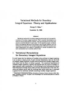
(28) where the Jacobian is assumed constant during the iterative process as long as the number of iterations does not exceed a fixed number. The linear system (28) can be finally solved using a fixed number of block-Gauss–Jacobi (GJ) or blockGauss–Seidel (GS) iterations. More precisely, the coefficient matrix being block-lower-bidiagonal, one iteration of GS will solve (28) exactly, while we assumed that the number of GJ iterations can not exceed six. This choice derives from the experience with the proposed codes and gives the best results in terms of execution time when a relevant number of time steps are considered. The Gauss–Jacobi iterative scheme is based on two levels of iterations: the primary and the secondary iterations. The inner iterative process (i.e., the one relative to the secondary iterations) can be written as Fig. 2. Sequence of parallel operations for the Gauss–Seidel approach.
(29) When convergence is reached for this scheme or the number of GJ iterations exceeds six, the primary iteration can be updated as follows:
The computation is carried out as synthetically shown in Fig. 1. The arrows denote data exchange between processors. A work unit is equal to the central processing unit (CPU) time required to perform a single time step computation. Each processor is devoted to the computation of the variables of a single time step for all the iterations required to achieve the convergence. More time steps may be committed to the same processor if the number of window steps is greater than the number of available processors. To check the convergence, the processors are synchronized after completing the parallel computations relative to the current iteration. The implementation is simple and the expected speed up is of the order of the number of processors. The drawback of the Gauss–Jacobi scheme consists in the need for a “propagation
phase” in which the solution waveform propagates toward the end of the window due to the unidirectionality of the time [12], [13]. This fact increases the number of iterations of the Gauss–Jacobi scheme for long windows. In the tests reported in the next section, we adopted the GS method and hence the solution of (27) is obtained as a limit point in the following linear iteration scheme:
(30) At first glance, the Gauss–Seidel scheme appears to be strictly sequential. It is possible, however, to implement the Gauss–Seidel method in a parallel way as referred to in [14]. The approach was named pipelining-in-time. The computational arrangement is shown in Fig. 2. After computing on processor (i.e., the variables relative at the first time step during the first iteration), the calculation of the second step value can be carried out by processor in
58
IEEE TRANSACTIONS ON CIRCUITS AND SYSTEMS—I: FUNDAMENTAL THEORY AND APPLICATIONS, VOL. 45, NO. 1, JANUARY 1998
parallel with the determination of by . As computation proceeds, the number of time step calculations to be carried out concurrently increases up to a maximum equal to the number of processors. Processors are synchronized after completing a set of concurrent time step evaluations (each time step referring to a different iteration). This synchronization scheme ensures the repeatibility of results. The advantage of the Gauss–Seidel consists, in general, in a reduction of the number of iterations necessary to reach the convergence. This is due to a reduction of the propagation phase [14]. The drawback consists in a speed up lower than the one obtainable theoretically by the use of the Gauss–Jacobi scheme since the solution at different time steps can be updated only sequentially. This drawback can be partially overcome if calculations relative to the previous iteration are performed concurrently in (30). When solving (26), either by the Gauss–Jacobi or by the Gauss–Seidel method, it can be observed that the convergence pattern exhibits a remarkable directionality due to the unidirectionality of the time [12]–[14]. In other words, the convergence of the first time steps of a window always precedes the convergence of the subsequent ones. As in [18], the converged first step of a window can be replaced with the first unassigned time step . The effect is that of having a window moving across the integration time step toward the end of the simulation interval. This approach, named travelling window, permits a significant reduction of the computational effort by eliminating unnecessary iterations on the already converged steps.
considerations shown above on system (28) hold true. For example, if we use the GS method, observing that the Jacobian matrix of coincides with the block-lower-bidiagonal part of , the Jacobian of , the solution of (14) is obtained as limit point of the following linear iteration scheme:
(34) In parallel implementation, (34) does not preserve the strategy of the pipelining-in-time and the travelling window. To avoid this problem, we have suitably modified scheme (34) by means of the following one:
(35) C. Parallel Implementation of ETR4
The iteration process (35) describes a three-step method and belongs to the general class of -step methods. Results on the convergence of such schemes can be found in [34, p. 353]. By numerical tests, we experienced convergence properties of scheme (35) very close to the ones of scheme (34).
In this case, we need to solve the system
(31) We start to analyze the scalar implementation of the code and therefore consider the splitting (22) and consequently the scheme (23) with
(32)
This choice corresponds to consider unknowns in the th equation of (31) and and hence to move all the remaining terms to the right-hand side. Thus, we can rewrite scheme (23) as
(33) of (33), by We get an approximation of the solution means of a single iteration of Newton’s method. The same
VII. PERFORMANCE EVALUATION OF BVM SEQUENTIAL IMPLEMENTATIONS The BVM’s proposed in this paper were tested on a realisticsized network which represents the power system of the midwest of the United States. The test network is characterized by 662 buses and 91 generators. The modeling assumptions reported in [35] were adopted. In particular, a fourth-order model was used for each synchronous machine. Saturation was neglected and system damping was taken into account by introducing a damping factor in the torque equations. Each generating unit was equipped with a fast exciter type IEEE AC4. Finally, loads were represented as algebraic nonlinear functions of the voltage magnitude. In order to produce sufficiently realistic software, state-of-art sparsity techniques were adopted [1]. Different codes were developed and compared in order to assess the computational performance of proposed BVM’s. For brevity, we report here the results relative to the codes which performed the best. The test results are relative to the following methods: 1) RAM3GS (RAM3GJ) which denotes a code based on the BVM with order-three reverse Adams integration
IAVERNARO et al.: BOUNDARY VALUES METHODS FOR TIME-DOMAIN SIMULATION
rule. The last two letters denote the algorithm adopted for solving the algebraic set of equations, i.e., onestep-Newton–Gauss–Seidel (GS) and the six-stepNewton–Gauss–Jacobi (GJ). 2) ETR#GS (ETR#GJ) which denotes a code based on the Extended TRapezoidal rule. The last two letters denote the algorithm adopted for solving the algebraic set of equations, i.e., one-step-Newton–Gauss–Seidel (GS) and the six-step-Newton–Gauss–Jacobi (GJ). The number # in the acronym denotes the order of the method (2, 4). Note that ETR2GS(GJ) denotes a parallel-in-time algorithm which adopts the classical trapezoidal rule. A conventional step-by-step code was developed in order to compare the results. The algorithm is the so-called Very DisHonest Newton (VDHN) method which gives rise to the best performance in terms of execution time for productiongrade codes. This code was implemented following the same algorithmic features of the one described in [34]. In this method, the trapezoidal rule is used to discretize the differential equations of (2.1) which are solved along with the algebraic network equations by Newton type algorithms. The VDHN is basically a modified Newton method characterized by the feature that the Jacobian is held constant over iterations and time steps, as long as convergence is not seriously compromised. Preliminary tests on sequential implementations of BVM’s were conducted on the vector/parallel computer CRAY YMP8/464 used as a conventional computer disabling vectorization and parallelization capabilities. For all tested cases, a three phase fault cleared in 0.06 s was assumed as perturbation cause. The bus fault was located at a bus connected to the generating units which produce the largest amount of power in the test network. Thus, a severe perturbation was considered to evaluate the performance of the proposed algorithms. Tests show that the convergence of the methods is assured for a wide initial-state domain. Some tests with single and double accuracy show that the asymptotic convergence of the algorithms is, in general, consistent with the theoretical expectations. Roundoff errors can cause the slowing down or the loss of convergence when an excessive number of time steps is considered. We compared the algorithms from the viewpoint of the accuracy of the discretization rule. In order to reach this goal, we evaluated the local truncation error (LTE) and the global truncation error (GTE) for simulations with different time steps. The formulas adopted for the evaluation of the LTE are RAM3:
(36)
ETR2:
(37)
ETR4:
(38)
where the derivatives are evaluated, at each time step , numerically with the method of the divided differences [30]. In the following, we always refer to the maximum and minimum value of the LTE, i.e., and , across the trajectory. The GTE was experimentally evaluated comparing the trajectory obtained with the proposed method with a trajectory
59
obtained with the VDHN for a very short step size (0.001 s) and a fixed suitable accuracy for the iterative process. Of course, the GTE refers to selected variables only. In particular, we report the GTE of variables relative at the bus where the short circuit occurs because they are the ones characterized by the highest activity and are the most interesting for judging the stability of the power system. In addition, we evaluated the maximum values of the GTE for the rotor angles (GTE ) and the field voltage (GTE ). The motivation for this choice is that the rotor angle is the variable which one has to look at in order to judge the stability of the power system and the field voltage is the variable associated to the fastest component of the system and the one characterized by a lot of activity in the first instants. Furthermore, about the field voltage GTE we evaluated the GTE in two subintervals: [0, 0.2] s and [0.2, 1] s. This choice is due to the fact that in the period of time in proximity of the fault, exciter windup or nonwindup limiters have a lot of activity introducing discontinuously strong nonlinearities of the saturation type. This effect can not be foreseen by the usual theory on the truncation errors because functions and derivatives are characterized by instantaneous discontinuities whose time of occurrence is not known a priori. Therefore, the GTE evaluated during the second subinterval gives an idea of the truncation error foreseen theoretically, whereas the GTE evaluated on the first subinterval gives an idea of how the BVM methods behave when strong discontinuities are included in the power system model. From Table III, it can be observed that the same order of magnitude of the LTE of the trapezoidal rule (here denoted with ETR2) obtained for s can be obtained using step lengths of 0.04 and 0.06–0.08 s for the RAM3 and ETR4, respectively. This fact has a strong impact on the computational performance as it will be shown in the following. Table III shows how GTE’s are consistent with the LTE’s. The GTE’s relative to the rotor angles are insensitive to the time step length. This is due to the fact that these variables are associated to relatively slow dynamics which could be, in principle, integrated with larger step lengths. The effects of the time step on GTE is more important for the integration of fast variables such as the field voltage as it is illustrated in the column relative to GTE in the interval [0.2, 1] s. In the interval [0, 0.2] s where the activity of the exciter limiters creates discontinuities, the GTE is larger than their respective values in the interval [0.2, 1] s where these effects are damped out. It can be observed that, in some cases, the GTE’s becomes smaller when the step length is enlarged. Although the LTE’s increase as the step length increases, we should recall that the GTE is the cumulative effect of the LTE on all the time steps of the fixed observation interval. Thus, when using a larger step size the number of steps decreases and, as a consequence, the GTE may lower. In Table IV, we compare the proposed algorithms in terms of number of iterations and speed up referred to the VDHN method. The sequential speed up is defined as follows:
run time of the VDHN method run time of the BVM
60
IEEE TRANSACTIONS ON CIRCUITS AND SYSTEMS—I: FUNDAMENTAL THEORY AND APPLICATIONS, VOL. 45, NO. 1, JANUARY 1998
COMPARISON
PERFORMANCES
OF
OF THE
TABLE III TRUNCATION ERRORS
FOR
DIFFERENT BVM’S
TABLE IV PROPOSED ALGORITHMS COMPARED ASSUMING THE STEP SIZE EQUAL TO 0.02 s
In the test results the step size is fixed to 0.02 s for all the algorithms, the integration interval is 1.44 s simulating concurrently 74 time steps. It can be observed that the VDHN method outperforms all the tested algorithms. This is due to the fact that BVM algorithms process concurrently more time steps solving a problem 74 times larger than the one associated to the VDHN method. There are small differences among the wallclock times of the different BVM’s when using the same procedure for solving the nonlinear algebraic problem (namely, the Newton–Gauss–Seidel or the Newton–Gauss–Jacobi). We emphasize that in the ETR4 algorithm the Jacobian has always the same block-bidiagonal structure of the ETR2 because of the application of the splitting illustrated by (24) and (25). Thus, the overhead of ETR4 is only due to a different amount of calculations in the known term of the Newton iteration since the number of steps involved in the integration formulas is different. If a rigorous evaluation of the overall Jacobian were adopted, then a block-quadridiagonal structure would be generated by the ETR4 method increasing markedly the amount of computations per iteration. In Table V, we compare the sequential speed ups and the number of iterations relative to the execution of different codes assuming different time steps and ensuring the same degree of accuracy in terms of LTE as shown in Table III. We adopted the technique described in Section VI about the automatic choice of the step size. Note that some results are not available. This is due to the fact that at least three time steps are needed to
TABLE V PERFORMANCES OF PROPOSED ALGORITHMS COMPARED ASSUMING THE SAME GTE AND DIFFERENT STEP SIZES
implement ETR4 whereas at least two time steps are necessary to apply RAM3. It can be observed that the ETR4GS and RAM3GS have timings comparable with the VDHN for short windows. In particular, ETR4GS is characterized by timings only 20% longer than the VDHN method for a window size of 0.24 s. This result is not negligible because it was obtained solving four time steps simultaneously, i.e., solving, for each window, a problem four times larger than the one solved in conventional step-by-step. VIII. PERFORMANCE EVALUATION OF A PARALLEL/VECTOR IMPLEMENTATION OF BVM’S Results obtained with sequential codes are interesting considering that parallel-in-time algorithms can be implemented
IAVERNARO et al.: BOUNDARY VALUES METHODS FOR TIME-DOMAIN SIMULATION
on parallel machines yielding a speed up due to concurrent processing of time-steps. These methods are characterized by a high efficiency in implementing codes on parallel computers with regard to the performances of parallelized versions relative to step-by-step codes. This is due to the “coarse grain approach” involved in the parallelism-in-time where there is a large amount of calculations associated to each processor compared with the overhead due to communications. The main drawback of the parallel-in-time approach is the software overhead due to the fact these methods solve a larger set of equations than step-by-step codes. The fact that the wallclock time for ETR4GS run on short windows is comparable with the VDHN method is promising for parallel implementations. It should be noted that the Gauss–Seidel versions outperform their respective Jacobi counterparts in a serial environment. This is not necessarily true when applying parallel processing on message passing machine because of the simpler structure of the information flow in Jacobi-type algorithms as proved in [13]–[16] and [18]. However, in Section VII it has been shown that the slow down due to Gauss–Jacobi versions is so high that it would be very difficult to get high performance adopting a limited number of processors. Thus, in the following, we present the implementation of ETR4GS and ETR2GS and compare the results with the VDHN method. A four-processor vector/parallel computer CRAY YMP8/464 was adopted for the implementation of the mentioned algorithms. All test cases were run using single precision arithmetic which is equivalent to the double precision arithmetic of 32-bit computers. Since the number of processors is limited, high performance is achieved by the combined use of parallel and vector processing. It is possible to exploit algorithmic parallelism in the two following ways: • by the concurrent execution of different time steps calculations on the available processors; • by vector processing which is used to speed up the computation of a single time step through the operation pipelining of the vectorizable DO loops. The concurrent execution of different time steps is obtained through the approaches illustrated in Section VI. We remind that the adopted computer is characterized by a shared memory architecture with only four CPU’s. Thus, due to the coarsegrain approach of the parallelism-in-time employed in BVM’s, the shared memory architecture and the small number of CPU’s involved in the concurrent solution of time steps it is foreseeable that memory contention problems can be very limited. Load balancement problems can be considered also minimal since each CPU has to solve a single time step whose computational burden is practically constant. About the application of vector processing the same algorithmic features introduced in [18] were adopted. Vectorizable DO loops were singled out in the computations involved in the block diagonal matrix of the derivatives of synchronous machine equations with respect to state variables, in the computation of network residuals and in the evaluation of the voltage displacement vector by the use of the -matrix method [36].
61
TABLE VI PERFORMANCES OF SELECTED BVM’S IMPLEMENTING PARALLEL/VECTOR COMPUTING
For speed up evaluation, the program VDHN was compiled both enabling the automatic vectorization of the code (version VDHN-V) and disabling vectorization (version VDHN-S). Two speed up values are considered run time of the VDHN-S method on 1 CPU run time of the BVM run time of the VDHN-V method on 1 CPU run time of the BVM The second speed up is introduced to take into account the possibility that the best competitor, i.e., the VDHN method, can also be vectorized on this machine and is a more conservative evaluation of the advantages due to the BVM’s. It is interesting to separately assess the effects that vector and parallel processing have in determining the final speed up value. The speed up is, consequently, expressed as the product of three distinct figures , , and measuring the algorithmic, vectorization, and parallelization speed up, respectively:
where
has been defined in the previous section and BVM run time on 1 CPU BVM to run time enabling vectorization on 1 CPU BVM run time enabling vectorization on 1 CPU BVM run time enabling vectorization on n CPU
The simulation of 1.02 s with a step size of 0.02 s with the VDHN method needs 2.216 and 1.514 s with the VDHN-S and VDHN-V versions, respectively. The step size was chosen on the basis of the accuracy usually required in transient stability codes and the adoption of the conventional trapezoidal rule. In Table VI, the performances of ETR2GS and ETR4GS parallel/vector implementations are evaluated. Results refer to simulations of 1.02 s adopting a different number of CPU’s. Each processor is devoted to the solution of a single time step, thus the window size changes according to the number of processors and the maximum step size compatible with the fixed accuracy. Note that in the case of ETR4GS results relative to 1 or 2 CPU’s are not available since this discretization rule can be applied only in the case the number of time steps to be processed concurrently is least 3.
62
IEEE TRANSACTIONS ON CIRCUITS AND SYSTEMS—I: FUNDAMENTAL THEORY AND APPLICATIONS, VOL. 45, NO. 1, JANUARY 1998
ETR2GS was run with a step size s which was the maximum value compatible with LTE’s usually required for transient stability analysis. ETR4GS was run with a step size of 0.02 s to compare its timings with the ones obtained with ETR2GS on the same basis. A more fair comparison between the two codes, however, consists in analyzing timings on the basis of the same LTE. On the basis of Table III, this implies that ETR4GS can be run with a step size of 0.06 s giving rise to LTE’s comparable with the ones obtained with ETR2GS using a step size of 0.02 s. From test results relative to ETR2GS, it can be noted that as long as the number of time steps processed concurrently increases the sequential speed up decreases due to the increase of the size of the problem but the cumulative effect of and is such that the overall speed up always increases. The code ETR4GS run with a step size of 0.02 s exhibited a lower sequential speed up with regard to ETR2GS since a higher number of calculations was needed to implement a more complex integration rule. This overhead was partially counterbalanced by slightly higher vector and parallel speed ups due, also in this case, to a higher number of calculations associated to ETR4GS. In fact, the increase of computations enlarges the grain of the problem causing an improvement of the performances of vectorization and parallelization. The best results were obtained with ETR4GS run on a grid characterized by a step size of 0.06 s. This is mainly due to a higher sequential speed up . A slight improvement of vector and parallel speed up is due to the fact that more computations are needed to evaluate a single step of ETR4GS than the ones necessary when using ETR2GS. The synergy between vectorization and parallelism-in-time attains a speed up in excess of 25 which is the best result reached up to now for transient stability analysis. Also the speed up evaluated taking into account the vectorization of the VDHN code is significant and equal to 17. Timings obtained with ETR4GS are also interesting for online applications since they show the possibility of running several hundreds of contingencies every 10–15 min, which is what usually required in dynamic security assessment. IX. CONCLUSIONS In this paper, the class of BVM-based algorithms for solving the transient stability problem by exploiting parallelism across time steps is proposed. Some BVM integration formulas result suitable for transient stability analysis because they can solve stiff problems ensuring the same stability features of the trapezoidal rule. Particular care should be put in choosing formulas which avoid hyperstability problems such as the proposed extended trapezoidal rules. BVM’s consent to overcome the Dahlquist barrier guaranteeing A-stability together with order of accuracy higher than two. This is an important result because allows larger time steps to be used reducing execution time with regard to other parallel-in-time algorithms. The existence, the uniqueness and the convergence properties of the numerical solution obtained by Newton/relaxation algorithms have been demonstrated for nonlinear DAE’s.
The best choice among the proposed BVM’s is the extended trapezoidal rule of order four with the implementation of a block-Newton–Gauss–Seidel algorithm. The joint use of a moderate degree of parallelism-in-time and vectorization increases several times the speed up obtainable by traditional techniques of vectorization. The synergism obtainable by the two approaches permit to reach a sufficiently high speed up for online implementations of power system transient stability analysis. ACKNOWLEDGMENT The encouragement and the contribution of G. P. Granelli and M. Montagna in implementing on a Cray machine the proposed BVM’s is gratefully acknowledged by the authors. REFERENCES [1] B. Stott, “Power system dynamic response calculations,” Proc. IEEE, vol. 67, pp. 219–240, Feb. 1979. [2] M. Stubbe, A Bihain, J. Deuse, and J. C. Baader, “STAG: A new unified software program for the study of the dynamic behavior of electrical power systems,” IEEE Trans. Power Syst., vol. 4, pp. 129–138, Feb. 1989. [3] H. Fankhauser, K. Aneros, A. Edris, and S. Torseng, “Advanced simulation techniques for the analysis of power system dynamics,” IEEE Comput. Applicat. Power, vol. 3, pp. 31–36, Oct. 1990. [4] J. Y. Astic, A. Bihain, and M. Jerosolimski, “The mixed AdamsBDF variable step size algorithm to simulate transient and long-term phenomena in power systems,” IEEE Trans. Power Syst., vol. 9, pp. 929–935, May 1994. [5] D. E. Barry, C. Pottle, and K. Wirgau, “A technology assessment study of near term computer capabilities and their impact on power flow and stability simulation program,” EPRI-TPS-77-749, Final Rep., 1978. [6] J. Fong and C. Pottle, “Parallel processing of power system analysis problems via simple parallel microcomputer structures,“ EPRI-EL-566SR, 1977. [7] R. Podmore, M. Liveright, S. Virmani, N. M. Peterson, and J. Britton, “Application of an array processor for power system network computations,” in IEEE Power Industry Computer Applications Conf., Cleveland, OH, May 1979, pp. 325–331. [8] F. M. Brasch, J. E. Van Ness, and S. C. Kang, “Design of multiprocessor structures for simulation of power system dynamics,” EPRI-EL-1756, 1981. [9] C. W. Gear, “The potential of parallelism in ordinary differential equations,” Dept. Comput. Sci., Univ. Illinois, Urbana-Champaign, Rep. R-86-1246. [10] IEEE Committee Rep., D. J. Tylavsky and A. Bose, Co-Chairmen, “Parallel processing in power system computation,” IEEE Trans. Power Syst., vol. 7, no. 2, pp. 629–638, May 1992. [11] M. La Scala, A. Bose, D. J. Tylavsky, and J. S. Chai, “A highly parallel method for transient stability analysis,” IEEE Trans. Power Syst., vol. 5, pp. 1439–1446, Nov. 1990. [12] M. La Scala, A. Bose, and D. J. Tylavsky, “A relaxation type multigrid algorithm for power system stability analysis,” in IEEE Proc. Int. Symp. Circuits and Systems, Portland, OR, May 1989, vol. 3, pp. 1954–1959. [13] M. La Scala, M. Brucoli, F. Torelli, and M. Trovato, “A Gauss–Jacobi–block–Newton method for parallel transient stability analysis,” IEEE Trans. Power Syst., vol. 5, pp. 1168–1177, Nov. 1990. [14] M. La Scala, R. Sbrizzai, and F. Torelli, “A pipelined-in-time algorithm for transient stability analysis,” IEEE Trans. Power Syst., vol. 6, pp. 715–722, May 1991. [15] N. Zhu, J. S. Chai, A. Bose, and D. J. Tylavsky, “Parallel Newton type methods for power system stability analysis using local and shared memory multiprocessors,” IEEE Trans. Power Syst., vol. 6, pp. 1539–1545, Nov. 1991. [16] M. La Scala and A. Bose, “Relaxation/Newton methods for concurrent time step solution of differential-algebraic equations in power system dynamic simulations,” IEEE Trans. Circuits Syst., vol. 40, pp. 317–330, May 1993. [17] M. La Scala, G. Sblendorio, and R. Sbrizzai, “Parallel-in-time implementation of transient stability simulations on a transputer network,” IEEE Trans. Power Syst., vol. 9, pp. 1117–1125, May 1994.
IAVERNARO et al.: BOUNDARY VALUES METHODS FOR TIME-DOMAIN SIMULATION
[18] G. P. Granelli, M. Montagna, M. La Scala, and F. Torelli, “RelaxationNewton methods for transient stability analysis on a vector/parallel computer,” IEEE Trans. Power Syst., vol. 9, pp. 637–643, May 1994. [19] A. O. H. Axelsson and J. G. Verwer, “Boundary value techniques for initial value problems in ordinary differential equations,” Math. Comput., vol. 45, no. 171, pp. 153–171, July 1985. [20] L. Lopez and D. Trigiante, “Boundary value methods and BV-stability in the solution of initial value problems,” Appl. Num. Math., vol. 11, pp. 225–239, 1993. [21] P. Marzulli and D. Trigiante, “Stability and convergence of BVMs for solving ODEs,” J. Difference Equations and Applicat., vol. 1, pp. 45–55, 1995. [22] P. Amodio and F. Mazzia, “Boundary value methods for the solution of differential-algebraic equations,” Numerische Mathematik, vol. 66, pp. 411–421, 1994. [23] , “A boundary value approach to the numerical solution of IVP by multistep methods,” J. Difference Equations and Applications, vol. 1, pp. 353–367, 1995. , “Boundary value methods based on Adams-type methods,” Appl. [24] Numer. Math., vol. 18, pp. 23–35, 1995. [25] C. W. Gear and L. R. Petzold, “ODE methods for the solution of differential/algebraic systems,” SIAM J. Numer. Anal., vol. 21, no. 4, pp. 716–728, Aug. 1984. [26] J. C. P. Miller, “Bessel functions—Part II,” Math. Table, X, British Association for the Advancement of Sciences, Cambridge Univ. Press, 1952. [27] F. W. Olver, “Numerical solution of second order linear difference equations,” J. Res., vol. 71B, pp. 111–129, 1967. [28] A. Carasso, “Long-range numerical solution of mildly nonlinear parabolic equations,” Numer. Math., vol. 16, pp. 304–321, 1971. [29] J. R. Cash, Stable Recursions. New York: Academic, 1976. [30] J. D. Lambert, Computational Methods in Ordinary Differential Equations. New York: Wiley, 1985. [31] L. Brugnano and D. Trigiante, “High order multistep methods for boundary value problems,” Appl. Numer. Math., vol. 18, pp. 79–94, 1995. [32] V. M. Ascher, R. M. M. Mattheij, and R. D. Russel, Numerical Solution of Boundary Value Problems for Ordinary Differential Equations. Englewood Cliffs, NJ: Practice-Hall, 1986. [33] H. B. Keller, “Numerical solution of two point boundary value problems,” Regional Conf. Series in Appl. Math., CBMS 24 SIAM, 1976. [34] J. M. Ortega and W. C. Rheinboldt, Iterative Solution of Nonlinear Equations in Several Variables. New York: Academic, 1970. [35] “Extended transient-midterm stability package: Technical guide for the stability program,” EPRI EL-2000-CCM-Project 1208, Jan. 1987. [36] M. K. Enns, W. F. Tynney, and F. L. Alvarado, “Sparse matrix inverse factors,” IEEE Trans. Power Syst., vol. 7, pp. 466–473, May 1990.
63
Felice Iavernaro received the degree in mathematics from the University of Bari, Italy, in 1991. He has been Assistant Professor at the same university since 1994.
Massimo La Scala (S’88–M’89) received the degree in electrical engineering in 1984 and the Ph.D. degree in 1989 from the University of Bari, Italy. He joined the Italian Power System Board (ENEL) in 1987, was Assistant Professor at the University of Bari from 1990 to 1992, and Associate Professor of Power System Automation in the Department of Electrical Engineering, University of Naples, Italy, from 1992 to 1996. Recently he joined the Department of Electrical Engineering, Politecnico di Bari. Prof. La Scala is member of the IEEE Power Electronics Society and Associazione Elettrotecnica ed Elettronica Italiana (AEI).
Francesca Mazzia received the degree in computer science from the University of Bari, Italy, in 1989. She has been Assistant Professor at the University of Bari since 1990. Ms. Mazzia is a Member of SIAM (Society for Industrial and Applied Mathematics).