Bounded Rationality and Imperfect Learning: Game Theory vs AI¤

Bounded Rationality and Imperfect Learning: Game Theory vs AI¤ Philippe Jehiely June 2003

Abstract This paper reviews three game theoretic solution concepts with boundedly rational players assumed to have imperfect learning abilities: the limited foresight equilibrium (Jehiel 1995), the analogy-based expecation equilibrium (Jehiel 2000) and the valuation equilibrium (Jehiel and Samet 2003). It then reviews the relation of these concepts to some ideas developed in Arti¯cial Intelligence for game playing programs. Key words: Game theory, AI, bounded rationality, learning. Journal of Economic Literature Classi¯cation Numbers: C72, D81.

¤I

would like to thank Daniel Zizzo and an anonymous reviewer for improving the clarity of

the paper. y CERAS, Paris and UCL, London. mailing address: C.E.R.A.S.-E.N.P.C., C.N.R.S. (URA 2036), 48 Bd Jourdan, 75014 Paris, France; e-mail: [email protected].

1

1

Introduction

From a theoretical viewpoint, games like Chess, Checkers or Go have a very simple structure: they are ¯nite horizon games with perfect information. Game theory informs us that these games have a solution that can be obtained inductively from the ¯nal leaves of the game tree working backwards. But, no player however sophisticated can solve such games. More importantly, standard theory and its backward induction technique are of little help to understand how real players behave in such games. Thus, there is a need to develop theories that incorporate bounded rationality into game theoretic setups. There are obviously many facets to bounded rationality (see Rubinstein 1998 for a review of a number of game theoretic approaches other than the ones developed here). The viewpoint adopted in this paper is that players have imperfect learning capabilities. Following previous work (Jehiel 1995, Jehiel 2000 and Jehiel and Samet 2003) this paper considers three classes of learning imperfections, and it illustrates for each class of imperfections the corresponding equilibrium concepts that stand for the limiting outcomes that would emerge after (imperfect) learning has taken place. Speci¯cally, I consider in turn the e®ects of limited foresight - which stipulates that in long horizon contexts players make forecasts only about the near future (Jehiel 1995) - the e®ects of analogy-based expectation formation - which stipulates that players learn only the average reaction function of their opponents over bunches of situations (as opposed to for every single situation) (Jehiel 2000) - and the e®ects of similarity-grouping in reinforcement-like learning situations - which stipulates that players learn the valuations of classes of moves (as opposed to valuations of every single move) (Jehiel and Samet 2003). I illustrate the working of the three approaches in simple examples. Somehow the main motivations in these game-theoretic approaches share some similarity with that branch of Arti¯cial Intelligence interested in game-playing programs (AI is precisely concerned with those problems that cannot be solved 2

explicitly - See, for example, Pearl 1984). In the second part of the paper, I review a number of ideas developed for the game-playing program AI literature, in particular, the notion of board valuation in chess or checkers, the bounded lookahead technique, the deep search pathologies. Then I discuss their relationship with the previously introduced game-theoretic approaches.

2

Three Game-theoretic Approaches

In this section I review three solution concepts with boundedly rational players who are assumed to have imperfect learning abilities.

2.1

Limited Foresight Equilibrium (Jehiel 1995)

In a limited foresight equilibrium, players do not know the reaction of their environment in a distant future. Yet, players are assumed to know the game tree. At each decision node, players solely base their decisions on forecasts about what will happen in the near future, and players' forecasts are assumed to include their own actions. Any equilibrium is parameterized by the number of periods players look ahead. At any point where they must move players choose actions that look best given their forecasts, and equilibrium forecasts are correct. In Jehiel (1995 and 1998) I have considered repeated alternate-move games in which the criterion used by the players coincides with the sum of payo®s received within the horizon of foresight.1 But, the approach can be applied more broadly provided a reasonable criterion based on the limited horizon forecast is available. To understand the idea of the limited foresight equilibrium (Jehiel 1995), it is instructive to consider a one-person decision problem as depicted in Figure 1 (the example is adapted from Jehiel and Lilico 2002). 1 In

Jehiel (2001), I looked at repeated games and considered stochastic criteria (to re°ect

the noisy attitude toward unpredicted components).

3

-1/2 2 -1 0 0

2

-1

1

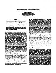
Figure 1: A Simple Decision Problem Each circle represents a point at which an action is to be taken. The branches of the tree represent those actions, and at the ¯rst two decision-points the agent can choose to go Up or Down in the tree. Branches which have no sub-branches represent terminal nodes. The decision-maker receives payo®s after each action corresponding to the numbers shown in the Figure. Suppose that the decisionmaker can see ahead one period.

Then from period one he can see that if he

goes Down to start with he will receive a payo® of 1 and the game will end, while if he chooses to go Up then he will be able to choose between a payo® of 2 if he goes Up at his second decision node and 0 if he goes Down. Under the limited foresight equilibrium concept I have in mind an agent who is aware of his limited foresight. He has perhaps played the game many times before, and is aware that, from this situation, if he were to choose to go Up at the ¯rst decision-point, he would then choose to go Down at the second.2 He is not sure why he would do this, i.e. he does have limited foresight. But he has learned that would be his behavior, and what he has learned is correct. To ¯x ideas, I will assume that when the agent makes no prediction about a decision 2 He

would go down because at the second decision-point 0+max(2; ¡1) > 2+max(¡0:5; ¡1):

4

to be made too far ahead (beyond his horizon foresight), he puts equal weight on all feasible actions. So at the ¯rst decision point the agent believes that he is choosing between going Down and receiving a payo® of 1, or going Up and receiving a payo® of 0 this period and next period while being uncertain as to whether he will go Up or Down in the third period. Thus his valuation of Up is 0+0+

2¡1 2

= 1=2, and given his valuation of Up (which is 1) he goes Down at

the ¯rst decision node. Hence, in the limited foresight equilibrium, strategy is (Down, Down, Up, Up). Note that this is di®erent from the sub-game perfect strategy, which is (Up, Down, Up, Up).

2.2

Analogy-based Expectation Equilibrium (Jehiel 2000)

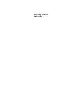
In an analogy-based expectation equilibrium, players do not perfectly distinguish the various possible scenarios when forming their expectations about the behavior of their opponents. Players base their strategies solely on expectations about the average play of their opponents over bunches of situations. Equilibria are parameterized by how players group contingencies to simplify their expectation problem. Each group of contingencies is referred to as an analogy class. In equilibrium, players choose best-responses to their analogy-based expectations and expectations correctly represent the average behavior of the opponents over each analogy class. To illustrate the approach (Jehiel 2000) consider the two-person extensiveform game depicted in Figure 2.

5

A

B

A

R

P1

P2

T1

T2

( -1,0)

P3

(0,4)

T3 (2,1)

(8/3,2)

Figure 2: A Simple Extensive Form Game Players play in alternate order. Player A plays twice, in the ¯rst and third period. Player B plays in the second period. At each time where they must move players may either pass or take - actions in period k are denoted by Pk, Tk, and they are identi¯ed with the corresponding successor in the game tree - (R is the root of the game tree). Payo®s are delivered when a ¯nal leaf of the tree is reached and players' payo®s are as shown in the Figure. In the standard rationality paradigm (i.e., in the unique Subgame Perfect Nash Equilibrium), player A takes in period 3, player B takes in period 2 and player A passes in period 1. This can easily be seen by the use of the backward induction technique. In the analogy approach, suppose that player B does not distinguish periods 1 and 3 when he tries to form an expectation about player A's behavior. That is, player B is assumed to bundle period 1 and period 3 into a single analogy class to predict the behavior of player A. In such a scenario, the following strategies form an equilibrium (in fact, it is the only one): player A passes in period 1, and takes in period 3; player B passes in period 2. A notable di®erence with the Subgame Perfect Nash Equilibrium is that player 6

2 passes in period 2 instead of taking, thus resulting in a ¯nal outcome T3 instead of T2. The main reason why he does so is that player B expects player A to play half of the time pass and half of the time take on average all over the game. Indeed such an expectation correctly represents the average behavior of player A given the strategies: when in period 1, player A passes; when in period 3, player A takes; and the equilibrium frequencies of the game being at periods 1 and 3 are the same (given that player 2 passes with probability 1 in period 2). Finally, observe that given his expectation, player B ¯nds it best to pass at his decision node, since 21 (1 + 4) > 2.3 Observe that the theory does not require the players to know the payo®s of their opponents nor how opponents group contingencies into analogy classes. It only requires that players know the move structure and their own payo®s. The rest of the closing of the equilibrium requirement is (assumed to be) managed through the working of the learning process.4

2.3

Valuation Equilibrium (Jehiel and Samet 2003)

In a valuation equilibrium, players do not form expectations about their opponents' behavior. Instead, they assess the strength of the various available moves according to the valuation (or induced payo®) they receive from choosing the move. But, players do not have separate valuations for every single move. They bundle together several moves they may choose at the various decision nodes and they attach valuations only to bundles. Again equilibria are parameterized by how players bundle moves, and each bundle of moves is referred to as a similarity class. In equilibrium, at each decision node, players choose a move that belongs 3 Player 4 This

B believes that if he passes, the ¯nal outcome will be P3 or T3 with equal probability. comment is very much in the spirit of Kalai and Lehrer (1993) who observe in a

rational learning context that players need not know the payo® structure of their opponent to get convergence to Nash play.

7

to a reachable5 class with highest valuation, and the valuation of each similarity class is assumed to coincide with the average payo® obtained by the player conditional on some move in the class being chosen (Jehiel and Samet 2003). To illustrate the approach consider again the two-person extensive-form game depicted in Figure 2. Suppose that player A assigns the moves P1 and P3 to the same similarity class referred to as P. Suppose further that all other moves T1, T2, T3, P2 belong to singleton similarity classes (they each have separate valuations). In such a scenario, the following strategies form an equilibrium (in fact, it is the only equilibrium): player A passes in period 1; player B passes with probability 1/2 and takes with probability 1/2 in period 2; player A passes with probability 1/3 and takes with probability 2/3 in period 3. Note that we get an equilibrium involving randomization by both players. Thus, the approach leads to a prediction that di®ers from those of the Subgame Perfect Nash Equilibrium or the Analogy-based Expectation Equilibrium.6 To see that the above strategies constitute an equilibrium, note ¯rst that player A's valuations of T1, and, T3 are ¡1 and 2, respectively. Player B's valuations of T2 and P2 are 2 and

2 3

¢1+

1 3

¢ 4 = 2, respectively. To calculate

player A's valuation of P, we need to calculate the relative frequencies of visits of each of the ¯nal leaves T1, T2, T3 and P3 being reached conditional on either P1 or P3 being played by player A. Clearly, T1 is never reached and 21 ; 13 ; 16 are the respective probabilities that the ¯nal leaf T2, T3, P3 is reached (conditional on P1 or P3 being played). Thus, player A's valuation of P is

1 2

¢ 83 + 13 ¢ 2 + 16 ¢ 0 =

2. Given these valuations, player A ¯nds it optimal to pass at period 1 (since vA (P ) = 2 > vA (T 1) = ¡1), and he is indi®erent as to whether to pass or take at 5A

similarity class is said to be reachable if there is an accessible move that belongs to that

class. 6 If players A and B have limited foresight and see one period ahead only, the equilibrium coincides with the Subgame Perfect Nash Equilibrium in this example.

8

period 3 (since vA (P ) = vA (T 3) = 2) (so it is a best-response to mix at period 3 as explained above). Given player A's strategy at period 3, player B is indi®erent as to whether to take or pass at period 2 (since vB (T 2) = vB (P 2) = 2), so his behavior is optimal, and the strategies above constitute an equilibrium. Observe that the theory does not require the players to know the structure of the game nor how opponents group their moves into similarity classes. The closing of the equilibrium requirement is again (assumed to be) managed through the working of the learning process.

3

The AI approach

The aim of this Section is to review some of the AI ideas introduced for gameplaying programs and discuss their relationship to the models of bounded rationality introduced above. It should be mentioned that this review does not include ideas developed in the connectionist AI approach (for such approaches, see Zizzo and Sgroi (2000) and Sgroi (2003)). The starting point of AI is an interest in those problems whose explicit solutions are too hard to derive. AI then moves on to suggest heuristics that are meant to approximate the solution. A ¯rst di®erence between game theory and AI is that the aim of the former is to provide adequate representations of how real subjects behave in strategic interactions7 whereas the aim of AI is to provide satisfactory solutions to complex problems. But, AI soon realized the advantage of incorporating into the heuristics some elements inspired from how human beings seem to operate in complex environments. The idea was that such elements might improve the performance of AI heuristics as compared with the earlier more mechanical heuristics (or algorithms) considered to be too rigid. So in this sense AI has moved closer to game theory for pragmatic reasons. On the other side, 7 Some

game theorists may regard the purpose of game theory in a more normative way (as

providing clues about how rational players should behave).

9

the interest of game theory in bounded rationality (in particular the approaches described above) precisely lies in the acknowledgment that some environments are too complex for the traditional game theory approaches to be descriptively accurate. In this sense, the game theory agenda has moved closer to that of AI. It should also be mentioned that the game-playing programs considered in AI mostly (if not always) concern zero-sum games with two players who move in alternate order (like chess or checkers). By contrast, the game theoretic approaches described above make no such restrictions. The focus on zero-sum games will explain some of the modeling choices made in the AI literature.

3.1

Valuations

An insight that can be derived from Zermelo's algorithm is that, in (generic) ¯nite horizon extensive form games with complete information, every node has an unique (equilibrium) value for every player that can be determined backwards from the ¯nal leaves of the game tree. In short, Zermelo's algorithm can be described as follows. Clearly, at a terminal node, the values are determined by the payo®s of the game. For an immediate predecessor of a terminal node, it is anticipated that the player who must play will choose a move leading to a terminal node with maximum value for him. This in turn determines values for this node. And so on backwards for every node of the game tree. But, in complex games such as checkers, go or chess, Zermelo's algorithm is not operational because there are far too many nodes, and it is thus of little help to compute the equilibrium value of every board position (except very close to the end). An alternative for example in checkers is to consider a list of criteria such as (1) the "pieces ahead" criterion - this is in checkers the number of pieces the player has in excess of his opponent or (2) the "moments about the center" criterion - this is a measure of the number of pieces of each player about the center (see for example, Holland (1998) chapter 4). In chess, the pieces ahead

10

criterion can be re¯ned to adjust for the relative strengths of the various pieces. Then one can aggregate the above criteria - for example using a weighted sum of the individual criteria - which in turn de¯nes a valuation. The valuations so de¯ned can be used to assess the strength of the various positions. A simple heuristic for playing a game is then to choose a move leading to a position with highest valuation. (The ¯rst game playing program with this feature and many others - some of which to be discussed later - has been introduced for checkers by Samuel 1959.) The above heuristic leaves aside two important elements: (1) How are the basic criteria to be derived/guessed in the ¯rst place? (2) How are the weights between the various basic criteria determined? Regarding (1) no clear view seems to prevail. I guess that a plausible view might be that the intuition of real (preferably master) players is used to determine which criteria seem more adapted. Regarding (2) the basic (often implicit) AI idea here is that as many games get to be played and recorded one gets a better idea of the chance of winning as a function of the various criteria. Making statistics over these allows in turn the researchers/programmers to adjust the weights between the various criteria in a consistent way (that is, in a way that re°ects the long run frequencies of win as a function of the pro¯le of realizations of the various criteria). We now turn to the connection of such heuristics to the game theoretic approaches developed in Section 2. Observe ¯rst that the valuation approach has some connection with the idea of reinforcement learning ¯rst introduced in psychology by Bush-Mosteller (1955) and recently popularized in game theory by Erev and Roth (1999) which stipulates that strategies are solely assessed according to how well they perform (as opposed to whether they are best-responses to expected strategies of the opponents). But, the valuation approach as described above somehow views the moves and not the strategies as being the subject of reinforcement (the strategy in games like checkers are too complex to be directly the subject of reinforcement). 11

Sutton and Barto (1998) describe (for tic tac toe) reinforcement learning models of this sort in which the valuations of moves are the subject of reinforcement, and the valuations of the various moves are treated separately. The convergence properties of these learning dynamics have been studied only recently in gametheoretic contexts by Jehiel and Samet (2000). However, the AI approach based on (linear) aggregations of the basic criteria does not treat the valuations of every board position separately. By making the valuation a sole function of a few limited number of criteria the approach implicitly assumes that many board positions are pooled together: all those positions for which all individual criteria coincide must have the same valuation. In this sense, the approach has close connections with the valuation equilibrium approach (Jehiel and Samet 2003) explained above.8 A further connection is about how the valuations attached to the various similarity classes are assumed to be consistent in Jehiel and Samet (2003) and how the weights attached to the various basic criteria are assumed to respect the observed long run frequencies of Win.9 A small di®erence though is that the AI approach in general restricts attention to valuation functions that are linear interpolations between the various basic criteria, an extra constraint that does not appear in the valuation equilibrium approach. To some extent, the analogy-based expectation equilibrium (ABE) approach can be viewed as the belief-based counterpart of the valuation equilibrium (VE) approach (note that ABE was introduced before VE). In the analogy-based expectation equilibrium approach, players form expectations about the reaction function of other players; they group together many situations (into analogy classes) 8 At

¯rst glance, it might be objected that the AI approach considers the valuation of the

board positions rather than the valuation of moves. But identifying the valuation of the move with the valuation of the board position it leads to reveals that there is an equivalence between the two. 9 The consistency feature is, of course, shared by all three game theoretic approaches in the previous Section.

12

and they try only to learn the average reaction function in each pool. The pooling of situations make in turn learning more manageable because in particular many more data are available. The pooling is clearly a feature common to the AI approach and the ABE and VE approaches. Some researchers have tried to assess the relative adequacy of belief-based learning versus reinforcement learning on experimental grounds (see Camerer and Ho 1999 for some experimental account in simple normal form games).10 But, in my opinion the relative adequacy of the two approaches very much depends on the kind of feedback that subjects receive (and/or focus on) at the learning stage. If the main feedback is about players' own payo®s then presumably reinforcement learning models are more adapted. If the main feedback is about the behavior/reaction of the opponents (whereas players' own payo®s are not immediately available, say) then belief-based learning seem more appropriate. When the two types of feedback are available then a mixture of the two may be a better modeling representation. To summarize, depending on the feedback scenario, the corresponding boundedly rational equilibrium concept (SVE or ABE or a mixture of the two - to be de¯ned) may be more appropriate.

3.2

Bounded look-ahead

An extension of the valuation approach suggested above is not to use the valuation immediately, but use it after the play has continued through several rounds of moves and counter-moves. The idea is to expand a portion of the game tree up to a given depth and then use the valuation in order to assess the merit of the board positions on the search frontier. Then the game is solved by backward induction as if the true values of the frontier nodes coincided with the valuations. In turn 10 Most

of the game theoretic literature on reinforcement learning considers the reinforcement

of actions. There are only few attempts to consider the reinforcement of rules instead (an exception is Stahl (2003)).

13

the backwards induction argument leads to a choice of action at the current (root) node. Note that in the backward construction it is assumed that when it is the opponent's turn to move the opponent chooses the action which minimizes the ensuing valuation of the player. That technique is referred to in AI as the bounded look-ahead technique (see Pearl (1984) subsection 8.1.2.) and it was proposed as early as 1950 by Shannon. At ¯rst glance there is a close connection between the idea of bounded lookahead such as considered in the AI literature and the idea of limited foresight in games such as de¯ned above. Yet, there are important di®erences as we now explain. First, strictly speaking the lookahead method applies only to zero-sum games, since assuming that the opponent minimizes the player's valuation can only make sense in such settings. As a matter of fact even in zero-sum games, assuming the opponent minimizes the valuation is debatable. Indeed, there is no reason (1) why player j would use as her valuation function the opposite of the valuation function of player i - valuations are player-speci¯c approximations of the true objective functions and these approximations have no reason to be the same across players- and (2) why player j would rely exactly on the same expansion depth of the game tree as player i -players may di®er in their ability to expand the game tree. I think the AI literature is well aware that the lookahead method relies on a rather crude modeling of the opponent. An interesting defense proposed in favor of the method heavily relies on the zero-sum character of the considered games. Suppose the valuations used by player i are good approximations of the true Win/Loss assessments of the various board positions. Then the look-ahead procedure leads to a strategy for player i that is the correct one assuming that both players i and j can solve the game perfectly. Because we have a zero-sum game, by following this strategy player i can secure the (rational) equilibrium value outcome even if player j were to follow another suboptimal strategy (this 14

is a corollary of the minmax theorem). Of course, in some cases if player j plays suboptimally and had player i anticipated the poor behavior of player j he could have achieved a better outcome. But, if one looks for solutions that perform well against good players (presumably the main focus of AI), the argument even though partial has some appeal. The lookahead method is then viewed as a cautious one, since interpreting the valuation function of player i as the best (available) proxy for the true value function it assumes that player j can use the same (equally good) proxy. It should be noted that to the best of my knowledge the AI literature does not discuss the possibility (and implication) that the opponent may use a di®erent expansion depth of the game tree. The idea of cautiousness that underlies the above discussion does not carry over to games which do not possess a zero-sum structure. Adapting the lookahead method to more general (non-zero sum) games would require that each player i endows other players j with valuation functions of their own. While in some cases players may have some estimates about the valuations of their opponents (in particular when individuals play both the roles of players i and j at di®erent points in time), in other applications it may be hard for a player to have access to the valuation functions of their opponents (the payo®s derived by the other players is not even observable in many economic applications). When players do not have access to the valuations of their opponents, a modi¯ed look-ahead technique might be considered in which players now base their decisions on their estimates about how their opponents might react over a given depth expansion of the game tree. The idea is as follows. Player i holds some theory about which (distribution of ) moves his opponents will choose at each possible con¯guration over a ¯nite depth expansion of the game tree. Together with his valuations to assess the strengths of the frontier nodes, player i can solve backwards for the best move to make at each position within the truncated game tree assuming player j will react according to the theory and player i will each 15

time select the move leading to the highest (expected) valuation at the frontier. An equilibrium concept along these lines would require that player j's reaction function assumed by player i correctly represents the true behavior of player j within the given depth expansion. The induced solution concept bears some similarity with the one considered in Jehiel (1995) with a signi¯cant di®erence to be now discussed. In the limited foresight equilibrium approach introduced in Section 2 the predictions made by each player i includes player i's own actions to be made within the horizon of foresight and not only the actions to be made by other players j within that same period of interaction (as a result the forecasting rules used by the players are less complex objects than say theories about opponents' reaction functions within the horizon of foresight). Including player i's own moves to be made in future stages within player i's horizon of foresight avoids an issue referred to as time inconsistency (Strotz 1956). Because time inconsistencies are hard to justify from a learning perspective, it seems to me that the limited foresight equilibrium approach as de¯ned in Jehiel (1995) is a more sensible way to model equilibrium behavior with limited foresight players (see also Rubinstein 1998 for a discussion). To illustrate the time inconsistency issue, consider the limited foresight oneagent problem of Figure 1. Suppose the agent can see one period ahead and that the agent uses the bounded look-ahead technique just described (i.e., his prediction does not include his own actions to be taken in the next period). The agent would now choose Up at the ¯rst decision node with the plan to play Up in the next node. But, when the second decision node arrives, the agent would play Down. Note that this di®ers from the limited foresight equilibrium described in subsection 2.2 in which the agent plays Down in the ¯rst node because he expects to play Down next if he plays Up in the ¯rst node. The main problem with the look-ahead technique here is that the agent initially chooses to play Up based on the plan that he will play Up next. But, he does not play Up next. When the 16

game is played again and again, the agent is likely to observe that he does not play Up at the second node, and it is then unlikely that the agent will continue to hold the belief that he can stick to the plan of playing Up at the second node. When the agent realizes he cannot stick to his original plan at the second node, the pattern of behavior as resulting from this look-ahead equilibrium is unlikely to remain stable. The limited foresight solution concept does not have this drawback because by construction players behave as predicted within their horizon of foresight.

3.3

Deep-search pathology

Some AI authors (Nau (1980) and Beal (1980)) discovered that in some models of games applying the lookahead technique to deeper expansions of the game tree could degrade the quality of a decision, a phenomenon that Nau termed pathological (see Pearl (1984) chapter 10). In a number of game theoretic contexts, there are examples in which an apparent advantage turns out to be detrimental to the player. Within the game theoretic concepts developed above, Jehiel (1995) provides an example in which a player is worse o® when he has a longer horizon of foresight, Jehiel (2000) provides an example in which a player is worse o® with a ¯ner analogy partition (while the analogy partitions of the other players is assumed to remain the same); Jehiel and Samet (2003) provide an example in which a player is worse o® with a ¯ner similarity partitioning of his moves. At ¯rst glance, the AI deep-search pathology seems related to the ¯nding that a shorter horizon of foresight may in some cases help the player. But, the logic of the two results is completely di®erent as we now explain. An heuristic argument advanced in support of the AI look-ahead technique is the notion of visibility: a position closer to the end (by de¯nition a deeper position in the games of chess or checkers satisfy such a property) is easier to

17

evaluate. This argument is obviously valid when one gets so close to the end game that it is possible to compute the optimal solution. However, in the middle of the game the argument is less transparent. Furthermore, even if the valuation is more accurate going deeper in the game tree, the lookahead technique generates extra errors in the backward construction (because in particular - at least in its most primitive versions - it does not take into account that the valuations at the frontier nodes are themselves subject to errors). The pathologies discovered by Nau typically arise when the valuations at the frontier nodes are not su±ciently more accurate than the immediate static valuations. For the sake of illustration, suppose there is absolutely no improvement of the accuracy of the valuations going deeper. Then the lookahead technique as described above is unlikely to be bene¯cial. Some authors have suggested to modify the lookahead technique by taking into account that the estimates at the frontier nodes are probabilistic (see the product-propagation rules described by Pearl (1984) subsection 10.2.4), which is obviously a way to reduce the pathologies discussed above, at the cost of increased complexity.11 To summarize, the AI deep search pathology is the observation that the lookahead technique generates by itself extra errors, and thus it may sometimes (when going further does not improve signi¯cantly the accuracy of the valuations) deteriorate the quality of the decision as compared with the decision that would have been made without this technique. The logic as to why a player may sometimes (in equilibrium) bene¯t from having a shorter length of foresight is rather di®erent. At ¯rst glance, a longer horizon of foresight is good for a player because he can base his choice of action on a better forecast of the future (and in equilibrium limited forecasts are assumed to be correct). Thus the criterion used by a player with a longer horizon of foresight is closer to his true objective function, and one might have thought that the 11 Other

features like the e®ect of dependencies and the avoidance of traps are discussed as

possible reasons for why the deep search pathology phenomenon may not arise in games like chess or checkers.

18

player should have bene¯tted from it. However, the player, say player i, does not face a ¯xed environment. He plays with (or against) another player, say player j. And this player j will adjust his behavior to a change of behavior of player i (even in the case when player j's horizon of foresight remains the same). For the sake of illustration, consider the following example taken from Jehiel (1995) (see subsection 2.5 of Jehiel 1995 for details): Example: Two players i = 1; 2 play in alternate order. Player 1 chooses each time an action U or D; player 2 chooses between L and R. The stage game payo®s accrue in every period t ¸ 2 are assumed to depend (solely) on the pro¯le of actions chosen at period t ¡ 1 and at period t. There are four possible action pro¯les and the corresponding stage game payo®s for players 1 and 2 are: UL

UR

DL

DR

(1; 1) (2; 2) (3; 5) (1; 6) We assume that players do not discount future payo®s12 , and player 2 can see one period ahead (in the terminology of Jehiel 1995 his length of foresight is 2). We wish to compare the equilibrium payo® obtained by player 1 according to whether player 1 makes no prediction about the future or whether he predicts no less than one period ahead (this is equivalent to perfect foresight here). In the whole exercise, we assume that players' criterion (given their horizon foresight) coincides with the sum of stage game payo®s obtained within the horizon of foresight. When player 1 is myopic, the only equilibrium path is DLDLDL:::, which leads to an average payo® of 3 for player 1. When player 1 has perfect foresight, the only possible equilibrium pattern is DLDRDLDR:::, which leads to an average payo® of

3+1 2

= 2 < 3 for player 1.

So a longer horizon of foresight of player 1 turns out to be detrimental to player 1's equilibrium payo®. The main reason for this result is as follows. When player 1 is myopic, if player 2 chooses R he predicts (rightly) that player 1 will 12 We

could alternatively assume that discounting is very small.

19

choose U next (because 2 > 1). When player 1 is far-sighted on the other hand, player 1 does not choose U after R: this is because player 1 (rightly) expects L to be played next irrespective of his current choice of action and u1 (UR) + u1 (UL) < u 1(DR) + u1 (DL) (2 + 1 < 3 + 1). In turn, player 2 takes advantage of this and plays L and R in alternation while player 1 keeps playing D whenever he has to move. (The complete argument requires checking why player 2 indeed plays L after playing R no matter what player 1 does in between. The dynamic programming technique developed in Jehiel (1995) and (2001) allows us to derive this conclusion.)

Remark: In the above example, player 1 plays D always on the equilibrium path whether he is myopic or he has perfect foresight. Yet, if player 2 were to alternate between L and R when player 1 is myopic, player 1 would no longer play D always. It is the change of player 1's behavior o® the (1; 2)-equilibrium path and player 2's reaction to it that explains the result of the above example.

The general analysis of the circumstances under which a shorter length of foresight may be bene¯cial to a player remains to be done. In the special case of zero-sum two-player games (such as the ones most considered in AI), it is readily veri¯ed that a player with perfect foresight cannot do worse than a player with a shorter horizon of foresight, at least if the opponent has perfect foresight. The point is that, in zero-sum two-player games, a perfectly rational player can always secure his equilibrium value against any behavior of the opponent. Thus, if u1 , u2 are players 1 and 2' equilibrium values of the game (when players are assumed to be rational), player j when rational (i.e. with perfect foresight) gets at least uj in any equilibrium. Since ui = ¡uj is what player i gets when he has perfect foresight, he cannot get strictly more when he has a limited horizon of foresight. The above insight gives some rationale as to why in zero-sum games a greater length of foresight may be desirable. However, the rationale is rather weak be20

cause (1) it only considers a switch from limited foresight to perfect foresight (as opposed to a smoother increase of the horizon of foresight) and (2) it assumes that the opponent (player j) has perfect foresight (the argument does not work through if player j has limited foresight). More work is needed to assess when a longer horizon of foresight is desirable, even in two-player zero-sum games.

4

Conclusion

The main achievements of game theory over the past ¯fty years have been to provide the tools for describing the interactions of fully rational players. But, there are obviously many situations, admittedly complex ones, in which full rationality seems out of reach.13 At the same time, AI has developed a long and pragmatic tradition for coping with complex problems. This paper is an attempt to show that the two ¯elds can bene¯t from one another. It is no longer very original to claim that it is now time for game theory to incorporate seriously ideas of bounded rationality. The speci¯c viewpoint of this paper is that it may be fruitful to consider some of the ideas that were ¯rst considered by AI in the context of game playing programs, and incorporate them into game theory.

References [1] Beal, D. [1980], "An analysis of minimax," in Advances in Computer Chess 2, ed. M.R.B. Clarke, pp 103-9. Edinburgh: University Press. [2] Bush, R. and R. Mosteller [1955], "Stochastic Models of Learning," New York: Wiley. 13 Someone

like Simon (see Simon 1955 and the last chapter of Rubinstein 1998) seems rather

skeptical about game theory precisely because of this discrepancy.

21

[3] Camerer, C. and T. Ho [1999]: "Experience-weighted attraction learning in normal-form games" Econometrica 67, 827-74. [4] Erev, I. and A. Roth [1999], "Predicting How People Play Games: Reinforcement Learning in Experimental Games with Unique, Mixed Strategy Equilibrium," American Economic Review. [5] Fudenberg, D. and D. Levine [1998], "The Theory of Learning in Games," The MIT Press. [6] Holland [1998], "Emergence," Addison-Wesley Publishing Company.. [7] Jehiel, P. [1995], \Limited horizon forecast in repeated alternate games," Journal of Economic Theory 67, 497-519. [8] Jehiel, P. [1998], \Learning to play limited forecast equilibria," Games and Economic Behavior 22, 274-298. [9] Jehiel, P. [2000], "Analogy-based expectation equilibrium," mimeo CERAS and UCL. [10] Jehiel, P. [2001], "Limited foresight may force cooperation," Review of Economic Studies 68, 369-391. [11] Jehiel, P. and A. Lilico [2002], "Smoking today and stopping tomorrow: A limited foresight perspective," mimeo CERAS and UCL. [12] Jehiel, P. and D. Samet [2000], "Learning to play games in extensive form by valuation," mimeo CERAS and UCL. [13] Jehiel, P. and D. Samet [2003], "Valuation equilibria," mimeo CERAS and UCL. [14] Nau, D.S. [1980], "Pathology on game trees: A summary of results," Proc. 1st Nat. Conf. on Arti¯cial Intelligence pp. 102-4. 22

[15] Kalai, E. and E. Lehrer [1993], "Rational Learning Leads to Nash Equilibrium," Econometrica 61, 1019-45. [16] Pearl, J. [1984], "Heuristics," Addison-Wesley Publishing Compagny. [17] Rubinstein, A. [1998], "Modeling bounded rationality," The MIT Press. [18] Samuel, A. L. [1959], "Some studies in machine learning using the game of checkers," IBM Journal of Research and Development 3, 211-29. [19] Simon, H. A. [1955], "A Behavioral Model of Rational Choice," Quarterly Journal of Economics 69, 99-118. [20] Shannon, C. E. [1950], "Programming a computer for playing chess," Philosophical Magazine 41, 256-75. [21] Sgroi, D. [2003], "Using Neural Networks to Model Bounded Rational Behavior in Economics," Greek Economic Review, this volume. [22] Stahl, D. O. [2003], "Action-Reinforcement Learning vs Rule Learning," Greek Economic Review, this volume. [23] Strotz, R. H. [1956], "Myopia and inconsistency in dynamic utility maximization," Review of Economic Studies 23, 165-180. [24] Sutton, R.S. and A.G. Barto [1998], "Reinforcement Learning: An Introduction," The MIT Press. [25] Zizzo, D. J. and D. Sgroi [2000], "Emergent Bounded Rational Behavior by Neural Networks in Normal Form Games," Mimeo Oxford University.

23