Consider a two-station tandem system with capacity constraints for at most Ni ...... product-form is violated since when the second station is saturated (n2 = N2), ...
Annals of Operations Research 79(1998)295– 319
295
Bounds and error bounds for queueing networks Nico M. van Dijk Department of Econometrics, University of Amsterdam, Roetersstraat 11, 1018 WB Amsterdam, The Netherlands
Queueing networks are an important means to model and evaluate a variety of practical systems. Unfortunately, analytic results are often not available. Numerical computation may then have to be employed. Or, system modifications might be suggested to obtain simple bounds or computationally easy approximations. Formal analytic support for the accuaracy or nature of such modifications or approximations then becomes of interest. To this end, the Markov reward approach is surveyed and illustrated as a technique to conclude a priori error bounds as well as to formally prove bounds when comparing two related systems. More precisely, the technique can be applied to • perturbations, • finite truncations, • infinite approximations, • system modifications, or system simplifications (bounds). A general comparison and error bound theorem are provided. The conditions and technical steps are illustrated in detail for a non-product form queueing network subject to breakdowns. This illustration highlights the technical difference with and extension of the stochastic comparison approach. In addition, some practical applications are given which illustrate the various types of applications.
1.
Motivation
1.1 Introduction This paper aims to survey and illustrate the Markov reward approach as a technique to formally establish simple bounds and to secure analytic error bounds for simplifying system modifications. The presentation will be tutorial, tailored more to the practical motivation and applications, the difference with stochastic comparison and an illustration of how to verify the technical conditions. The two general theorems that will be provided will therefore be presented in a compact yet self-contained form, with the more technical insights referred to references. First, let us provide some motivational background. © J.C. Baltzer AG, Science Publishers
296
N.M. van Dijk y Bounds and error bounds
1.1.1. Motivational questions Markov chains are known to be powerful modelling tools for a variety of practical situations. Applications are found in telecommunication (queueing networks, broadcasting, satellite communication), computer performance evaluation (computer networks, parallel programming, store and forward buffering), manufacturing (assembly lines, material handling systems), reliability (breakdown analysis), and inventory theory, as well as combinations of these such as performability analysis of computer systems with breakdowns, error detections or fault tolerance. Modelling of realistic situations, however, may itself already introduce inaccuracies by simplifying assumptions and by using estimated values. A perturbation analysis of the errors introduced by these inaccuracies would thus be in place. Traditionally, steady-state behaviour is of prime interest, such as to evaluate a throughput, a blocking probability, a system efficiency, a mean workload, a response time or a system availability. Unfortunately, closed-form expressions for such measures are available only in a limited number of situations (such as a Jackson network without blocking, a finite reversible material handling system, or a simple central processor unit computer system). Numerical or approximate computations may thus have to be performed. These, in turn, easily become astronomic so that a truncation has to be performed. A priori error bounds for the accuracy or order of accuracy of this truncation then become of computational interest. Conversely, on some occasions, infinite systems might lead to simple expressions, for example for the throughput as just the offered workload per unit of time, while for the finite systems such expressions are hard to obtain. An error bound on the accuaracy of an infinite approximation would thus be useful. Explicit steady-state expressions, most notably product-form expressions, for queueing networks are usually obtained only under strong assumptions that are often not satisfied in practice. More precisely, these closed-form expressions are typically violated by practical phenomena such as: • • • •
blocking or dynamic routing, breakdown features, capacity constraints, prioritizations.
On such occasions, it then becomes most appealing to make simplifying assumptions for or modifications of the original system of interest so as to enforce or enable the use of these product-form or related type expressions which lead to simple bounds or reasonable first-order approximations. Two natural questions to justify such an approach thus arise: (i)
When comparing an original with a modified system, most notably to simplify the computations or to justify a simple analytic expression, can we compare the performance of the two systems?
N.M. van Dijk y Bounds and error bounds
297
(ii) And in the same situation or when ignoring some complicating aspects, can we also provide secure (analytic a priori) error bounds on the inaccuracy introduced by the simplification? 1.1.2. Objective This paper aims to illustrate how these two general questions can be addressed more or less in a unified manner by exploiting discrete-time Markov chain properties combined with one-step Markov reward or dynamic programming arguments. 1.1.3. Results • A separate comparison and error theorem will be provided. The essence of these directly related theorems is to analyze steady-state measures by cumulative, Markov reward structures and to apply inductive Markov reward arguments to estimate so-called bias terms. • The technical steps to verify the conditions of these theorems, as well as the possible bounding and error bound results they can lead to, will be illustrated by a practical example. • The two theorems, though in form and technical verification directly connected, are given separately, in order to directly contrast with the more standard stochastic comparison approach. Special attention will be paid to highlight the differences, such as by a listing of advantages and disadvantages. • Three additional applications of practical interest will be provided to further illustrate the potential of the results for practical situations. 1.1.4. Related literature (1) Markov reward approach. The results are directly related to Van Dijk [42] as an extension of an idea developed in Van Dijk and Puterman [44]. The Markov reward technique as employed herein has already succesfully been applied to a number of queueing network situations also without a product form (cf. [40, 41, 43, 46]). The purpose of this paper is to survey and highlight the essential steps as well as the potential of this technique for different purposes, along with insights and contrasting with the standard stochastic comparison approach. In addition, the error bound theorem is given in an extended, more practically useful form by conditioning on an initial steady distribution. (2) Stochastic comparison. The topic of stochastic monotonicity has received considerable attention over the last decade, motivated by the pioneering work of Stoyan [33]. Some notable references here are: Keilson and Kester [19], Massey [18] and Whitt [47, 48]. The results of these references are also directly related to sample path results in combination with
298
N.M. van Dijk y Bounds and error bounds
weak coupling arguments. Typical applications of these results are comparison results for stochastic service or queueing networks as has been extensively studied over the last decade (Adan and Van der Wal [1, 2], Shanthikumar and Yao [28, 29], Tsoucas and Walrand [36], Van Dijk et al. [45]). These stochastic comparison or sample path approaches, however, do not generally lead to error bound results. For comparison purposes, the differences (advantages and disadvantages) with respect to the Markov reward approach will be discussed in more detail in section 2.2. (3) Other error bound results. Numerous approximation results for queueing networks, particularly for assembly-line structures, have been reported over the last decade (see, for example, [3, 6, 10, 11, 13, 23] or Perros and Altiok [21] and references therein). Generally, however, these results do not include analytic or a priori error bounds. In more abstract settings of Markov chain approximations, such error bounds have been reported for specific approximation schemes, such as numerical successive approximation methods and aggregationydisaggregation procedures (cf. [4, 5, 7 – 9, 14, 31, 32, 35]). In fact, also exact analytic expansions for perturbations of a Markov process have been provided (cf. Schweitzer [24], Meyer [20]). In essence, however, these still require an exact computation of the fundamental matrix or relatedly, in the present setting that is, of so-called bias-terms which will be practically infeasible. In this paper, in contrast, just rough bounds for such bias-terms will do. 1.2. Motivational examples In this subsection, we aim to illustrate the motivational questions addressed above by means of concrete queueing network examples which are of practical and computational interest in themselves. We distinguish two cases. (i) A comparison question to guarantee a simple bound (one example). (ii) Error bound questions to establisch accuracy (three examples). 1.2.1. Comparison results and simple bounds A system can be compared under different situations, for example: (1) To investigate the effect of changing certain system parameters such as a storage or service capacity (cf. [1, 2, 28, 34, 45]). (2) To determine a better protocol such as for dynamic job or server allocation (cf. [28]). (3) To conclude that a specific protocol modification leads to a performance bound (cf. [37, 40 – 43]). Let us give an example (see figure 1).
N.M. van Dijk y Bounds and error bounds
299
Figure 1.
Consider a two-station tandem system with capacity constraints for at most Ni jobs at station 1 and N2 jobs at station 2. When station 1 is saturated, arrivals are rejected and lost. When station 2 is saturated, the servicing at station 1 is stopped. This system can be regarded as representative for a variety of applications in manufacturing (assembly lines) and computer performance evaluation (multi-stage processing). Due to the finite constraints, however, it has no product-form expression and a large number of approximation techniques have therefore been developed. These, however, still require restrictive service specifications (such as exponential), are computationally expensive, and last but not least, do not provide any guarantee or error bound. Alternatively, if one is interested in a rough order of magnitude for some global measure such as a throughput or loss fraction, a simple modification might lead to practical results, as will be briefly argued below. The system has no product form as flow balances per station are violated when a saturation occurs (cf. [38]). For example, when station 2 is saturated, at station 1 the outflow becomes 0 while the inflow still remains positive. These flow imbalances are repaired and consequently a product form guaranteed if: • also system arrivals are stopped if station 2 is saturated, • system departures are stopped if station 1 is saturated. Intuitively, this will lead to an overestimation of the loss fraction and thus, by use of the product form, a computationally simple upper bound. Numerical results have illustrated the practical usefulness of these quick bounds (cf. [39, 46]). It is therefore of practical interest to be sure that this modification indeed provides upper bounds, that is to say, to prove the bounds also formally. Established comparison, or relatedly monotonicity, proof techniques such as the one-step comparison technique as employed in [18, 19, 47, 48] and the related sample path technique as in [1, 2, 28, 29, 45], however, do not generally apply. (In fact, for the above intuitive bounds they will fail, as illustrated in [46].) The Markov reward proof technique that will be outlined in this paper has already proven to be a fruitful addition to this end [37, 38, 41, 43] (as will also be shown in section 3). 1.2.2. Error bounds Three examples will be given in which an error bound is of practical computational interest. A first one, when ignoring breakdowns. A second, addressing finite
300
N.M. van Dijk y Bounds and error bounds
truncations or infinite approximations. And a third, in which system protocols are changed. Example 1.2.1: A Jackson network with breakdowns (figure 2). Consider a Jackson network with Poisson arrivals with parameter λ , routing probability pij from station i to station j, p0 j for an arriving job to enter station j and pi0 = [1 – ∑j pij] for a job to leave the system when leaving station i. The service rate at station i is µ i (ni) when ni jobs are present. Furthermore, the system has a finite constraint for no more than M jobs in total. When M jobs are present, an arriving job is rejected and lost.
Figure 2.
In addition, the departure channel of the system is subject to breakdowns, say at an exponential rate β with an exponential repair time at rate σ. When the departure channel is down, a job attempting to leave the system has to remain at the station it came from. Let τ be the fraction of time that the system is down. If τ = 0, in other words, if breakdowns do not occur, it is standard that the system has a simple product-form expression for the steady-state population vector, from which various performance measures L are easily derived. As soon as τ > 0, however, such an expression can no longer be provided and as of today, no analytic expression for the steady-state distribution has been reported. Realistically though, τ should typically be thought of as being quite small, say in the order of 2%, if not far less. It thus seems intuitively appealing to simply ignore breakdowns and to use the results for the product-form model as an approximation. But how good can we guarantee such an approximation to be. In particular, for a performance measure L of interest and with explicit constant C, can we provide an a priori error bound of the form |Lτ > 0 – Lτ =0| ≤ τ C. Example 1.2.2: Finite or infinite approximation (figure 3). (i) A finite truncation ( figure 3(a)). Again, consider an arbitrary queueing network that has no product form such as in figure 3(a), where jobs are rerouted to an overflow cluster of service stations when a primary finite entrance station is saturated. In
N.M. van Dijk y Bounds and error bounds
301
Figure 3(a).
addition, suppose that the system as a whole has no finite restriction on the total number of jobs. As an analytic steady-state distribution of the system is not available, a natural approach would then be numerical computation. However, in that case a state space truncation is required, for example by assuming that the system allows no more than some given number of jobs, say M jobs. How (in)accurate will this approximation be? Preferably, can we provide an a priori error bound, with π ( ⋅ ) denoting the computed steady-state distribution and C some constant, which can intuitively expected to be of the form π (n = M )C. (ii) An infinite approximation (figure 3(b)). Conversely, also the opposite question might be of interest: when an infinite system is easier to handle than an original finite system. For example, if we consider a Jackson queueing network with finite but large service stations, it seems appealing to use the infinite and standard product-form
Figure 3(b).
Jackson network as a first-order approximation. Intuitively, with Ni the capacity of station i, and π ( ·) denoting the infinite steady-state product form distribution, for specific performance measures and some corresponding constant C, one might expect to make an error of the order of
C
∑ π (ni > Ni ). i
302
N.M. van Dijk y Bounds and error bounds
Figure 4.
Example 1.2.3: A protocol modification (figure 4). As a third example, consider a front-end data-base system which consists of • • • •
a front-end (FE), a data-base (DB); two subsystems (SS1 and SS 2); each subsystem i in turn contains one switch (Si), one memory (Mi) and two processors (Pi1 and Pi2 ).
Each of these individual components is subject to breakdowns which renders it inoperative. The whole system is said to be operable (up) only under the following conditions: • both the FE and DB are operable (up), • at least one of the two subsystems is operable (up). Similarly, a subsystem i is said to be operable (up) under the conditions • both the switch Si and memory Mi are operable (up), • at least one of the two processors Pi1 or Pi2 is operable (up). The joint steady-state distribution for the state which specifies which components are up then exhibits a product-form expression only if repair capacity is allocated not to a first down first repair rule, but with preemptive repair priorities for components in hierarchical order, e.g. priority of the data-base over a subsystem and of a switch over a processor (cf. [30]). Without such repair priority rules, however, no analytic expression for this distribution is available. In that case, as a first-order approximation, one could artificially modify the system without priorities into the system with repair priorities so that
N.M. van Dijk y Bounds and error bounds
303
relevant performance measures, such as the expected number of up components or the time fraction that the total system is up, can be calculated easily. With L denoting such a measure, one could then intuitively expect an error bound of the form
| LNP − LRP| ≤ C
∑ {downtime fraction component i} i
for some constant C and with NP and RP indicating the non-repair priority and the repair-priority case. 1.3. Technique and outline All of the above different types of “approximations” come down to some kind of modification or perturbation of the transition structure and a truncation or extension of the state space. This paper, therefore, will provide a tool to conclude error bounds or to formally prove bounds when comparing an original and a modified system. Particularly, error bound or bounding results can hereby be concluded when dealing with perturbations, finite truncations, system modifications or system comparisons (bounds). The key step to these results turns out to be one and the same: an estimation of so-called bias-terms for the specifically required Markov reward structure in order. To this end, some results from [42 – 44] are surveyed in a unifying manner merely to highlight the importance of these bias-terms and the various ways that they can be exploited for different purposes. It is common knowledge in Markov decision theory that bias-terms (or fundamental matrices) are the key factors in determining average optimal policies. They are also known to be directly related to mean first passage times, which play a key role in the conditioning and convergence of numerical procedures to solve steady-state equations (cf. [18, 24]). Unfortunately, explicit expressions of passage times can be obtained in only a limited number of simple situations such as random walks (cf. [17]). But, most essentially, in contrast, in concrete situations one can quite frequently derive explicit analytic bounds for bias-terms by employing an inductive Markov reward proof technique. The steps can become rather technical and complicated when a large number of different types of transitions are possible. For many natural and simple multidimensional transition structures, however, such as those typically arising for queueing networks, it has already proven to be most fruitful (eg. [38, 43]). This paper also aims to illustrate this important aspect of bias-terms. 2.
Main results
In this section, we first provide some preliminary results as a common basis and background for the successive sections. This particularly involves the uniformization step to deal with the continuous-time models in a discrete-time manner. Next, an example is described in detail to motivate our questions and study.
N.M. van Dijk y Bounds and error bounds
304
2.1. Preliminaries Throughout, we will consider continuous-time Markov chains (CTMC) with countable state space S and transition rate matrix Q = q (i, j), with q(i, j) the transition rate for a change from state i into state j. For convenience, this chain is assumed to be uniformizable. That is, for some finite constant Λ < ∞ and all i ∈S,
∑ q(i, j ) ≤ Λ.
(2.1)
j≠i
Let Pt (i,j) denote the transition probability for a transition from state i into state j over time t and define expectation operators {Tt | t ≥ 0} on the set B of real-valued functions f defined on S by (Tt f ) (i ) = Pt (i, j ) f ( j ). (2.2)
∑ j
In words, that is, (Tt f ) (i) represents the expected value of function f at time t of the CTMC when starting in state i at time 0. By virtue of the boundedness (uniformization) assumption (2.1), it is then well known (e.g. [12]) that the continuous-time Markovchain can also be evaluated as a discrete-time Markov chain (DTMC) with a one-step transition matrix P = I + QyΛ, or more precisely, with one-step transition probabilities q(i, j )yΛ P(i, j ) = 1 − ∑ j ≠ i q(i, j )yΛ
( j ≠ i ), ( j = i ).
(2.3)
Intuitively speaking, one may regard this matrix as a transition matrix over a timeΛ . In contrast with the CTMC, however, it ignores possible interval of length ∆ = 1yΛ multiple changes in this time interval. Nevertheless, as per these references, it can be shown that the stochastic behaviour of the CTMC, more precisely, the transition mechanisms and corresponding expectation over any time t, can stochastically be obtained as if at exponential times with parameter Λ , hence on the average per time Λ , a change may take place as according to the one-step interval of length ∆ = 1yΛ transition matrix P. This is expressed by the following relation, where T k for the DTMC represents (similar to Pt for the CTMC) the expectation operator over k steps (here P k denotes the kth matrix power of P and I is the identity operator): ( t Λ ) k − tΛ k ∞ e T f (i ) Tt f (i ) = ∑ k = 0 k! T k f (i ) : = ∑ P k (i, j ) f ( j ); T 0 = I j
(i ∈ S ), ( for all f ∈ B).
(2.4)
As a major advantage of this uniformization, we are now able to study properties for Tt by studying related properties for T k. A first point of attention in this direction
N.M. van Dijk y Bounds and error bounds
305
will be the monotonicity properties of the expectation operators Tt as a function of t. Particularly for performability applications, here one may think of monotone convergence to a steady-state performance measure, G, as
Tt r (i ) → G (as t → ∞),
(2.5)
where G represents the expected performability in the long run for some given performance rate function r (·), such as measuring the number of components that is up and initial state i, such as a starting state of the system in perfect condition. Cumulative measures. To compare two different CTMSs, for instance where one of them might be a simplified modification of the other, it will be convenient to use cumulative also when the actual interest concerns a marginal performance measure, most notably, a measure associated with steady-state probabilities. To this end, consider some given reward rate function r (i) that incurs a reward r (i) per unit of time whenever the system is in state i. The expected cumulative reward over a period of length t and given the initial state i at time 0 is then given by t
Vt (i ) = ⌠ Ts r (i )ds. ⌡
(2.6)
0
Then, as in (2.5), under natural ergodicity conditions this cumulative measure averaged over time will converge to some average reward, or in the current setting, some performability measure G, independently of the initial state i, as
1 Vt (i ) → G (t → ∞). t
(2.7)
Now, by virtue of the uniformization technique, we can also evaluate G by means of expected cumulative rewards for the uniformized discrete time Markov chain as
Λ k V (i ) → G ( k → ∞), k
(2.8)
where V k (i) represents the expected cumulative reward for the uniformized DTMC over k steps, each of mean length 1yΛ, with one-step rewards r( j)yΛ per step whenever the system is in state j, k −1 1 Vk = T s r, V 0 = r. (2.9) Λ s=0
∑
Here, one may state that the factor Λ in (2.8) is required as the time average of V kyk ensures an average reward per step of mean length 1yk instead of per unit of time. The major advantage of this discrete setup is that it enables one to use inductive arguments by exploiting the reward (or dynamic programming) relation,
N.M. van Dijk y Bounds and error bounds
306
V k + 1 (i ) =
r (i ) + Λ
∑ P(i, j )V k ( j )
( k = 0, 1, 2, … ), (i ∈ S ).
(2.10)
j
In words, that is, the expected cumulatieve reward over k + 1 steps can be obtained by first considering the immediate one-step reward incurred in the first step and next by adding the expected cumulative reward over the remaining k steps onward after having made one transition. 2.2. Comparison theorem In this and the next section, we provide two general theorems when aiming to compare a cumulative or steady-state performance measure between two systems, where typically one system might be a perturbation, modification or truncation of the other or where both systems slightly differ in conditions such as starting states. These theorems are a combination of two results adopted from [42] and [44], and are based on Markov reward theory. As comparison results have received considerable attention over the last decade by means of stochastic comparison or sample path results, let us first briefly mention some essential differences between the technique of stochastic comparison and the Markov reward approach followed herein. 2.2.1. Discussion of stochastic comparison and Markov reward Over the last decades, comparison results have been intensively studied by means of sample path and weak coupling results (e.g. [1, 2,18, 19, 28, 29, 36]). For comparison purposes (for another purpose, see section 2.3), the Markov reward approach has advantages and disadvantages over the sample path approach. As no such comparison between them has been reported, let us briefly summarize these (dis)advantages without going into detail, other than by reference to remark 2.1 and section 3 for an essential technical difference. Advantages of sample path approach: • Results obtained with it are stronger since it – provides statements on a with probability 1 sample path basis, – applies just as well without exponentiality assumptions. Advantages of Markov reward approach: • Provides statements just for expected measures. In particular, it may apply just for marginal (instant) expectations. • As a consequence, the necessary underlying system conditions can be weaker. In particular, it may apply where the sample path approach will not work. (Natural examples can be given where the necessary stochastic monotonicity or,
N.M. van Dijk y Bounds and error bounds
307
equivalently, sample path conditions necessarily fail, but where monotonicity or comparison for the specific measure can still be proven, see e.g. [40, 46].) (Also see the application in section 3.) • Furthermore, comparison results on a steady-state basis can be obtained where comparison or monotonicity results on a sample path basis (in a strong or weak sense) fail (see [37]). • It can be tailored to just one (or a category of) specific performance measure. 2.2.2. General comparison lemma Consider a CTMC as described in section 2.1 with transition rates q (i, j), reward rates r(i) and state space S. We briefly denote this parametrization by (S, q, r). Now consider a second CTMC, described similarly, which can be thought of as a modified version of the first, ( S , q , r ) . In short, we aim to compare these two systems: ( S, q, r ) under the condition S , S. (S , q , r )
Throughout, we use the overbar symbol for an expression concerning the second chain and the overbar in parentheses to indicate that the expression is to be read for both chains. We aim to compare the performance of the two CTMC systems in terms of their expected cumulative reward functions Vt and their expected reward per unit time in steady state G. To this end, we provide the following theorem. In order for this section to be self-contained, we copy a part of the proof from [42]. Theorem 2.1. Suppose that for all i ∈ S and k, [ r − r ] (i ) +
∑ [q (i, j ) − q(i, j )][V k ( j ) − V k (i)] ≥ 0.
(2.11)
j
Then,
Vt (l ) ≥ Vt (l )
(for all t and l ∈ S ), G ≥ G.
(2.12)
Proof. By virtue of (2.10), we have
V k + 1 (i ) = r (i )Λ− 1 + T V k (i ), V
k +1
−1
(i ) = r (i ) Λ
(2.13)
+ T V (i ). k
As the transition probabilities P (⋅ , ⋅) remain restricted to S , S , for arbitrary l ∈ S we can write
N.M. van Dijk y Bounds and error bounds
308
(V k − V k ) (l ) = (r − r ) (l )Λ− 1 + (T V k − 1 − T V k − 1 ) (l ) = (r − r ) (l )Λ− 1 + (T − T )V k − 1 (l ) + T (V k − 1 − V k − 1 ) (l ) k −1
=
∑ {T s [r − r](l)Λ− 1 + T s [(T − T )V k − s − 1 ](l)} + T k (V 0 − V 0 ) (l),
s=0
(2.14)
where the last step follows by iteration. First note that the last term in the latter righthand side is equal to 0 as V 0 ( ⋅ ) = V 0 ( ⋅ ) = 0. Further, again by (2.3) and (2.4), we can also write
(T − T )V s (i ) =
∑ [q (i, j ) − q(i. j )]Λ− 1V s ( j ) − ∑ [q (i, j ) − q(i, j )]Λ− 1V s (i) j≠i
=
j≠i
∑ [q (i, j ) − q(i, j )][V s ( j ) − V s (i)]Λ− 1.
(2.15)
j≠i
By substituting (2.15) and noting that T s is a monotone operator for all s (i.e. T s f ≤ T s f if f ≤ g component-wise), we then obtain from (2.14) and by using (2.11): k −1
(V k − V k ) ( l ) =
∑ T s{[r − r] + (T − T )V k − s − 1} (l ) ≥ 0.
(2.16)
s=0
To conclude the proof, by standard calculus (see lemma 2.1 in [22]), we can rewrite Vt as ∞ (tΛ )k k Vt (l ) = e − tΛ V (l ), (2.17) k! k =1
∑
and similarly for Vt . Using (2.16) and (2.7) now directly completes the proof.
u
Remark 2.1 (Essential differences to the stochastic comparison method). Roughly speaking, with the stochastic comparison method or related sample path approach, as intensively studied in the literature (e.g. [18, 19, 33]), one essentially proves that the one-change transition structure or rather the transition rates matrices Q and Q are directly ordered as Q ≥ (≤) Q in some appropriate ordering sense. In the present setting, that would mean that condition (2.11) is implied without the (one-step) reward term [r − r ]. However, this strong form of required ordering will not always be satisfied in practical applications, for which purpose the extra reward term [r − r ] in condition (2.11) might give compensation. The application in the next subsection will contain this phenomenon and will be elaborated upon further in remark 3.2. In addition, it will be noted that a sample path comparison may fail to prove the desired result on a realization basis. By the Markov reward approach as employed herein, however, it will be proven on an expectation basis.
N.M. van Dijk y Bounds and error bounds
309
Remark 2.2 (Bias-terms). To apply theorem 2.1, one needs to bound the socalled bias terms V k ( j) – V k (i) from below andyor above in the application under consideration. This bounding will be a technical complication, but can generally be performed in an inductive manner by using the recursive relation (2.10). It has already been successfully applied to a number of complex queueing network situations for which no exact (e.g. product-form) expression could be found (cf. [37, 40, 41]). In section 3, this will be illustrated for a particular application. 2.3. Error bounds Next to the advantage of the Markov reward approach for comparison purposes in specific situations, the major advantage of this approach is its potential to also provide error bounds when approximating a CTMC with a slightly modified version as when comparing two related Martkov chains. As this has already been discussed and illustrated in depth in various earlier papers, most notably [42 – 44], the presentation below will be restricted to a compact form with an extension to steady-state weighting. This section provides the general theorem and a brief discussion of its twofold nature for usage. Its application is shown in section 4. 2.3.1. General error bound theorem Reconsider the setting of section 2.2.2 with
an original Markov reward chain ( S, q, r ), an approximate Markov reward chain ( S , q , r ), where both are assumed to be uniformizable with some constant Λ and where S , S. Let π and π denote their steady-state distributions. The following theorem can be given in various versions, as presented earlier (notably [42]). The present form, however, is slightly more convenient if the steady-state distribution of one of the two chains, say the second, is known as easily computable. For convenience, we write π f = ∑ i π (i ) f (i ). Theorem 2.2 (Error bound). Suppose that for some function γ (·) at S , all i ∈ S and k ≥ 0: [ r − r ] (i ) + [q (i, j ) − q(i, j )][V k ( j ) − V k (i )] ≤ γ (i ). (2.18)
∑
Then,
j
| G − G| ≤
∑ π (i ) γ (i ) = π γ .
(2.19)
i
Proof. Recall the derivation (2.14) for fixed l ∈ S . Then by multiplication by π (l ) and summing over all l, we obtain
N.M. van Dijk y Bounds and error bounds
310
(π V − π V ) = π k
k
k −1
∑ T s{[r − r]Λ− 1 + [(T − T )V k − s − 1 ]}
s=0 k −1
=
∑ π {[r − r]Λ− 1 + [T − T ]V k − s − 1},
(2.20)
s=0
where we used that
π T s f = π T (T s − 1 f ) = π (T s − 1 f ) = L = π f ,
(2.21)
since π is invariable under T (steady-state measure). As a consequence, k
| π V k − π V k| ≤
∑ π (i ) i
[ r − r ] (i ) + (T − T )V k − s − 1 (i ) . Λ
(2.22)
Substitution of (2.15) into (2.22) and using condition (2.18) thus gives
| π V k − π V k| ≤ k Λ− 1
∑ π (i) γ (i) = k Λ− 1[π γ ].
(2.23)
i
By recalling the steady-state convergence (2.8) to be independent of the initial state, the proof is thus completed by
Λ k
∑i π (i)V k (i) → G
Λ k
∑i π (i)V
( k → ∞), (2.24)
k
(i ) → G
( k → ∞).
Brief discussion of theorem 2.2. First of all, in analogy with theorem 2.1, theorem 2.2 also essentially relies upon being able to estimate (find bounds for) the bias difference terms V k (i) – V k ( j), where i and j only need to be considered as one-step neighbours. In specific applications, a technical lemma, such as lemma 3.1, will thus also be required. Next, it is worthwhile to note that theorem 2.2 may lead to small error bounds in either of two ways: (i)
When either the difference between the transition rates q and q is small, uniformly in all states, where one may typically think of small perturbations or inaccuracies in system parameters such as an arrival rate λ, or
(ii) When the transition rates q and q may differ quite strongly in specific states i, but where the likelihood π (i ) of being in such states is rather small. Here, one could typically think of a system truncation or modification. The application in section 3 belongs to the first category, while those from section 4.2 belong to the second.
N.M. van Dijk y Bounds and error bounds
3.
311
An instructive example of the technical steps
In this section, we study the motivational breakdown example from section 1.2.1 in more detail in order to illustrate the conditions of the theorems, how they can be verified, particularly how the bias-terms V k ( j) – V k (i) can be estimated in an analytic manner (see lemma 3.2), and last but not least, that the Markov reward approach may apply even though stochastic monotonocity is violated (see remark 3.2). To this end, we reconsider the Jackson network from example 1.2.1 with N service stations, Poisson arrivals with parameter λ , routing probabilities pij from station i to station j, with p0j for an arriving job to enter station j and pi0 = [1 – ∑ j pij ] for a job to leave the system when leaving station i. The service rate at station i is µ i (ni) when ni jobs are present, where µ i (0) is assumed to be nondecreasing. Furthermore, the system has a capacity constraint of no more than F jobs in total. When F jobs are present, an arriving job is rejected and lost. In addition, the system is subject to breakdowns, say at an exponential rate β with an exponential repair time at a rate δ . When the system is down, a job attempting to leave the system has to remain at the station that it came from. No product form. The present system has no closed product-form expression for its steady-state queue length distribution due to the fact that when the system channel is down, The system outflow = 0. But the system inflow is still > 0. Product form modification. To obtain a computationally simple performance bound, the following modification could therefore be suggested: “When the departure channel is down, also reject arrivals.” Under this modification, the following product-form expression is readily verified for any state (n, θ ), where n = (n1,…, nN) represents the population vector of jobs present, and where θ = 1 if the channel is up and θ = 0 if the channel is down:
π (n, θ ) = c ∏ i
ni
∏
k =1
λi µi ( k )
β 1{θ = 1} + 1{θ = 0} δ .
(3.1)
Here, c is a normalizing constant, 1 {A} = 1 if A is satisfied and 1{A} = 0 if it is not, and the values λ i are the throughputs as determined by the traffic equations λ i = λ p0i + ∑j λj pji . With n = n1 + … + nN denoting the total number of jobs present, the expected loss fraction is now readily evaluated as
B = fraction of jobs lost due to a capacity limit + fraction of jobs lost when the system is down π (n, 1) + π (n, 0) . = {n | n = F} {( n,θ ) |θ = 0, n < F}
∑
∑
(3.2)
N.M. van Dijk y Bounds and error bounds
312
By proving that B is an upper bound (denoted by BU) for the original loss probability and similarly by claiming that B would be a lower bound (denoted by BL ) if we assume that breakdowns do not take place (i.e. by substituting β = 0), we would thus have obtained relatively simple expressions to capture the real loss probability B (or throughput T = λ (1 – B)) between a lower and upper bound value (or conversely, an upper and lower bound). Also assuming that the down time ratio βyδ is rather small, as is natural, these bounds can be quite accurate (as shown below). BL ≤ B ≤ BU .
(3.3)
Upper bound BU . To prove the inequality B ≤ BU in the setting of section 2.2, let the modified product-form system be denoted with an overbar symbol. Identify (n, θ ) as a state i and (n, θ)′ as a state j. In order to count the expected number of losses in the original and in the modified model, we choose the reward rates r (n, θ ) = λ 1{n = F}, r (n, θ ) = λ 1{n = F} + λ 1{θ = 0, n < F}.
(3.4)
By comparing the transition rates q(i, j ) and q(i, j), and with n + ei the vector equal to n with one job more at station i, we obtain
∑ [q ((n, θ ), (n, θ )′) − q((n, θ ), (n, θ )′)][V k ((n, θ )′) − V k (n, θ )]
( n,θ )
= λ 1{θ = 0, n < F}
∑ p0, i [V k (n, 0) − V k (n + ei , 0)].
(3.5)
i
By (3.4), (3.5) and the essential lemma 3.1 below, we can obtain
[r (n, θ ) − r (n, θ )] +
∑ [q ((n, θ ), (n, θ )′) − q((n, θ ), (n, θ )′)][V k ((n, θ )′) − V k (n, θ )] ≥ 0.
(3.6)
( n,θ ) ′
With G = λ BU and G = λ B , theorem 2.2 thus implies that BU ≥ B. Similarly, we prove BL ≤ B, from which (3.3) follows. u Remark 3.1 (Error bound). From relation (3.5), substitution of (3.7) and theorem 2.2, we can also directly conclude the analytic error bound, | B − BU| ≤ λ β [ β + δ ] − 1 = λτ , where τ = π (θ = 0) represents the fraction of time that the system is down. Remark 3.2 (Non-monotonicity). Note here that the reward rate term [r (n, θ ) – r(n, θ )] is required in (3.6) as the second term leads to a negative contribution due
N.M. van Dijk y Bounds and error bounds
313
to (3.7). This, in fact, implies that the present application is not monotone and did require the Markov reward approach. In essence, the Markov reward approach overcomes this non-monotonicity feature by using expectations instead of sample path relations, which stochastic comparison methods are directly related to. Essential for the negative terms appearing in (3.6), which can be regarded as non-monotonicity, to be sufficiently compensated by the reward terms is the following technical lemma, where not only a lower estimate but also an upper estimate is obtained for the difference terms as required in (3.4) – (3.6). Herein, ei represents the unit vector for component i: (0,…,1, 0,…,0). Lemma 3.1. For all (n, θ ), i and k ≥ 0, 0 ≤ V k (n + ei , θ ) − V k (n, θ ) ≤ 1.
(3.7)
Proof. For presentational convenience and instructive purposes, we restrict the proof to the case of a single queue with service rate µ (n) when n jobs are present. The essence of blocking and breakdowns is hereby still covered, while the extension to a queueing network is purely notational as, for example, in [43] without breakdowns and blocking. The proof follows by induction to k. For k = 0, (3.7) applies as V 0(·) = 0. Assume that (3.7) holds for k = m. Then, by using the one-step reward relation (2.10) in states (n, θ ) and (n + 1, θ ), substituting (2.3) and some rewriting, we can derive V m + 1 (n + 1, θ ) − V m + 1 (n, θ ) = λ 1{n + 1 = F} Λ− 1 + λ Λ− 11{n + 1 = F}[V m (n + 1, θ ) − V m (n + 1, θ )] + λ Λ− 11{n + 1 = F}[V m (n + 2, θ ) − V m (n + 1, θ )] + µ (n)Λ− 11{θ = 1}[V m (n, θ ) − V m (n − 1, θ )] + µ (n)Λ− 11{θ = 0}[V m (n + 1, θ ) − V m (n, θ )] + [ µ (n + 1) − µ (n)]Λ− 11{θ = 1}[V m (n, θ ) − V m (n, θ )] + [1 − λ Λ− 1 − µ (n + 1)Λ− 11{θ = 1} ][V m (n + 1, θ ) − V m (n, θ )].
(3.8)
Here, the second and one but last term on the right-hand side are indeed equal to 0 but retained for clarity of presentation. Further, note that we must have assumed, as per (2.1), that Λ ≥ λ + µ (n + 1) for all n + 1 ≤ F. As a consequence, by substituting the lower estimate from (3.7) with k = m, one directly concludes that V m +1(n + 1, θ ) – V m +1(n, θ ) ≥ 0. By substituting the upper estimate 1 from (3.7) with k = m and observing that the zero second term compensates for the first additional term, we also conclude that the right-hand side of (3.8) is estimated from above by 1. The induction now completes the proof. u
N.M. van Dijk y Bounds and error bounds
314
A numerical illustration (see table 1). We give some numerical values for the simple case of a single queue subject to breakdowns, as adopted from [40]. Here too, no simple closed form expression is available for B. Read ρ = λyµ and τ = βyδ. Here, τ can approximately be seen as the fraction of time that the system is down, which Table 1 Single lower and upper bounds for the loss fraction B. F
ρ
τ
BL
BU
20
20
0.1 0.05 0.02
0.16 0.16 0.16
0.24 0.20 0.18
30
25
0.05 0.01
0.052 0.052
0.098 0.062
20
15
0.05 0.01 0.005
0.045 0.045 0.045
0.091 0.065 0.055
10
5
0.01 0.005 0.001
0.018 0.018 0.018
0.028 0.024 0.020
should realistically be thought of as being rather small, say of the order of 2% (τ = 0.02). In such cases, the results show that the lower and upper bounds BL and BU even provide quite reasonable and guaranteed estimates of the real value B as per (3.3). 4.
Some special applications
In this section, we provide three more queueing network applications of the general comparison and error bound theorems from section 2, related to the motivational examples given in section 1.2. The presentation is restricted to its practical motivation and results, while the technical details are partially referenced and partially left to the reader as direct implications of these theorems up to the bounding of the bias-terms involved. 4.1. Bounds for a finite tandem line A first example of where lower and upper bounds are provided rather than just an approximate value with error bound was already given in section 3. As a second example, reconsider the finite tandem system from section 1.2.1 (see figure 5), which can be regarded as representative for a variety of multi-stage problems in manu-
N.M. van Dijk y Bounds and error bounds
315
Figure 5.
facturing and computer communications, as mentioned in section 1.2. In this case, a product-form is violated since when the second station is saturated (n2 = N2), at the first station a notion of station balance is violated by the outflow at station 1 = 0, the inflow at station 1 is still positive.
The following modifications can therefore be suggested: Modification 1: When the second station is saturated also (reject) stop arrivals at station 1. Modification 2: Never stop station 1 but in turn reject arrivals only when the total number n1 + n2 = N1 + N2. Intuitively, modification 1 will lead to a lower bound BL and modification 2 to an upper bound BU for the loss probability B of an arriving job. This can indeed be proven formally by use of theorem 2.1, as shown in [46] despite counter-intuitive examples. Indeed, the same bounds also hold for the non-exponential multi-server case (see [46]). Numerical results as well as an optimal design application can be found in [39]. 4.2. Infinite approximations for finite networks As motivated in section 1.2.2, consider an arbitrary open or closed queueing network with routing probabilities pij from station i to j and service rates µ i (ni) at stations i when ni jobs are present, where µ i (ni) is assumed to be nondecreasing for all i (see figure 6). In contrast to a classical Jackson product-form network, however,
Figure 6.
the stations have finite capacity restrictions (or buffers) for no more than Ni jobs at station i. These capacities must be thought of as being quite large such that the
316
N.M. van Dijk y Bounds and error bounds
probability that one or more of the stations is saturated is quite small, say of the order of at most a few percent. In that case, it is intuitively appealing to ignore the finite capacities as if the system is a standard product-form network with infinite capacities so that the productform ni λi π (n ) = c ( 4.1) µ (k ) i k =1 i
∏∏
applies for the steady-state joint queue-length distribution, where c is a normalizing constant. With θ the throughput of any particular station in the original finite case and θ the infinite case, as is easily obtained from the above expression, by the results of section 2.3 it can then be proven (see [43]) with C some constant that can be given explicitly in terms of µ i (ni) depending on the configuration in order, that θ −θ 0≤ π (ni ≥ Ni )C. ≤ max i θ
( 4.2)
4.3. A computer communications performability case As a second modification application, reconsider the front-end data-base system from section 1.2.3 in which there is only a single repair facility which operates in a first down first repair order (see figure 7). In that case, a closed form solution for the
Figure 7.
steady-state distribution of up components is not available, as a notion of balance per component is violated. For example, suppose that first the switch of subsystem 1 (S1) and next the front-end goes down. In that case, the switch is under repair but not the front-end so that in down state (S1,FE):
N.M. van Dijk y Bounds and error bounds
317
in rate due to FE > 0, out rate due to FE = 0.
By assuming a preemptive repair priority for the FE over the switch, this rate inconsistency per component would be resolved, since the out rate due to the FE would then also be made > 0. More generally, under preemptive repair priorities in hierarchical order, one easily proves the following product-form expression for the down-components: βh π ({h | component h : down}) = c ( 4.3) ρ , h h
∏
where β h : down rate component h, ρh : repair rate component h, c : normalizing constant. With LNP and LRP , the expected number of up components in the original nonpriority case and the modified repair priority case, as easily calculated by the above expression, respectively, and again using the results from section 2.3 for some constant C, we can then show that | LNP − LRP| ≤ C
i
5.
β .
∑ ρhh
( 4.4)
Evaluation
Various types of “approximate” modelling may arise when analyzing a Markov chain model such as for a queueing network. Most notably, inaccuracies in system input data (perturbations), finite approximations of infinite systems (truncations), simplifying transition assumptions to obtain simple bounds (modification) or comparison of system analogs under different parameters or protocols (comparisons) can be involved. A tool has been provided by which error bounds or comparison results for “approximate” modelling (numerical bounding, approximating) can be concluded. The key step is the estimation (bounding) of so-called bias-terms for Markov reward structures. To this end, an inductive Markov reward technique can be employed. This technique applies to multidimensional structures such as, most notably, queueing networks with practical phenomena such as blocking, dynamic routing, machine failure and job priorities or related applications in computer performance evaluation, performability analysis and telecommunications. Further application of this technique seems promising. Acknowledgement The comments of the referees and handling editors, by which the presentation has benefited, have been highly appreciated.
N.M. van Dijk y Bounds and error bounds
318
References [1]
[2] [3] [4]
[5]
[6] [7] [8] [9]
[10]
[11] [12] [13] [14] [15] [16] [17] [18] [19] [20] [21] [22] [23]
I.J.B.F. Adan and J. Van der Wal, Monotonicity of the throughput in single server production and assembly networks with respect to buffer sizes, in: Queueing Networks with Blocking, eds. H.G. Perros and T. Altiok, North-Holland, 1989, pp. 345 – 356. I.J.B.F. Adan and J. Van der Wal, Monotonicity of the throughput of a closed queueing network in the number of jobs, Operations Research 37(1989)935 – 957. T. Altiok and H.G. Perros, Approximation analysis of arbitrary configurations of open queueing networks with blocking, Annals Operations Research 9(1987)481 – 505. S. Balsamo and G. Iazeolla, Aggregation and disaggregation in queueing networks: The principle of product-form sythesis, in: Mathematical Computer Performance and Reliability, eds. G. Iazeolla, P.J. Courtois and A. Hordijk, North-Holland, Amsterdam, 1984, pp. 95 – 109. S. Balsamo and B. Pandolfi, Bounded aggregation in Markovian networks, in: Computer Performance and Reliability, eds. G. Iazeolla, P.J. Courtois and O.J. Boxma, North-Holland, Amsterdam, 1988, pp. 73 –92. A. Brandwajn and J.L. Jow, An approximation method for tandem queues with blocking, Operations Research 36(1988)73 – 83. A.E. Conway and N.D. Georganas, Decomposition and aggregation by class in closed queueing networks, IEEE Trans. Software Eng. SE-12(1986)1025– 1040. P.J. Courtois and P. Semal, Computable bounds for conditional steady-state probabilities in large Markov chains and queueing models, IEEE J. Selected Areas in Communications SAC-46(1986). P.J. Courtois and P. Semal, Computable error bounds for conditional steady-state probabilities in large Markov chains and queueing models, IEEE J. Selected Areas in Communications SAC-4(1986) 926 – 937. Y. Dallery and Y. Frein, A decomposition method fir the approximate analysis of closed queueing networks with blocking, in: Queueing Networks with Blocking, eds. H.G. Perros and T. Altiok, North-Holland, 1989. S.B. Gershwin, An efficient decomposition method for approximate evaluation of production lines with finite storage space, Operations Research 35(1987)291 – 305. W. Grassmann, Finding transient solutions in Markovian event systems through randomization, in: Numerical Solutions of Markov Chains, ed. W.J. Stewart, Marcel Dekker, 1991, pp. 357 – 371. B.R. Haverkort, Approximate performability and dependability modelling using generalized stochastic Petri nets, Performance Evaluation 18(1993)61– 78. M. Haviv, Aggregationydisaggregation methods for computong the stationary distribution of a Markov chain, SIAM J. Numer. Anal. 24(1987)952 – 966. M. Haviv and L. van der Heyden, Perturbation bounds for the stationary probabilities of a finite Markov chain, Adv. Applied Probability 16(1984)804 –818. A. Hordijk and A. Ridder, Stochastic inequalities for an overflow model, J. Appl.Prob. 24(1987) 696 – 807. J.G. Kemeny, L. Snell and A.W. Knapp, Denumerable Markov Chains, Van Nostrand, Princeton, NJ, 1966. W.A. Massey, Stochastic orderings for Markov processes on partially ordered spaces, Math. Oper. Res. 12(1987)350 – 367. J. Keilson and A. Kester, Monotone matrices and monotone Markov processes, Stochastic Processes and Applications 5(1977)231 – 245. C.D. Meyer, Jr., The condition of a finite Markov chain and perturbation bounds for the limiting probabilities, SIAM J. Alg. Disc. Math. 1(1980)273 – 283. H.G. Perros and T. Altiok (eds.), Queueing Networks with Blocking, North-Holland, 1989. A.L. Reibman and K.S. Trivedi, Numerical transient analysis of Markov models, Comput. Operations Res. 15(1988)19 – 36. P.J. Schweitzer and T. Altiok, Aggregate modelling of tandem queues with blocking, in: Computer Performance and Reliability, eds. G. Iazeolla, P.J. Courtois and O. Boxma, North-Holland, Amsterdam, 1988, pp. 135 – 149.
N.M. van Dijk y Bounds and error bounds
319
[24] P.J. Schweitzer, Perturbation theory and finite Markov chains, J. Appl. Prob. 4(1968)401 – 413. [25] E. Seneta, Finite approximations to finite non-negative matrices, Proc. Cambridge Phil. Soc. 63(1967)983 – 992. [26] E. Seneta, The principles of truncations in applied probability, Comm. Math. Univ. Carolina 9(1968) 533 – 539. [27] E. Seneta, Non-Negative Matrices and Markov Chains, Springer, New York, 1980. [28] J.G. Shanthikumar and D.D. Yao, The effect of increasing service rates in closed queueing network, J. Appl. Prob. 23(1986)474 – 483. [29] J.G. Shanthikumar and D.D. Yao, Throughput bounds for closed queueing networks with queueindependent service rates, Performance Evaluation 9(1988)69 – 78. [30] E. Smeitink, N.M. Van Dijk and B.R. Haverkort, Product forms for availability models, Applied Stochastic Models and Data Analysis 8(1992)283 – 291. [31] G.W. Stewart, Computable error bounds for aggregated Markov chains, J. ACM 30(1983). [32] G.W. Stewart, MARCA: Markov Chain Analyzer”, in: Numerical Solution of Markov Chains, ed. W.J. Stewart, Marcel Dekker, 1991. [33] D. Stoyan, Comparison Methods for Queues and Other Stochastic Models, Wiley, New York, 1983. [34] R. Suri, A concept of monotonicity and its characterization for closed queueing networks, Operations Research 33(1985)606 – 624. [35] Y. Takahashi, Aggregate approximation for acyclic queueing networks with communication blocking, in: Queueing Networks with Blocking, eds. H.G. Perros and T. Altiok, North-Holland, Amsterdam, 1989, pp. 33 – 46. [36] P. Tsoucas and J. Walrand, Monotonicity of throughput in non-Markovian networks, J. Applied Probability 26(1989)134 – 141. [37] P.G. Taylor and N.M. Van Dijk, Strong stochastic bounds for the stationary distribution of a class of multicomponent performability models, Research Report, University of Amsterdam, 1993, to appear in Operations Research. [38] N.M. Van Dijk, A formal proof for the insensitivity of simple bounds for multi-server nonexponential tandem queues based on monotonicity results, Stochastic Proc. Appl. 27(1988) 261 – 277. [39] N.M. Van Dijk, Queueing Networks and Product Forms: A Systems Approach, Wiley, Chichester, 1993. [40] N.M. Van Dijk, Simple bounds for queueing systems with breakdowns, Performance Evaluation 8(1988)117–128. [41] N.M. Van Dijk, Simple throughput bounds for large queueing networks with finite capacity constraints, Performance Evaluation 9(1989)153 – 167. [42] N.M. Van Dijk, On the importance of bias-terms for error bounds and comparison results, in: The Numerical Solutions of Markov Chains, ed. W.J. Stewart, Marcel Dekker, 1989, pp. 618 – 649. [43] N.M. Van Dijk and H. Korezlioglu, On product form approximations for communication networks with losses: Error bounds, Annals Operations Research 35(1992)69 – 94. [44] N.M. Van Dijk and M.L. Puterman, Perturbation theory for Markov reward processes with applications to queueing systems, Advances Applied Probability 20(1988)79 – 89. [45] N.M. Van Dijk, P. Tsoucas and J. Walrand, Simple bounds and monotonicity of the call congestion of infitnite multiserver delay systems, Probability in the Engineering and Informational Sciences 2(1988)129 – 138. [46] N.M. Van Dijk and J. Van de Wal, Simple bounds and monotonicity results for multi-server exponential tandem queues, Queueing Systems 4(1989)1 – 16. [47] W. Whitt, Comparing counting processes and queues, Advances Applied Probability 13(1981) 207 – 220. [48] W. Whitt, Stochastic comparison for non-Markov processes, Math. Operations Research 11(1986) 608 – 618.