Bounds on the Power of Constant-Depth Quantum Circuits arXiv:quant-ph/0312209v2 30 Dec 2003
S. Fenner∗
F. Green†
S. Homer‡
Y. Zhang∗
February 1, 2008
Abstract We show that if a language is recognized within certain error bounds by constantdepth quantum circuits over a finite family of gates, then it is computable in (classical) polynomial time. In particular, our results imply EQNC0 ⊆ P, where EQNC0 is the constant-depth analog of the class EQP. On the other hand, we adapt and extend ideas of Terhal & DiVincenzo [TD02] to show that, for any family F of quantum gates including Hadamard and CNOT gates, computing the acceptance probabilities of depth-five circuits over F is just as hard as computing these probabilities for arbitrary quantum circuits over F. In particular, this implies that NQNC0 = NQACC = NQP = coC= P, where NQNC0 is the constant-depth analog of the class NQP. This essentially refutes a conjecture of Green et al. that NQACC ⊆ TC0 [GHMP02].
1
Introduction
Quantum decoherence is a major obstacle to maintaining long quantum computations. The first working quantum computers will almost certainly be limited to realizing shallow—i.e., small-depth—quantum circuits. This dilemma has inspired much theoretical interest in the capabilities of these circuits, particularly circuits that have constant depth and polynomial size. Recently, people have found that much can be done with O(log n)-depth circuits. For example, Cleve & Watrous were able to approximate the Quantum Fourier Transform over ∗
Dept. of CS and Eng., University of South Carolina, Columbia, SC 29208, {fenner|zhang29}@cse.sc.edu Dept. of Math and CS, Clark University, Worcester, MA 01610,
[email protected] ‡ Computer Science Department, Boston University, Boston, MA 02215,
[email protected]
†
1
modulus 2n with O(log n)-depth circuits [CW00]. Log-depth seems to present a barrier for many computational problems, however; getting significantly shallower circuits appears difficult if not impossible—unless gates of unbounded width (i.e., number of qubits, or fan-in) are allowed. This has led to the study of constant-depth quantum circuits that can contain certain classes of unbounded fan-in gates. There are a number of unbounded-width gate classes studied in the literature, most being defined in analogy to classical Boolean gates. The generalized Toffoli gate (see Section 2.1) is the quantum equivalent of the unbounded Boolean AND-gate. Likewise, there are quantum equivalents of Mod-gates and threshold gates. One particular quantum gate corresponds to something taken almost completely for granted in Boolean circuits—fan-out. A fan-out gate copies the (classical) value of a qubit to several other qubits at once.1 Using these gates, one can define quantum versions of various classical circuit classes: QNCk (Moore & Nilsson [MN02]), QACk and QACCk (Moore [Moo99], Green et al. [GHMP02]), and QTCk are analogous to NCk , ACk , ACC, and TCk , respectively. The case of particular interest is when k = 0. All these classes are allowed constant-width gates drawn from a finite family. The classes differ in the additional gates allowed. QNC0 is the most restrictive class; all gates must have bounded width. QACk circuits are allowed generalized Toffoli gates, and QACCk circuits are allowed Modq -gates, where q is kept constant in each circuit family. QTCk circuits are allowed quantum threshold gates. See Section 2.1 for detailed definitions of most of these classes. Although quantum classes are defined analogously to Boolean classes, their properties have turned out to be quite different from their classical versions. A simple observation of Moore [Moo99] shows that the n-qubit fan-out gate and the n-qubit parity (Mod2 ) gate are equivalent up to constant depth, i.e., each can be simulated by a constant-depth circuit using the other. This is completely different from the classical case, where parity cannot be computed even with AC0 circuits, where fan-out is unrestricted [Ajt83, FSS84]. Later, Green et al. showed that quantum Modq -gates are constant-depth equivalent for all q > 1, and are thus all equivalent to fan-out. Thus, for any q > 1, QNC0f = QACC0 (q) = QACC0 . (The f subscript means, “with fan-out.”) The classical analogs of these classes are provably different. In particular, classical Modp and Modq gates are not constant-depth equivalent if p and q are distinct primes, and neither can be simulated by AC0 circuits [Raz87, Smo87]. ˇ Using QNC0 circuits with unbounded fan-out gates, Høyer & Spalek managed to parallelize a sequence of commuting gates applied to the same qubits, and thus greatly reduced ˇ the depth of circuits for various purposes [HS03]. They showed that threshold gates can be approximated in constant depth this way, and they can be computed exactly if Toffoli gates are also allowed. Thus QTC0f = QACC0 as well. Threshold gates, and hence fanout gates, are quite powerful; many important arithmetic operations can be computed in constant depth with threshold gates [SBKH93]. This implies that the quantum Fourier transform— the quantum part of Shor’s factoring algorithm—can be approxmated in constant depth 1
There is no violation of the No-Cloning Theorem here; only the classical value is copied.
2
using fanout gates. All these results rely for their practicality on unbounded-width quantum gates being available, especially fan-out or some (any) Mod gate. Unfortunately, making such a gate in the lab remains a daunting prospect; it is hard enough just to fabricate a reliable CNOT gate. Much more likely in the short term is that only one- and two-qubit gates will be available, which brings us back to the now more interesting question of QNC0 . How powerful is this class? Can QNC0 circuits be simulated classically, say, by computing their acceptance probabilities either exactly or approximately? Is there anything that QNC0 circuits can compute that cannot be computed in classical polynomial time? The present paper addresses these questions. A handful of hardness results about simulating constant-depth quantum circuits with constant-width gates were given recently by Terhal & DiVincenzo [TD02]. They showed that if one can classically efficiently simulate, via sampling, the acceptance probability of quantum circuits of depth at least three using one- and two-qubit gates, then BQP ⊆ AM. They also showed that the polynomial hierarchy collapses if one can efficiently compute the acceptance probability exactly for such circuits. (Actually, a much strong result follows from their proof, namely, P = PP.) Their technique uses an idea of Gottesman & Chuang for teleporting CNOT gates [GC99] to transform an arbitrary quantum circuit with CNOT and single-qubit gates into a depth-three circuit whose acceptance probability is proportional to, though exponentially smaller than, the original circuit. Their results, however, only hold on the supposition that depth-three circuits with arbitrary single-qubit and CNOT gates are simulatable. We build on their techniques, making improvements and simplifications. We weaken their hypothesis by showing how to produce a depth-three circuit with essentially the same gates as the original circuit. In addition, we can get by with only with simple qubit state teleportation [BBC+ 93]. Our results immediately show that the class NQNC0 (the constant-depth analog of NQP, see below), is actually the same as NQP, which is known to be as hard as the polynomial hierarchy [FGHP99]. We give this result in Section 3.1. It underscores yet another drastic difference between the quantum and classical case: while AC0 is well contained in P, QNC0 circuits (even just depth-three) can have amazingly complex behavior. Our result is also tight; Terhal & DiVincenzo showed that the acceptance probabilities of depth-two circuits over one- and two-qubit gates are computable in polynomial time. In Section 3.2, we give contrasting upper bounds for QNC0 -related language classes. We show that various bounded-error versions of QNC0 (defined below) are contained in P. Particularly, EQNC0 ⊆ P, where EQNC0 is the constant-depth analog of the class EQP (see below). Our proof uses elementary probability theory, together with the fact that single output qubit measurement probabilities can be computed directly, and the fact that output qubits are “largely” independent of each other. In hindsight, it is not too surprising that EQNC0 ⊆ P. EQNC0 sets a severe limitation on the behavior of the circuit: it must accept with certainty or reject with certainty. This containment is more surprising (to us) for the bounded-error QNC0 classes. We give open questions and suggestions for further research in Section 4.
3
2
Preliminaries
2.1
Gates and circuits
We assume prior knowledge of basic concepts in computational complexity: polynomial time, P, NP, as well as the counting class #P [Val79]. Information can be found, for example, in Papadimitriou [Pap94]. The class C6= P (coC= P) was defined by Wagner [Wag86]. One way of defining C6= P is as follows: a language L is in C6= P iff there are two #P functions f and g such that, for all x, x ∈ L ⇐⇒ f (x) 6= g(x). C6= P was shown to be hard for the polynomial hierarchy by Toda & Ogihara [TO92]. We will also assume some (but less) background in quantum computation and the quantum circuit model. See Nielsen and Chuang [NC00] for a good reference of basic concepts and notation. We review some standard quantum (unitary) gates. Among the single-qubit gates, we have the Pauli gates X, Y , and Z, the Hadamard gate H, and the π/8 gate T , which are defined thus, for b ∈ {0, 1}: X|bi Y |bi Z|bi H|bi T |bi
= = = = =
|¬bi, i(−1)b |¬bi, (−1)b |bi, √ (|0i + (−1)b |1i)/ 2, eiπb/4 |bi.
For n ≥ 1, the (n + 1)-qubit generalized Toffoli gate Tn satisfies Tn |x1 , . . . , xn , bi = |x1 , . . . , xn , b ⊕
n ^ i=1
xi i.
Here b is the target qubit and x1 , . . . , xn are the control qubits. Tn is a kind of multiply controlled X-gate (or NOT-gate), and is the quantum analog of the Boolean AND-gate with fanin n. T2 is known simply as the Toffoli gate. T1 is also known as the controlled NOT (CNOT) gate and is depicted below. Here, a, b ∈ {0, 1}. a
a
b
a⊕b
A gate closely related to Tn is the controlled Z-gate defined by Zn |x1 , . . . , xn i = (−1)
Vn
i=1
xi
|x1 , . . . , xn i.
Since HXH = Z, the gate Zn+1 -gate can be implemented by placing H-gates on either side of a Tn gate on its target qubit. 4
The (n + 1)-qubit fan-out gate Fn is defined as follows: Fn |x1 , . . . , xn , bi = |x1 ⊕ b, . . . , xn ⊕ b, bi. For q > 1, the (n + 1)-qubit Modq -gate acts on a basis state |x1 , . . . , xn , bi by flipping the target qubit b iff x1 + · · · + xn 6≡ 0 (mod q). The control qubits x1 , . . . , xn are left alone. The Mod2 gate is also known as the parity gate. The width of a gate is the number of qubits on which it acts. Our notion of quantum circuits is fairly standard (again see, for example, [NC00]): a series of quantum gates, drawn from some specified set of unitary operators, acting on some specified number of qubits, labeled 1, . . . , m. The first few qubits are considered input qubits, which are assumed to be in some basis state initially (i.e., classical input); the rest are ancillæ, each assumed to be in the |0i state initially. Thus the initial state of the qubits is |x, 00 · · · 0i, for some binary string x. Some arbitrary set of qubits are specified as output qubits, and these qubits are measured in the computational basis at the final state. We assume that the sets of input and output qubits are part of the description of the circuit. The circuit accepts its input if all the output qubits are observed to be 0 in the final state. Otherwise the circuit rejects. We let Pr[C(x)] denote the probability that C accepts input x. If C is any quantum circuit, it will be convenient for us to define |C|, the size of C, to be the number of output qubits plus the number of “contact points” between qubits and gates, so for example, a single-qubit gate counts one towards the size, while a two-qubit gate counts two, etc. C may be laid out by partitioning its gates into layers 1, . . . , d, such that (i) gates in the same layer all act on pairwise disjoint sets of qubits, and (ii) all gates in layer i are applied before any gates in layer i + 1, for 1 ≤ i < d. The depth of C is then the smallest possible value of d. The width of C is the number of qubits in C. The standard quantum complexity classes can be defined in terms of quantum circuit families. A quantum circuit family is a sequence {Cn }n≥0 of quantum circuits, where each Cn has n inputs. We say that {Cn } is uniform if there is a (classical) polynomial-time algorithm that outputs a description of Cn on input 0n . Definition 2.1 ([BV97, BBBV97, ADH97]) Let L be a language. • L ∈ EQP iff there is a uniform quantum circuit family {Cn } such that, for all x of length n, x∈L x∈ /L
=⇒ =⇒
Pr[Cn (x)] = 1, Pr[Cn (x)] = 0.
• L ∈ BQP iff there is a uniform quantum circuit family {Cn } such that, for all x of length n, x∈L x∈ /L
Pr[Cn (x)] ≥ 2/3, Pr[Cn (x)] < 1/3.
=⇒ =⇒ 5
• L ∈ NQP iff there is a uniform quantum circuit family {Cn } such that, for all x of length n, x∈L x∈ /L
=⇒ =⇒
Pr[Cn (x)] > 0, Pr[Cn (x)] = 0.
It is known that P ⊆ EQP ⊆ BQP. It was shown in [FGHP99, YY99] that NQP = C6= P, and is thus hard for the polynomial hierarchy.
2.2
Complexity classes using QNC circuits
The circuit class QNC was first suggested by Moore and Nilsson [MN02] as the quantum analog of the class NC of bounded fan-in Boolean circuits with polylogarithmic depth and polynomial size. We define the class QNCk in the same fashion as definitions in Green, Homer, Moore, & Pollett [GHMP02] with some minor modifications. Definition 2.2 ([MN02]) QNCk is the class of quantum circuit families {Cn }n≥0 for which there exists a polynomial p such that each Cn contains n input qubits and at most p(n) many ancillæ. Each Cn has depth O(logk n) and uses only single-qubit gates and CNOT gates. The single-qubit gates must be from a fixed finite set. Next we define the language classes NQNCk and EQNCk . These are QNCk analogs of the classes NQP and EQP, respectively. Definition 2.3 ([GHMP02]) Let k ≥ 0 be an integer. • NQNCk is the class of languages L such that there is a uniform {Cn } ∈ QNCk such that, for all x, x ∈ L ⇐⇒ Pr[C|x| (x)] > 0. • EQNCk is the class of languages L such that there is a uniform {Cn } ∈ QNCk such that, for all x, Pr[C|x| (x)] ∈ {0, 1} and x ∈ L ⇐⇒ Pr[C|x| (x)] = 1. Remark. Green, Homer, Moore, & Pollett implicitly consider the output qubits of Cn to be all the qubits in Cn [GHMP02]. In our model we allow any subset of qubits to be the output qubits of Cn , and we do not restrict our circuits to be clean, i.e., the non-output qubits could end up in an arbitrary state, possibly entangled with the output qubits. The reason we define our circuits this way is based on the observation that, in their model, if a language L is in EQNCk (or BQNCkǫ,δ for large enough δ), then L can contain no more than one string of each length. Bounded-error QACk classes were mentioned in [GHMP02], and one can certainly ask about similar classes for QNCk circuits. It is not obvious that there is one robust definition 6
of BQNC0 —perhaps because it is not clear how to reduce error significantly by amplification in constant depth.2 In the next definition, we will try to be as general as possible while still maintaining our assumption that ~0 is the only accepting output. Definition 2.4 Let ǫ and δ be functions mapping (descriptions of ) quantum circuits into real numbers such that, for all quantum circuits C, 0 < ǫ(C) ≤ δ(C) ≤ 1. We write ǫC and δC to denote ǫ(C) and δ(C), respectively. BQNCkǫ,δ is the class of languages L such that there is a uniform {Cn } ∈ QNCk such that for any string x of length n, x∈L x∈ /L
=⇒ =⇒
Pr[Cn (x)] ≥ δCn , Pr[Cn (x)] < ǫCn .
An interesting special case is when ǫC = δC = 1, that is, the input is accepted iff the circuit accepts with probability 1, and there is no promise on the acceptance probability. One might expect that, by the symmetry of the definitions, this class BQNC01,1 is the same as NQNC0 , but it is almost certainly not, as we will see.
2.3
Other classes of constant-depth quantum circuits
Definition 2.5 Let k ≥ 0 and q > 1 be integers.
• QACk is the same as QNCk except that generalized Toffoli gates are allowed in the circuits.
• QACC(q) is the same as QNC0 except that Modq gates are allowed in the circuits. S • QACC = q>1 QACC(q).
3
Main results
3.1
Simulating QNC0 circuits exactly is hard
Theorem 3.1 NQNC0 = NQP = C6= P. As a corollary, we essentially solve an open problem of Green et al. [GHMP02]. They conjectured that NQACC ⊆ TC0 , the class of constant-depth Boolean circuits with threshold gates. Corollary 3.2 For any k ≥ 0, NQNC0 = NQNCk = NQACk = NQACC = C6= P. Thus, NQACC 6⊆ TC0 unless C6= P = TC0 . 2
One can always reduce error classically by just running the circuit several times on the same input. In this case, the best definition of BQNC0 may be that the gap between the allowed accept and reject probabilities should be at least 1/poly.
7
q
r1 B
†
r2 q Figure 1: The nonadaptive teleportation module [TD02]. The state in qubit q is teleported correctly iff the qubits r1 and r2 are both observed to be 0.
Let B be the two-qubit Bell gate, defined as H B
:=
Also let |0i
:=
B
|0i
√ which produces the EPR state (|00i + |11i)/ 2. We prove the following lemma, from which the theorem follows quickly. Lemma 3.3 For any quantum circuit C using gates drawn from any family F , there is a depth-three quantum circuit C ′ of size linear in |C| using gates drawn from F ∪ {B, B † } such that for any input x of the appropriate length, Pr[C ′ (x)] = 2−m Pr[C(x)], for some m ≤ 2|C| depending only on C. The middle layer of C ′ contains each gate in C exactly once and no others. The third layer contains only B † -gates, and the first layer contains only B-gates, which are used only to create EPR states. Proof. Our construction is a simplified version of the main construction in Terhal & DiVincenzo [TD02], but ours is stronger in one crucial respect discussed below: it does not significantly increase the family of gates used. To construct C ′ , we start with C and simply insert, for each qubit q of C, a simplified teleportation module (shown in Figure 1) between any two consecutive quantum gates of C acting on q. No further gates involve the qubits r1 and r2 to the right of the B † -gate. This module, which lacks the usual corrective Pauli gates, is a nonadaptive version of the standard single-qubit teleportation circuit [BBC+ 93]. 8
It faithfully teleports the state if and only if the observed output of the B † -gate on the right is 00. After inserting each teleportation circuit, the gates acting before and after it are now acting on different qubits. Further, it is important to note that any entanglement the qubit state has with other qubits is easily seen to be preserved in the teleported qubit. The input qubits of C ′ are those of C. The output qubits of C ′ are of two kinds: output qubits corresponding to outputs of C are the original outputs; the other outputs are the qubits (in pairs) coming from the added B † -gates. We’ll call the measurement of each such pair a Bell measurement, even though it is really in the computational basis. In addition to the gates in C, C ′ uses only B-gates to make the initial EPR pairs and B † -gates for the Bell measurements. A sample transformation is shown in Figure 2. C ′ has depth three since it uses the first layer to make the initial EPR states and the third layer to rotate the Bell basis back to the computational basis. All the gates of C appear on the second layer. From the above constuction and the properties of the teleportation module, it is not hard to see that for all x of the appropriate length, Pr[C(x)] = Pr[all original outputs of C ′ are 0 | all qubit states are teleported correctly] = Pr[all original outputs of are 0 | all Bell measurement results are 00] Pr[C ′ (x)] , = Pr[all Bell measurement results are 00] since the Bell measurements are among the output measurements of C ′ . Let k be the number of B † -gates on layer 3. Clearly, k ≤ |C|, and it is well-known that each Bell measurement will give 00 with probability 1/4, independent of all other measurements. So the lemma follows by setting m = 2k. 2 Proof of Theorem 3.1. As mentioned before, NQP [ADH97] is defined as the class of languages recognized by quantum Turing machines (equivalently, uniform quantum circuit families over a finite set of gates) where the acceptance criterion is that the accepting state appear with nonzero probability. It is known [FGHP99, YY99] that NQP = C6= P, which contains NP and is hard for the polynomial hierarchy. Since QNC0 circuit families must also draw their gates from some finite set, we clearly have NQNC0 ⊆ NQP. The reverse containment follows from our construction: an arbitrary circuit C is transformed into a depth-three circuit C ′ with the same gates as C plus B and B † . Moreover, C ′ accepts with nonzero probability iff C does. Thus an NQP language L recognized by a uniform quantum circuit family over a finite set of quantum gates is also recognized by a uniform depth-three circuit family over a finite set of quantum gates, and so L ∈ NQNC0 . 2 Using the gate teleportation apparatus of Gottesmann and Chuang [GC99], Terhal & DiVincenzo also construct a depth-three3 quantum circuit C ′ out of an arbitrary circuit C (over CNOT and single-qubit gates) with a similar relationship of acceptance probabilities. However, they only teleport the CNOT gate, and their C ′ may contain single-qubit gates 3 They count the depth as four, but they include the final measurement as an additional layer whereas we do not.
9
1
S1 B†
W1 2
1
S2 B†
1
S1
W1
T2
1
B† T2
U2
3
T3
V3
4
T4
2
S2
2 W3
U2
3 4
3
2
T3 B†
V3 B†
4
W3
3
T4
4
Figure 2: A sample transformation from C to C ′ . The circuit C on the left has five gates: S, T , U, V , and W , with subscripts added to mark which qubits each gate is applied to. The qubits in C ′ are numbered corresponding to those in C.
10
formed by compositions of arbitrary numbers of single-qubit gates from C. (Such gates may not even be approximable in constant depth by circuits over a fixed finite family of gates.) When their construction is applied to each circuit in a uniform family, the resulting circuits are thus not generally over a finite gate set, even if the original circuits were. Our construction solves this problem by teleporting every qubit state in between all gates involving it. Besides B and B † , we only use the gates of the original circuit. We also are able to bypass the CNOT gate teleportation technique of [GC99], using instead basic single-qubit teleportation [BBC+ 93], which works with arbitrary gates.
3.2
Simulating QNC0 circuits approximately is easy
In this section we prove that BQNC0ǫ,δ ⊆ P for certain ǫ, δ. For convenience we will assume that all gates used in quantum circuits are either one- or two-qubit gates that have “reasonable” matrix elements—algebraic numbers, for instance. Our results can apply more broadly, but they will then require greater care to prove. For a quantum circuit C, we define a dependency graph over the set of its output qubits. Definition 3.4 Let C be a quantum circuit and let p and q be qubits of C. We say that q depends on p if there is a forward path in C starting at p before the first layer, possibly passing through gates, and ending at q after the last layer. More formally, we can define dependence by induction on the depth of C. For depth zero, q depends on p iff q = p. For depth d > 0, let C ′ be the same as C but missing the first layer. Then q depends on p (in C) iff there is a qubit r such that q depends on r (in C ′ ) and either p = r or there is a gate on the first layer of C that involves both p and r. Definition 3.5 For C a quantum circuit and q a qubit of C, define Dq = {p | q depends on p}. S If S is a set of qubits of C, define DS = q∈S Dq . Let the dependency graph of C be the undirected graph with the output qubits of C as vertices, and with an edge between two qubits q1 and q2 iff Dq1 ∩ Dq2 6= ∅. If C has depth d, then it is easy to see that the degree of its dependency graph is less than 22d . The following lemma is straightforward. Lemma 3.6 Let C be a quantum circuit and let S and T be sets of output qubits of C. Fix an input x and bit vectors u and v with lengths equal to the sizes of S and T , respectively. Let ES=u (respectively ET =v ) be the event that the qubits in S (respectively T ) are observed to be in the state u (respectively v) in the final state of C on input x. If DS ∩ DT = ∅, then ES=u and ET =v are independent. For an algebraic number a, we let kak be the size of some reasonable representation of a. The results in this section follow from the next theorem. 11
Theorem 3.7 There is a deterministic decision algorithm A which takes as input 1. a quantum circuit C with depth d and n input qubits, 2. a binary string x of length n, and 3. an algebraic number t ∈ [0, 1], and behaves as follows: Let D be one plus the degree of the dependency graph of C. A runs d in time Poly(|C|, 22 , ktk), and • if Pr[C(x)] ≥ 1 − t, then A accepts, and • if Pr[C(x)] < 1 − Dt, then A rejects. Note that since D ≤ 22d , if t < 2−2d , then A will reject when Pr[C(x)] < 1 − 22d t. Proof of Theorem 3.7. On input (C, x, t) as above, 1. A computes the dependency graph G = (V, E) of C and its degree, and sets D to be the degree plus one. 2. A finds a D-coloring c : V → {1, . . . , D} of G via a standard greedy algorithm. 3. For each output qubit q ∈ V , A computes Pq —the probability that 0 is measured on qubit q in the final state (given input x). 4. For each color i ∈ {1, . . . , D}, let Bi = {q ∈ V | c(q) = i}. A computes Y PBi = Pq , q∈Bi
which by Lemma 3.6 is the probability that all qubits colored i are observed to be 0 in the final state. 5. If PBi ≥ 1 − t for all i, the A accepts; otherwise, A rejects. We first show that A is correct. If Pr[C(x)] ≥ 1 − t, then for each i ∈ {1, . . . , D}, 1 − t ≤ Pr[C(x)] ≤ PBi , and so A accepts. On the other hand, if Pr[C(x)] < 1 − Dt, then Dt < 1 − Pr[C(x)] ≤
D X i=1
(1 − PBi ) ,
so there must exist an i such that t < 1 − PBi , and thus A rejects. To show that A runs in the given time, first we show that the measurement statistics of d any output qubit can be calculated in time polynomial in 22 . Pick an output qubit q. By 12
looking at C we can find Dq in time Poly(|C|). Since C has depth d and uses gates on at most two qubits each, Dq had cardinality at most 2d . Then we simply calculate the measurement statistics of output qubit q from the input state restricted to Dq , i.e., with the other qubits traced out. This can be done by computing the state layer by layer, starting with layer one, and at each layer tracing out qubits when they no longer can reach q. Because of the partial traces, the state will in general be a mixed state so we maintain it as a density operator. We d d are multiplying matrices of size at most 22 × 22 at most O(d) times. All this will take time d polynomial in 22 , provided we can show that the individual field operations on the matrix elements do not take too long. Since there are finitely many gates to choose from, their (algebraic) matrix elements generate a field extension F of Q with finite index r. We can thus store values in F as r-tuples of rational numbers, with the field operations of F taking polynomial time. Furthermore, Pn one can show that for a, b ∈ F , kabk = O(kak + kbk) and k i=1 ai k = O(n · maxi kai k) for any a1 , . . . , an ∈ F . A bit of calculation then shows that the intermediate representations of numbers do not get too large. The dependency graph and its coloring can clearly be computed in time Poly(|C|). The only things left are the computation of the PBi and their comparison with 1 − t. For reasons d similar to those above for matrix multiplication, this can be done in time Poly(|C|, 22 , ktk). 2 Corollary 3.8 Suppose ǫ and δ are polynomial-time computable, and for any quantum circuit C of depth d, δC = 1 − 2−2d (1 − ǫC ). Then BQNC0ǫ,δ ⊆ P. Proof. For each C of depth d in the circuit family and each input x, apply the algorithm A of Theorem 3.7 with t = 1 − δC = 2−2d (1 − ǫC ), noting that D ≤ 22d . 2 The following few corollaries are instances of Corollary 3.8. Corollary 3.9 For quantum circuit C, let δC = 1 − 2−(2d+1) , where d is the depth of C. Then BQNC0(1/2),δ ⊆ P. Proof. Apply algorithm A to each circuit, setting t = 2−(2d+1) .
2
Corollary 3.10 BQNC01,1 ⊆ P. Proof. Apply algorithm A to each circuit, setting t = 0. Corollary 3.11 EQNC0 ⊆ P. 13
2
Proof. Clearly, EQNC0 ⊆ BQNC01,1 .
2
Corollaries 3.10 and 3.11 can actually be proven more directly. We simply compute, for each output, its probability of being 0. We accept iff all probabilities are 1. We observe here that by a simple proof using our techniques, one can show that the generalized Toffoli gate cannot be simulated by a QNC0 circuit, since the target of the Toffoli gate can only depend on constantly may input qubits.
4
Conclusions, open questions, and further research
Our upper bound results in Section 3.2 can be improved in certain ways. For example, the containment in P is easily seen to apply to (log log n + O(1))-depth circuits as well. Can we increase the depth further? Another improvement would be to put BQNC0ǫ,δ into classes smaller than P. LOGSPACE seems managable. How about NC1 ? There are some general questions about whether we have the “right” definitions for these classes. For example, the accepting outcome is defined to be all outputs being 0. One can imagine more general accepting conditions, such as arbitrary classical polynomial-time postprocessing. If we allow this, then all our classes will obviously contain P. If we allow arbitrary classical polynomial-time preprocessing, then all our classes will be closed under ptime m-reductions (Karp reductions). Finally, there is the question of the probability gap in the definitions of BQNC0 . Certainly we would like to narrow this gap (ideally, to 1/poly) and still get containment in P.
Acknowledgments We would like to thank David DiVincenzo and Mark Heiligman for helpful conversations on this topic. This work was supported in part by the National Security Agency (NSA) and Advanced Research and Development Agency (ARDA) under Army Research Office (ARO) contract numbers DAAD 19-02-1-0058 (for S. Homer, and F. Green) and DAAD 19-02-1-0048 (for S. Fenner and Y. Zhang).
References [ADH97]
L. M. Adleman, J. DeMarrais, and M.-D. A. Huang. Quantum computability. SIAM Journal on Computing, 26(5):1524–1540, 1997.
[Ajt83]
M. Ajtai. Σ11 formulæon finite structures. Annals of Pure and Applied Logic, 24:1–48, 1983.
14
[BBBV97] C. H. Bennett, E. Bernstein, G. Brassard, and U. Vazirani. Strengths and weaknesses of quantum computation. SIAM Journal on Computing, 26(5):1510–1523, 1997, quant-ph/9701001. [BBC+ 93] C. H. Bennett, G. Brassard, C. Cr´epeau, R. Jozsa, A. Peres, and W. Wootters. Teleporting an unknown quantum state via dual classical and Einstein-PodolskyRosen channels. Physical Review Letters, 70(13):1895–1899, 1993. [BV97]
E. Bernstein and U. Vazirani. Quantum complexity theory. SIAM Journal on Computing, 26(5):1411–1473, 1997.
[CW00]
R. Cleve and J. Watrous. Fast parallel circuits for the quantum Fourier transform. In Proceedings of the 41st IEEE Symposium on Foundations of Computer Science, pages 526–536, 2000, quant-ph/0006004.
[FGHP99] S. Fenner, F. Green, S. Homer, and R. Pruim. Determining acceptance possibility for a quantum computation is hard for the polynomial hierarchy. Proceedings of the Royal Society London A, 455:3953–3966, 1999, quant-ph/9812056. [FSS84]
M. Furst, J. B. Saxe, and M. Sipser. Parity, circuits, and the polynomial time hierarchy. Mathematical Systems Theory, 17:13–27, 1984.
[GC99]
D. Gottesman and I. L. Chuang. Demonstrating the viability of universal quantum computation using teleportation and single-qubit operations. Letters to Nature, 402:390–393, 1999.
[GHMP02] F. Green, S. Homer, C. Moore, and C. Pollett. Counting, fanout and the complexity of quantum ACC. Quantum Information and Computation, 2:35–65, 2002, quant-ph/0106017. ˇ [HS03]
ˇ P. Høyer and R. Spalek. Quantum circuits with unbounded fan-out. In Proceedings of the 20th Symposium on Theoretical Aspects of Computer Science, volume 2607 of Lecture Notes in Computer Science, pages 234–246. Springer-Verlag, 2003.
[MN02]
C. Moore and M. Nilsson. Parallel quantum computation and quantum codes. SIAM Journal on Computing, 31(3):799–815, 2002.
[Moo99]
C. Moore. Quantum circuits: Fanout, parity, and counting, 1999, quantph/9903046. Manuscript.
[NC00]
M. A. Nielsen and I. L. Chuang. Quantum Computation and Quantum Information. Cambridge University Press, 2000.
[Pap94]
C. H. Papadimitriou. Computational Complexity. Addison-Wesley, 1994.
15
[Raz87]
A. A. Razborov. Lower bounds for the size of circuits of bounded depth with basis {&, ⊕}. Math. Notes Acad. Sci. USSR, 41(4):333–338, 1987.
[SBKH93] K.-Y. Siu, J. Bruck, T. Kailath, and T. Hofmeister. Depth efficient neural networks for division and related problems. IEEE Transactions on Information Theory, 39(3):946–956, 1993. [Smo87]
R. Smolensky. Algebraic methods in the theory of lower bounds for Boolean circuit complexity. In Proceedings of the 19th ACM Symposium on the Theory of Computing, pages 77–82, 1987.
[TD02]
B. M. Terhal and D. P. DiVincenzo. Adaptive quantum computation, constant depth quantum circuits and arthur-merlin games, 2002, quant-ph/0205133. Manuscript.
[TO92]
S. Toda and M. Ogiwara. Counting classes are at least as hard as the polynomialtime hierarchy. SIAM Journal on Computing, 21(2):316–328, 1992.
[Val79]
L. Valiant. The complexity of computing the permanent. Theoretical Computer Science, 8:189–201, 1979.
[Wag86]
K. Wagner. The complexity of combinatorial problems with succinct input representation. Acta Informatica, 23:325–356, 1986.
[YY99]
T. Yamakami and A. C.-C. Yao. NQPC = co-C= P. Information Processing Letters, 71(2):63–69, 1999, quant-ph/9812032.
16