brain image classification based on discrete wavelet transform ... - Ijser

International Journal of Scientific & Engineering Research, Volume 7, Issue 5, May-2016 ISSN 2229-5518

659

BRAIN IMAGE CLASSIFICATION BASED ON DISCRETE WAVELET TRANSFORM AND PROBABILISTIC NEURAL NETWOK Ata'a Ali Hasan, Dr. Dhia A. Jumaa, Dr. Saad N. Bashk

Abstract— Accurate automatic detection and classification of image is very challenging task whether they are medical images tumors human brain or other natural images. This work presents a hybrid system for diagnosing diseases (automatic classification) by utilizing the Magnetic Resonance Imaging (MRI) images. MRI images as well as natural images which is considered very important for human life. This work provides an efficient and fast way for diagnosis of brain tumor. This proposed system consists of three steps: the first step is preprocessing image. The second step is feature extraction utilizing Discrete Wavelet Transform and output can be analyzed statistically by feature extraction utilizes statistical methods and the third step is classification that will utilizing the features extracted in previous step, and assigned to an appropriate class utilizing a classifier, Probabilistic Neural Network is implemented in proposed system to classify this type of MRI brain images normal or tumors type. Index Terms— Discrete Wavelet Transform (DWT), Feature Extraction, MRI images, Probabilistic Neural Network (PNN).

B

1.

IJSER

INTRODUCTION

——————————  ——————————

rain tumor is any mass that outcomes from an abnormal and an uncontrolled growth of cells in the brain. Its impendence level relies on an ensemble of factors like the type of tumor, its location, its size and its state of evolution. Brain tumors can be cancerous (malignant) or non-cancerous (benign). Benign brain tumors are low grade, non-cancerous brain tumors, which, grow slowly and pay aside normal tissue but do not maraud the surrounding normal tissue. They are homogeneous, demarcated, well defined and are determined as non-metastatic tumors, because they do not form any secondary tumor. Whereas, malignant brain tumors are cancerous brain tumors, which grow quickly and invade the surrounding normal tissue. They are heterogeneous, not well defined, grow in a disarranged manner and are known as metastatic tumors, because they begin growth of similar tumors in distant organs. Malignant brain tumors (or) cancerous brain tumors can be counted among the most fatal diseases [1]. Many diagnostic imaging techniques can be done for the early detection of brain tumors such as Computed Tomography (CT) and Magnetic Resonance Imaging (MRI). Compared to all other imaging techniques, MRI is active in the application of brain tumor disclosure and identification, due to the high contrast of smooth tissues, high spatial resolution and since it does not produce any harmful radiation, and is a non-invasive technique [1]. ————————————————

• Ata'a Ali Hasan is currently pursuing Ph.D. degree in Science of Physics in Al – Mustansiriyah University, Iraq. [email protected] • Dr. Dhia A. Jumaa is currently pursuing Doctor in Al – Mustansiriyah University, Iraq. E-mail: [email protected] • Dr. Saad N. Bashk is currently pursuing Doctor in Al – Mustansiriyah University, Iraq. E-mail: [email protected]

2.

THE DISCRETE WAVELET TRANSFORM

The discrete wavelet transform (DWT) is a powerful mathematical tool for feature extraction and has been utilized to extract the DWT coefficients from MRIs. DWT includes choosing scales and positions based on powers of two, so named dyadic scales and positions. The mother wavelet is rescaled or dilated, by powers of two and translated by integers. DWT gives high redundancy as far as the reconstruction of the signal is concerned. This redundancy, on the one hand, requires an important amount of computation time and resources. DWT on the other hand, gives sufficient information both for analysis and synthesis of the original signal, with an important reduction in the computation time. DWT employs two sets of functions, named scaling functions and wavelet functions, as below: (1) 𝜑𝑗,𝑘 (𝑥) = 2𝑗/2 𝜑�2𝑗 𝑥 − 𝑘� 𝛹𝑗,𝑘 (𝑥) = 2𝑗/2 𝛹�2𝑗 𝑥 − 𝑘� (2) For different integer values of 𝑗 and 𝑘. Integer 𝑘 represents translation of the wavelet function and is an indication of time or space in Wavelet Transform (WT). Integer 𝑗, however, is an indication of the wavelet frequency or spectrum shift and generally referred to as scale [2].

3. PROBABILISTIC NEURAL NETWORK Probabilistic Neural Network (PNN) was developed by Donald Specht in 1988. This network provides a general solution to classification problems by following an approach developed in statistics, named Bayesian classifiers [3],[4]. PNN is constructed utilizing ideas from classical probability theory, such as classical assessors for probability density function (PDF) to form a neural network for classification. The PNN utilizes a supervised training set to evolve distribution function within a pattern layer [3]. The calculation of the PDF is performed with the following algorithm: add up the values of the d-dimensional Gaussians,

IJSER © 2016 http://www.ijser.org

International Journal of Scientific & Engineering Research, Volume 7, Issue 5, May-2016 ISSN 2229-5518

evaluated at each training paradigm, and scale the sum to produce the estimated probability density [4]. 𝑁𝑘 1 1 𝑓𝑘 (𝑥) = � � � � � exp[−(𝑥 − 𝑥𝑘𝑖 )𝑇 (𝑥 − 𝑥𝑘𝑖 )/(2𝜎 2 )] (3) 𝑑 𝑖=1 (2𝜋) 2 𝜎 𝑑 𝑁

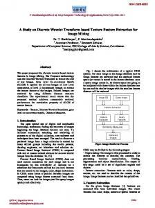
Where 𝑑 = denotes the dimension of the pattern vector 𝑥. 𝑖= pattern number, 𝑁= denotes the total number of samples in class, 𝑥𝑘𝑖 = vector of i-th training pattern from class 1, T= vector transpose. The σ is the "smoothing parameter" which represents the single free parameter for this algorithm [5],[6]. The architecture of PNN is shown figure 1.

660

image preprocessing techniques are playing significant role in MRI brain image, they perform the quality of an image and make it appropriate for the next step. The MRI brain image is enhanced with image enhancement techniques such as image filtering, in this proposed system type of filter is consider median filter, the results of median filter which gives good results.

4.2 IMPLEMENTATION 2D DISCRETE WAVELET TRANSFORM Decomposition the image is done utilizing Haar wavelet transform up to one level and two levels. Image of size (256 × 256) pixels yields four subimages each with size (128 × 128) pixels in first level. In the second level only the sub-image with "Low-Low" features will be decomposed to yield another four subimages each with size (64 × 64) pixels. Figure (3) represents one and two levels wavelet decomposition.

Figure (1): Architecture of PNN.

IJSER

4. PROPOSED SYSTEM

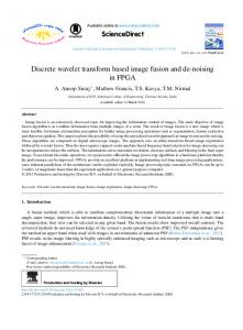
This work presents the proposed system started by presenting general block diagram of the natural and tumors type classification system. The programming language utilized to build the proposed system is MATLAB. The proposed system is suggested to be utilized as a tool for the radiologist and surgeon. This tool is to detect normal and tumors in MRI brain images and define tumors type shown in figure 3.

Figure (2): Block Diagram of the Normal and Tumors Type Classification System.

4.1 IMAGE PREPROCESSING In the proposed system deepened on MRI human brain images normal and six types of tumor are considered, these are Lymphoma, Glioblastoma multiform, Cystic oligodendroglioma, Ependymoma, Meningioma and Anaplastic astrocytoma. The numbers of collected images are 140 (20 images for each type of the six tumors and 20 image normal cases). In preprocessing image step the proposed system consists of multiple steps, they are, first step initially the input image is fed to the system, the input image may be a highly non stationary one, and hence convert the size of the input image to 256×256. In gray scale coding even if the input image is a color image it will be converted into gray scale image utilizing RGB converter and convert BMP, PNG to JPEG image (.jpg) file format. Second step enhance the medical MRI brain image utilizing median filter

(a)

(b)

(c)

Figure (3): DWT of MRI Tumors and Normal Brain Images, a. Original image, b. Image after the first level of decomposition, c. Image after the second level of decomposition.

4.3 FEATURE EXTRACTION

In pattern classification and in image processing, feature extraction is a special form of dimensionality reduction. When the input data to an algorithm is too large to be processed and it is suspected to be notoriously redundant (much data, but not much information) then the input data will be transformed into a reduced representation set of features. Transforming the input data into the set of features is named features extraction. Useful features of the image are extracted from the image for classification purpose [7],[8]. Statistical texture description methods define texture based on describing the spatial distribution of gray values. The simplest statistics are the gray level first-order statistics [7],[9]. For quantitatively describing the first order statistical (FOS) features of the image, useful features of the image can be obtained from the histogram. Mean is the average value of the intensity of the image. Average contrast is indicates the intensity variations around the mean [7],[10]. 𝑁𝑔 −1

𝑀𝑒𝑎𝑛 = 𝜇 = �

𝑖=0

𝑖 𝑃 (𝑖)

𝑁𝑔 −1

𝐴𝑣𝑒𝑟𝑎𝑔𝑒 𝐶𝑜𝑛𝑡𝑟𝑎𝑠𝑡 = 𝜎2 = �

𝑖=0

(4)

(𝑖 − 𝜇)2 𝑃(𝑖) (5)

And utilizing Gray-Level Co-occurrence Matrix (GLCM) describes the gray level of an image. Second-order statistics such as the co-occurrence matrices and the gray level difference method depict spatial relationships between image pixels [7],[9]. GLCM proposed by Haralick [10] has become one of the most

IJSER © 2016 http://www.ijser.org

International Journal of Scientific & Engineering Research, Volume 7, Issue 5, May-2016 ISSN 2229-5518

well-known and widely utilized texture measures. Energy: means uniformity, or Angular Second Moment (ASM), more homogeneous the image [11]. 𝑁𝑔 −1 2 (6) 𝐸𝑛𝑒𝑟𝑔𝑦 = ∑𝑖,𝑗=0 𝑃𝑑 (𝑖, 𝑗) Entropy: is a measure of randomness of intensity image [11]. 𝑁𝑔 −1

𝑃𝑑 (𝑖, 𝑗) 𝑙𝑜𝑔 (𝑃𝑑 (𝑖, 𝑗))

𝐸𝑛𝑡𝑟𝑜𝑝𝑦 = − �

𝑖,𝑗=0

(7)

Homogeneity: or Inverse Difference Moment (IDM) measures the similarity of pixels. A diagonal GLCM gives homogeneity of 1 [11]. 𝑁𝑔 −1 𝑃𝑑 (𝑖, 𝑗) (8) Homogeneity = � 1 + (𝑖, 𝑗)2 𝑖,𝑗=0 Maximum Probability: is determined the most prominent pixel pair in an image [12]. (9) Maximum Probability = max 𝑖, 𝑗 𝑃𝑑 (𝑖, 𝑗)

4.4 IMPLEMENTATION CLASSIFICATION SYSTEM

PROPOSED

When starting proposed system; the main interface of the system will appear on the screen, the main interface has two main phases (training and testing phases). In this work trained the probabilistic neural network with 105 MRI human brain images of data set where each images represents six tumors samples and normal sample for the testing phase. That means the proposed system has 105 trained samples stored in database. We compute six features extraction for six subimages from DWT. Hence the total feature extraction data length vector will be (105×36) for each subimages. PNN consists of four layers: 1. Input Layer: which consists of 36 nodes (length of each input vector). 2. Pattern Layer: which consists of 3780 hidden nodes (number of feature extraction vectors). Summation Layer: which consists of 7 hidden nodes (number of classes). 3. Output Layer: which consists of 1 node. Algorithm: Begin Step1: Read the input color medical MRI human brain images. Step2: Resize this image in to 256×256 image matrix. Step3: Converts the image from JPEG image (.jpg) file format to data file. Step4: Converts input color image in to grayscale image. Step5: Enhancement image utilizing median filter. Step6: Apply the Discrete Wavelet Transform Decompose the image into 2-D DWT with two levels, segmentation image into 7 subimages, starting from the top left corner, (L2 L2 , L1 H 1 , H 1 L1 , H 1 H 1 , L2 H 2 , H 2 H 2 , and H 2 L2 ). Step7: Compute the normalized utilizing of first order statics (FOS) mean utilizing equation (5), average contrast utilizing equation (4) and second order statics (Gray Level Co-occurrence Matrix) (CLCM) with d=1 for distance and 𝜃 = 0 degrees, energy utilizing equation (6), entropy utilizing (7), homogeneity equation (8), max probability utilizing (9) for each subimages except the one with "lowlow" subimage (L2 L2 ).

661

Step8: Save the normalized mean, average contrast, energy, entropy, homogeneity, and maximum probability in the feature extraction file DB. Step9: Build the PNN and load the feature extraction data (DB) to train the neural network. Step10: Input the results from steps (6 and 7) to the neural network. 10.1 Find the estimated PDF for each hidden node in pattern layer. 10.2 Find the sum of each node in summation layer) summation of estimated PDF for each class). 10.3 Find the probability of each class by divided the sum of estimated PDF for each class over the sum of all estimated PDF. 10.4 Find the reference in feature extraction file. Step11: Assign the unknown image to class with probability largest. End

4. EXAMPLE OF CLASSIFICATION ALGORITHM OR PHASE)

IMPLEMENTING PROPOSED DWT (TESTING

IJSER

R

R

R

R

R

R

R

R

R

R

R

R

R

R

R

R

R

R

R

R

R

R

R

R

R

R

R

R

R

R

R

To improve the correctness of the algorithm, let us take an example to demonstrate the application of the classification algorithm. The example is: Step1: Read medical color MRI brain image (TestImage/.Lymphoma). Step2: Resize this image in to 256×256 image matrix. Step3: Converts the image from JPEG image (.jpg) file format to data file. Step4: Converts input color image in to grayscale image. Step5: Enhancement image utilizing median filter. Step6: Decompose the image into 2-D DWT with two levels to get subimages. Step7: The normalized mean, average contrast, energy, entropy, homogeneity, and maximum probability values of the 6 subimages are: Sub images

Homogeneity

Energy

Entropy

Average Contrast

mean

Maximum Probability

H1 L1 L1 H1 H1H1 H2 L2 L2 H2 H2H2

551 100 250 28 424 59

1.1776 1.0132 8.7875 3.4599 3.1632 2.7032

1.3506 1.3467 1.4235 1.4166 1.4130 1.5871

8.4783 7.8641 2.3159 29.0674 27.7931 8.1248

0.0336 0.0061 0.0152 0.0068 0.1035 0.0143

54 70 30 159 182 86

R

R

R

R

R

R

R

R

R

R

R

R

R

R

R

R

R

R

Step8: Build the Probabilistic Neural Network. Step9: Load the feature extraction data to train the neural network. Step10: Input the results from step (7) to the neural network. 10.1: The estimated PDF for each hidden node in pattern layer are:

R

IJSER © 2016 http://www.ijser.org

International Journal of Scientific & Engineering Research, Volume 7, Issue 5, May-2016 ISSN 2229-5518 1.5574 2.0940 1.9948 1.0142 2.8876 1.4776 1.6893 1.4422 1.4359 1.1536 1.4206 1.1360 1.6173 1.1168

1.1488 0.8183 2.0275 2.1279 1.6534 1.9253 1.2283 2.1290 0.8723 1.6615 1.8955 2.4075 1.1960 ---

1.0092 1.1545 1.1215 1.1296 1.1547 1.1419 0.9891 1.1620 1.0630 1.2658 0.9896 1.4729 0.9900 ---

1.1594 1.2446 1.0543 0.9354 1.3615 0.9616 1.1326 1.2206 1.6092 1.1558 1.3175 1.3735 1.0488 ---

1.7875 1.3717 0.9771 1.4123 1.4783 3.7349 1.1592 1.1301 1.5307 1.6615 0.8985 1.1799 1.2842 ---

1.3919 0.9877 0.8363 2.3589 1.0885 1.4284 0.9196 1.0751 0.9140 2.0954 1.1741 1.5720 1.0927 ---

0.8441 1.4464 1.4200 2.0750 1.2004 0.8787 1.4807 0.9685 1.0079 1.3454 1.2073 1.0726 1.0364 ---

0.8643 1.4738 1.1005 1.4889 1.0900 1.2446 1.1212 1.3210 1.0725 0.9059 1.3740 0.9378 1.0908 ---

10.2: The summation of each node in summation layer (summation of estimated PDF for each class) are: Sum 1

Sum 2

Sum 3

Sum 4

Sum 5

Sum 6

Sum 7

23.3631

18.5702

20.9810

21.4834

21.4834

21.4834

21.4834

R

R

R

R

R

R

R

The total summation =140.9601 10.3: The probability of each class by dividing the summation of estimated PDF for each class over the summation of all estimated PDF are: P1 0.1657 R

P2 0.1317 R

P3 0.1488 R

P4 0.1524 R

P5 0.1308 R

P6 0.1432 R

P7 0.1273 R

Step11: Assign the unknown image to a class that is fired from PNN (with largest probability) (Class = Lymphoma) Step12: End.

International Conference on Information Science, Signal Processing and their Applications (ISSPA), IEEE, 2010. 6. K.Z. Mao, K.-C. Tan, and W. Ser, "Probabilistic NeuralNetwork Structure Determination for Pattern Classification", IEEE Transactions on Neural Networks, Vol. 11, No. 4, July 2000. 7. Qurat-Ul-Ain, G. Latif, S. Batool Kazmi, M. Arfan Jaffar, and A.M. Mirza, "Classification and Segmentation of Brain Tumor using Texture Analysis", proceedings of the 9th WSEAS International Conference on Artificial Intelligence, Knowledge Engineering and Databases (AIKED), pp. 147-155, 2010. 8. M. Arora, "Detection of Abnormalities in MRI Images using Texture Analysis", M.SC. Thesis, college of Engineering in Electronics Instrumentation and Control, ELECTRICAL AND INSTRUMENTATION ENGINEERING DEPARTMENT THAPAR UNIVERSITY, Thapar University, Patiala, JUNE 2009. 9. N. Nabizadeh, M. Kubat, "Brain tumors detection and segmentation in MR images: Gabor wavelet vs. statistical features", Computers and Electrical Engineering xxx (2015) xxx–xxx, pp.1-15, FEBRUARY 2015. 10. R. M. Haralick and K. Shanmugam., "Textural feature for image classification", IEEE Transactions on Systems, Man, And Cybernetics, SMC–3(6):610–619, November 1980. 11. N. Bian, "Evaluation of Texture Features for Analysis of Ovarian Follicular Development", M.SC. Thesis, college of Science in the Department of Computer Science University of Saskatchewan Saskatoon, Canada, December 2005. 12. A. Gebejes and R. Huertas, "Texture Characterization based on Grey-Level Co-occurrence Matrix", Conference of Informatics and Management Sciences, pp.375-378, 25 – 29 March 2013.

IJSER

6. RESULTS AND CONCLUSIONS

The importance of this work is improving a neural network training method utilized for building a program for MRI human brain diagnosis that may help physician in their diagnosis. The algorithm is applied on 35 MRI brain images from different types will be utilized as testing data phase. The result represents that 32 images are classified correctly and the other 3 images are not classified correctly. The system classification proved its effectiveness to classify MRI brain normal and tumors type. The percentage of accuracy of classification Utilizing PNN is found to be nearly 91 %. The PNN gives the system more power because it needs very short time for training and representing a good accuracy classifier. The proposed system may be applied for classified other cancers like breast cancer.

7. REFERNCES 1.

2. 3. 4.

5.

662

P. John, "Brain Tumor Classification Using Wavelet and Texture Based Neural Network", International Journal of Scientific & Engineering Research Volume 3, Issue 10, ISSN 2229-5518, pp. 1-7, October 2012. R. Nikhil, "Speech Compression Using Wavelets", M.Sc. Thesis, University of Queensland, October 2001. D. F. Specht., "Probabilistic Neural Networks", Neural Networks, vol. 3, no. 1, pp. 109-118, 1990. P. MUTHUKRISHNAMMAL, S. SELVAKUMAR R., "CLUSTERING AND NEURAL NETWORK APPROACHES FOR AUTOMATED SEGMENTATION AND CLASSIFICATION OF MRI BRAIN IMAGES", Journal of Theoretical and Applied Information Technology, Vol.72 No.3, pp. 322-330, 28th February 2015. S. Meshoul and M. Batouche, "Combining Fisher Discriminant Analysis and Probabilistic Neural Network for Effective On-Line Signature Recognition", 10th

IJSER © 2016 http://www.ijser.org