Brain-inspired Recurrent Neural Algorithms for ... - Kreiman Lab

WEBSTYLEGUIDE

Institute for Software & Systems Engineering Universitätsstraße 6a

D-86135 Augsburg

Brain-inspired Recurrent Neural Algorithms for Advanced Object Recognition Martin Schrimpf

Master’s Thesis in the Elite Graduate Program Software Engineering

WEBSTYLEGUIDE

Institute for Software & Systems Engineering Universitätsstraße 6a

D-86135 Augsburg

Brain-inspired Recurrent Neural Algorithms for Advanced Object Recognition Student id: Start date: End date: Primary reviewer: Secondary reviewer: Advisor:

1400809 07. 09. 2016 13. 05. 2017 Prof. Dr. Alexander Knapp Prof. Dr. Elisabeth André Prof. Dr. Alexander Knapp

DECLARATION

I confirm that this thesis is my own work and that I have documented all sources and material used.

Dorfen, 15. 05. 2017

Martin Schrimpf

Contents

1. Introduction

1

2. Advances in Deep Learning

5

2.1. Computer Vision . . . . . . . . . . . . . . . . . . . . . . . . . . . . . . . . . . . . . . . . .

5

2.2. Natural Language Processing . . . . . . . . . . . . . . . . . . . . . . . . . . . . . . . . . .

7

2.3. Deep Reinforcement Learning . . . . . . . . . . . . . . . . . . . . . . . . . . . . . . . . . .

8

2.4. Applications . . . . . . . . . . . . . . . . . . . . . . . . . . . . . . . . . . . . . . . . . . . .

9

3. Building Blocks of Deep Neural Networks

11

3.1. Basic Network Formulation . . . . . . . . . . . . . . . . . . . . . . . . . . . . . . . . . . . 11 3.1.1. Activity of a Single Layer . . . . . . . . . . . . . . . . . . . . . . . . . . . . . . . . 11 3.1.2. Objective Functions . . . . . . . . . . . . . . . . . . . . . . . . . . . . . . . . . . . 12 3.1.3. Weight Initialization . . . . . . . . . . . . . . . . . . . . . . . . . . . . . . . . . . . 12 3.1.4. Backpropagation . . . . . . . . . . . . . . . . . . . . . . . . . . . . . . . . . . . . . 12 3.1.5. Stacking Layers . . . . . . . . . . . . . . . . . . . . . . . . . . . . . . . . . . . . . . 13 3.1.6. Fine-Tuning . . . . . . . . . . . . . . . . . . . . . . . . . . . . . . . . . . . . . . . . 13 3.2. Fully-Connected Layers . . . . . . . . . . . . . . . . . . . . . . . . . . . . . . . . . . . . . 14 3.3. Convolutional Layers . . . . . . . . . . . . . . . . . . . . . . . . . . . . . . . . . . . . . . . 14 3.4. Pooling Layers . . . . . . . . . . . . . . . . . . . . . . . . . . . . . . . . . . . . . . . . . . 15 3.5. Recurrent Layers . . . . . . . . . . . . . . . . . . . . . . . . . . . . . . . . . . . . . . . . . 16 3.6. Hopfield Networks . . . . . . . . . . . . . . . . . . . . . . . . . . . . . . . . . . . . . . . . 17 4. Object Recognition in the Brain

21

4.1. The Brain . . . . . . . . . . . . . . . . . . . . . . . . . . . . . . . . . . . . . . . . . . . . . 21 4.2. Visual Cortex . . . . . . . . . . . . . . . . . . . . . . . . . . . . . . . . . . . . . . . . . . . 23 5. Applied Neural Networks

27

5.1. Artificial Neural Networks in Computer Vision . . . . . . . . . . . . . . . . . . . . . . . . 27 5.1.1. HMAX . . . . . . . . . . . . . . . . . . . . . . . . . . . . . . . . . . . . . . . . . . 27 5.1.2. Alexnet . . . . . . . . . . . . . . . . . . . . . . . . . . . . . . . . . . . . . . . . . . 27 5.1.3. VGG . . . . . . . . . . . . . . . . . . . . . . . . . . . . . . . . . . . . . . . . . . . . 29 5.1.4. Inception . . . . . . . . . . . . . . . . . . . . . . . . . . . . . . . . . . . . . . . . . 29 5.1.5. Residual Networks . . . . . . . . . . . . . . . . . . . . . . . . . . . . . . . . . . . . 31 5.1.6. General Approach of Today’s Computer Vision Networks . . . . . . . . . . . . . . 32 5.2. Current Applications of Recurrent Neural Networks . . . . . . . . . . . . . . . . . . . . . 32

i

Contents 6. Recurrent Computations for Partial Object Completion

35

6.1. Robust Human Recognition of Partial Objects . . . . . . . . . . . . . . . . . . . . . . . . . 36 6.1.1. Backward Masking Interrupts Recurrent Computations . . . . . . . . . . . . . . . 37 6.1.2. Similar Effects in Object Identification . . . . . . . . . . . . . . . . . . . . . . . . . 38 6.1.3. Neurophysiological Delays when Recognizing Partial Objects . . . . . . . . . . . . 39 6.2. Feed-Forward Networks Are Not Robust to Occlusion . . . . . . . . . . . . . . . . . . . . 39 6.2.1. Feature Representations Are Hard to Separate . . . . . . . . . . . . . . . . . . . . 41 6.2.2. Correlation Between Model Feature Distance and Neural Response Latency . . . . 41 6.3. Robust Computational Recognition of Occluded Objects with Attractor Dynamics . . . . 42 6.3.1. Recurrent Hopfield Model with Whole Representations as Attractors . . . . . . . . 43 6.3.2. Recurrent Models Trained to Minimize Distance Between Partial and Whole Representations . . . . . . . . . . . . . . . . . . . . . . . . . . . . . . . . . . . . . . . . 43 6.3.3. Recurrent Models Approach Human Performance on Partial Objects . . . . . . . . 44 6.3.4. Recurrent Models Approach Human Performance on Partial Objects . . . . . . . . 46 6.3.5. Recurrent Models Increase Correlation with Human Behavior . . . . . . . . . . . . 48 6.3.6. Recurrent Models Capture the Effects of Backward Masking . . . . . . . . . . . . . 49 6.4. Discussion . . . . . . . . . . . . . . . . . . . . . . . . . . . . . . . . . . . . . . . . . . . . . 49 7. Increasing Object Likelihoods by Integrating Visual Context

53

7.1. Empirical Proof of Existence of Context Utilization in Human Behavior . . . . . . . . . . 53 7.1.1. Dataset of Hand-Picked Context Images . . . . . . . . . . . . . . . . . . . . . . . . 53 7.1.2. Labeling Through Mturk . . . . . . . . . . . . . . . . . . . . . . . . . . . . . . . . 53 7.1.3. Significant Performance Deficits Without Visual Context . . . . . . . . . . . . . . 54 7.1.4. Context Allows for More Educated Guesses . . . . . . . . . . . . . . . . . . . . . . 56 7.1.5. Backward Masking Disrupts Objects in Isolation and with Context Equally . . . . 57 7.2. Feed-Forward Alexnet Does Not Make Significant Gains with Context . . . . . . . . . . . 59 7.3. Recurrency as a Way of Integrating Context Information . . . . . . . . . . . . . . . . . . . 60 7.3.1. A Simple Recurrent Model of High-Level Information Integration . . . . . . . . . . 60 7.3.2. Incorporating Semantic World Information to Utilize Context . . . . . . . . . . . . 61 7.4. Discussion . . . . . . . . . . . . . . . . . . . . . . . . . . . . . . . . . . . . . . . . . . . . . 63 8. Conclusion

65

Appendix A. Complete Data for Recurrent Computations for Partial Object Completion

69

List of Figures

73

List of Tables

75

References

77

ii

Acknowledgements

I am extremely grateful for the opportunities and tremendous support given to me by Prof. Dr. Gabriel Kreiman at Boston Children’s Hospital, Harvard Medical School. I could always count on him for discussions and never left his office without a fruitful discussion and a page full of exciting questions. His guidance boosted my skills as an independent researcher significantly and allowed me to thrive in a challenging environment. I would also like to thank the whole group at the Kreiman lab, in particular the individuals I cooperated with in the course of this Thesis: Bill Lotter and Hanlin Tang from Harvard Biophysics on partial object completion, Wendy Fernández from the City University of New York on the identification of partially occluded objects, and Jacklyn Sarette from Emmanuel College on the human psychophysics of visual context. In this regard, I would also like to thank the participants of our human studies. Thank you as well to the administrators, faculty and researchers at the Center for Brains, Minds and Machines that allowed me to gain broad and deep insights into the current research in machine learning as well as brain and cognitive science with the many workshops and courses offered by the center. I am thankful to Prof. Dr. Alexander Knapp at the University of Augsburg for his support on writing this Thesis and the productive discussions on this work as well as throughout my Master’s. Finally, I would like to thank my family for the unfailing support and continuous encouragement.

Abstract

Deep learning has enabled breakthroughs in machine learning, resulting in performance levels seeming on par with humans. This is particularly the case in computer vision where models can learn to classify objects in the images of a dataset. These datasets however often feature perfect information, whereas objects in the real world are frequently cluttered with other objects and thereby occluded. In this thesis, we argue for the usefulness of recurrency for solving these questions of partial information and visual context. First, we show that humans robustly recognize partial objects even at low visibilities while today’s feed-forward models in computer vision are not robust to occlusion with classification performance lacking far behind human baseline. We argue that recurrent computations in the visual cortex are the crucial piece, evident through performance deficits with backward masking and neurophysiological delays for partial images. By extending the neural network Alexnet with recurrent connections at the last feature layer, we are able to outperform feed-forward models and even human subjects. These recurrent models also correlate with human behavior and capture the effects of backward masking. Second, we empirically demonstrate that human subjects benefit from visual context in recognizing difficult images. Building on top of feed-forward Alexnet, we add scene information and recurrent connections to the object prediction layer to define a simple model capable of context integration. Through the use of semantic relationships between objects and scenes derived from a lexical corpus, we can define the recurrent weights without training on large image datasets. The results of this work suggest that recurrent connections are a powerful tool for integrating spatiotemporal information, allowing for the robust recognition of even complex images.

CHAPTER

1

Introduction

Intelligent algorithms - whether biological or in silicon - must often make sense of an incomplete and complex world. Inference and integration of information therein allow to draw the most likely conclusions from a set of premises and are essential for intelligent algorithms to operate in an ambiguous environment. In vision, objects are almost never isolated in the real world; rather, they are partly hidden behind other objects and related to the objects around them. While other fields of artificial intelligence are already partly able to infer information, approaches in computer vision typically do not perform sophisticated inference. And although we know of the existence of recurrent connections in the visual cortex from neuroanatomy, neither is it well understood what role they play in object recognition nor do any of the state-of-the-art computer vision architectures feature recurrency. We will examine here the usefulness of recurrent connections in performing inference and integration in visual object recognition. Recent advances in artificial intelligence often stem from deep learning which uses neural networks with multiple layers of neurons. These models are capable of learning a multitude of tasks without requiring hand-crafted rules or features. Historically, assigning credit [93] to individual units and thereby allowing the network to learn has already been discussed back in 1974 with an algorithm that propagated deviations between predictions and ground truths back through the network [141]. Neural networks with multiple layers were then further popularized when the emergence of useful internal representations in the hidden layers was demonstrated [115, 118]. On vision datasets [26, 34, 66, 73, 82, 116], deep convolutional neural networks [36, 67, 125, 134, 151] now achieve performance-levels comparable to humans [36]. Tremendous progress has also been made in Natural Language Processing where deep models learn internal representations that enable them to achieve superior performances across a number of tasks [18, 55, 69, 92, 127, 132] and in reinforcement learning where actors can be trained end-to-end to play a variety of games [80, 95, 96, 124] or even learn the model itself [3, 23]. Deep learning is increasingly gaining traction in a broad range of domains and numerous real-world applications already exist, including the reconstruction of brain circuits [39], the analysis of particle accelerator data [2] and skin cancer classification [25]. Originally inspired by neuroscience [50, 110], artificial neural networks have since predominantly been guided by mathematical optimization [131] rather than the structure of the brain [89]. Despite this divergence of neuroscience and machine learning, neural networks are highly correlated with and predictive of neural activity [148], and especially the rapid object recognition occurring in the first few hundred milliseconds of visual processing is described with increasing level of detail [19, 21, 86, 110, 111, 120,

1

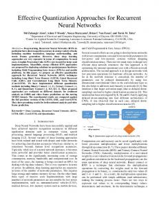
1. Introduction 135]. From a neuroanatomy point of view however, feed-forward networks represent only a subset of the connections found in visual cortex considering that the brain is recurrent and contains feedback as well as horizontal connections [29, 71, 84]. The effects of these recurrent signals are often minimized in vision experiments by backward masking [9, 24, 62, 65, 70, 112, 120, 140]. While recurrent neural networks are used widely in other fields like natural language processing, computer vision heavily relies on feed-forward architectures at this point in time. These models have yielded convincing results but, as we show later, fail to perform tasks requiring inference and integration. Similarly, the visual cortex in the brain is thought to contain not only feed-forward connections but also recurrent connections, i.e. horizontal and feedback loops. This thesis discovers the usefulness of recurrent connections to applications in computer vision: the recognition of occluded objects and the utilization of context. In particular, while deep convolutional networks achieved breakthroughs in computer vision with invariance to scale and rotation of the objects [72], the relevant datasets largely contain images in good conditions with little clutter or blurring and objects are isolated or at least roughly centered in the image without being occluded by other objects or ambiguity. The real world however is usually very different: scenes of objects are complex with objects not appearing in isolation but rather with dozens of other objects and due to the three-dimensionality of our world, objects appear behind one another which leads to occlusions. Consider Figure 1.1 for instance - how many of the objects in the image are perfectly visible, without any distortions? And while the brain has a remarkable ability to recognize objects from

Figure 1.1.: The real world: a street scene in New York City only minimal information (you can probably still recognize almost all of the objects in Figure 1.1), artificial feed-forward networks struggle with occlusion (Section 6.2). As humans, we can also use information about the scene and other objects to make an educated guess about the identity of an object, even if it is barely visible at all or could be interpreted as a number of things (ambiguity). As a way of integrating spatial information in a brain-like manner, we propose the incorporation of recurrent connections into computer vision architectures. We show their usefulness for the recognition of occluded objects where recurrency can be used to define attractor-mechanics and for the utilization of visual context where they can integrate surrounding scene and object information to increase the likelihood of the most probable object.

2

Chapter 2 highlights recent advances in the core fields of deep learning, which Chapter 3 examines closer by describing the building blocks relevant for computer vision. Chapter 4 gives a neuroscientific overview over the building blocks thought of making up the brain (Section 4.1) and goes into more detail about the current understanding of how the visual cortex performs basic object recognition (Section 4.2). Chapter 5 analyzes applied neural networks in current object recognition models (Section 5.1) and the present applications of recurrency in other domains (Section 5.2). The next two chapters then focus on our proposed models to demonstrate the usefulness of recurrency in deep learning networks for computer vision: Chapter 6 shows evidence for recurrent connections in the visual cortex of humans (Section 6.1) and evaluates how well low visibilities in images can be handled by current feed-forward models (Section 6.2) and by a proof-of-concept network incorporating recurrency (Section 6.3). Chapter 7 describes our findings of humans psychophysics for objects in isolation and with visual context (Section 7.1), examines the same task in a state-of-the-art feed-forward model (Section 7.2) and analyzes a simple model that can integrate high-level visual information through semantic relationships (Section 7.3). Finally, Chapter 8 concludes the work with a summary and discussion about the feasibility of our approaches as well as future directions for recurrent architectures in computer vision.

3

CHAPTER

2

Advances in Deep Learning

The field of deep learning has made tremendous progress in recent years, achieving breakthroughs in a range of domains with a vast number of real-world applications. Training these deep neural networks with millions of parameters1 is made possible by today’s cheap, increasingly powerful and parallel GPUs which excel at the fast matrix and vector multiplications required for computations in these networks [118]. There have also been first theoretical insights into the ability of deep and not shallow networks to compose functions [105] and their relation to physics which lay constraints on e.g. the variety of images that can occur naturally [81]. In addition, a quick implementation of ideas and concepts is enabled by machine learning frameworks [119] such as TensorFlow [1], Theano [109], keras [14], Caffe [53], Torch [17], CNTK [149], MXNet [12] or pytorch2 . The core fields of deep learning - computer vision, natural language processing and reinforcement learning - have seen great improvements just like neural networks have spread out to learn about many other domains.

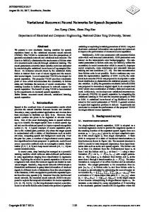
2.1. Computer Vision With the introduction of stacked (deep) convolutional layers in networks that could learn image features end-to-end in 1998, a new era of deep learning for vision had been started [74]. Challenges that provide massive labeled datasets with up to millions of images include MNIST [73] (70k images of handwritten digits, 10 categories), Pascal VOC [26] (1578 images of real-world objects and 4 categories in 2005, 12k images and 20 categories at the end of the challenge in 2012), CIFAR [66] (60k object images, 10 or 100 categories), ImageNet (3.2 million object images in 2009 [52], 14.2 million images in 2014 [116], 1000 categories, see Figure 2.1 for examples), Caltech-256 [34] (31k object images, 256 categories) and COCO [82] (2.5 million labeled instances in 328k images of scenes). These datasetes allow the models to learn many different image aspects and thereby generalize well to new images. As a result, performance of deep neural networks approaches or even surpasses human performance levels [36] on these narrow tasks. Winners of the yearly Imagenet challenge include the popular deep convolutional networks listed in Table 2.1 along with their depth, i.e. the number of layers. A clear trend is to increase the number of layers which generally leads to increased recognition performance when taking care of obstacles like vanishing gradients and degradation (Section 5.1 and Chapter 3). Note that the error rates are top5 errors, meaning that the network can “guess” 5 labels and if one of them is correct, the answer is 1A

recent mixture-of-experts approach even uses up to 137 billion parameters [123]

2 http://pytorch.org/

5

2. Advances in Deep Learning

Figure 2.1.: Examples of images and their labels in ImageNet [52] Year 2012 2013 2014 2015

Network Alexnet ZF Net GoogLeNet ResNet

layers 8 8 22 152

top-5 error 16.4% 11.7% 6.7% 3.6%

Table 2.1.: Popular network architectures along with the number of layers and their top-5 object classification error rates on the respective ImageNet test set [116]

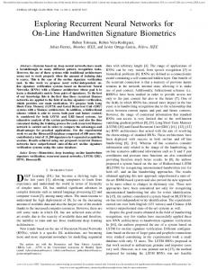
considered correct. This is done to combat the occurrence of multiple objects in the same image. For comparison, the best results on ImageNet before Alexnet were achieved with hand-crafted algorithms for feature extraction (SIFT and Fisher-Vectors) [117] and achieved top-5 errors of 25.8% - Alexnet almost halved these error rates [67]. In addition, the competing models from the table often show the performance of network-ensembles which typically achieve better results than a single network (think of multiple human experts). The winner of ILSVRC 2016 used such an ensemble of several previously proposed models and achieved a 3.0% top-5 error3 . Most of the networks so far rely heavily on the availability of huge labeled datasets and are largely trained in a supervised manner (although potentially aided by unsupervised pre-training [45]). This reliance on manual labels places a constraint on learning and as a result, unsupervised learning is becoming more and more important. One such recent approach is that of Generative Adverserial Networks (GANs) [31] which replaces the label-optimization on a defined cost-function with a trainable network. Training the network is done in a minimax game where the generator creates images from a latent space and the discriminator distinguishes between these synthesized images and real ones, ultimately enabling the creation of realistically looking images. By combining this approach with natural language processing (Section 2.2), one can condition the GAN on the caption and create images corresponding to the given text [49, 152]. Although these generated images illustrated in Figure 2.2 are not perfect, they are better than anything

Figure 2.2.: Examples of images generated from language [152] 3 http://image-net.org/challenges/LSVRC/2016/results#loc

6

2.2. Natural Language Processing before and will likely be refined more and more to enable the generation of realistic data distributions. An earlier approach is that of autoencoders [138], and recently variational autoencoders [63], which basically reconstruct their input. However, they do so within a network that maps from input to a small number of hidden neurons to output so the model has to find a good representation of the data to minimize the reconstruction error. The assumption here (and in any deep learning architecture with a decrease in the number of neurons for each layer) is that such a minimal representation exists which seems to be supported by the laws physics limiting the possible combinatory explosion of pixel values in an image [81]. Unsupervised learning can also be realized by ideas of predictive coding drawn from neuroscientific findings [108]: a deep recurrent convolutional neural network can be trained to predict future frames in a video sequence and will learn internal representations that are useful for object recognition without relying on many labeled examples [87].

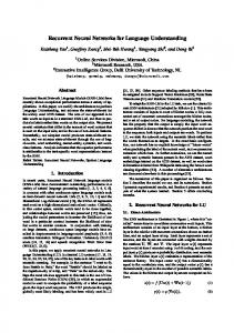
2.2. Natural Language Processing Deep learning has not only empowered object recognition, but also significant advances have been made in natural language processing (NLP): while sentences were traditionally represented with sparse bag-ofwords [35], more recent deep learning approaches use distributed, learned representations of increasing abstraction [127, 132]. Architecture-wise, recursive neural networks are used which allow to incorporate the intrinsic compositionality of the human language, composed of words and phrases, into the models. With a defined architecture and input-output pairs, these networks can then be trained end-to-end and achieve superior performance compared to previous hand-crafted models. For instance, by comparing different NLP models on datasets such as the Penn Treebank [90], measuring the perplexity to new words, it has been shown that recurrent neural network models combined with standard n-gram models alone achieve performance levels that make it mostly unnecessary to use further techniques [92]. Crucially, utilizing internal representations learned by deep neural networks, the model can be re-used for a number of tasks, such as “part-of-speech tagging, chunking, named entity recognition, and semantic role labeling” [18]. As an example of the usefulness of these rich, learned representations, consider an extension of Google’s Neural Machine Translation system (GNMT) which can translate between multiple languages [55]. While it produces state-of-the-art results on translation benchmarks for the languages it has been trained on, such as Japanese ⇔ English and Korean ⇔ English, it shares its parameters for any translation-pair and can thus transfer this knowledge to other pairs. This shared internal representation allows the model to translate between language pairs it has never seen before, such as Korean ⇔ Japanese, a convincing demonstration of transfer learning termed “zero-shot translation”. Similar to the previous combination of GANs in computer vision and NLP, we can also go from vision to language by captioning images. In [147], this is done by producing sentences with a recurrent neural network that uses the features of a deep convolutional neural network (see Figure 2.3). The network can be trained end-to-end and learns to attend to parts of the image while generating the caption. Moreover, combining the dynamic memory network [69] with an object recognition model enables it to answer questions for input images by using an attention mechanism and ideas from episodic memory [146] (see Figure 2.4).

7

2. Advances in Deep Learning

Figure 2.3.: Examples of captions generated from images [147]

Figure 2.4.: Visual question answering for different input image-question pairs [146]

2.3. Deep Reinforcement Learning

Reinforcement learning (RL) aims to solve a sequential decision making problem - such as playing Atari games [95] - by maximizing the long term rewards from the environment. To decide which action to take in a certain state, the agent follows a policy that outputs an action for any given state. In some cases, this policy uses a function that predicts future rewards: the action-value function Q computes the expected return for an action in a state and consecutive policy behavior and the function V gives us the predicted value of a state. Based on these components, different learning algorithms can be applied. Value-based methods like temporal difference learning (TD) and Q-learning learn the value function V or the action value function Q respectively - the policy is then derived from the optimal value function. In contrast, policy-based methods optimize the policy directly: REINFORCE updates the function’s parameters in the direction of the expected overall reward R for the policy whereas in actor-critic-algorithms, the action-value function is updated by the critic to direct the actor’s policy updates [78]. RL becomes deep RL when deep neural networks are used to compute any of components of the model, making the aforementioned function parameters the weights of a neural network. For instance, the deep Q-network [96] uses a network architecture of two convolutional and two fully-connected layers to learn the Q function. In policy-based approaches, deep networks are used to model the policy and in actorcritic-algorithms, a neural network can be used to express both parts [80]. Another recent success of deep RL was the win of AlphaGo over the Go world champion, with Go being “the most challenging of classic games for artificial intelligence” [124]. AlphaGo uses deep neural networks for the value function as well as the policy with multiple convolutions over the board position. Recent ideas include the differentiable neural computer [33] which enables long-term storage with a readwrite memory and learning-to-learn or meta-learning where the (often recurrent) model itself is learned by the algorithm instead of being crafted by hand [3, 23].

8

2.4. Applications

2.4. Applications Aside from the core fields of deep learning, a lot of progress is made in a range of other fields as well. The commercial world for instance is quickly changed by neural networks: brain circuits are reconstructed by training a feed-forward convolutional network to classify connectedness between voxels [39]; Google Translate is now implemented as a deep LSTM network instead of the previous phrase-based approach [145]; search results are guided by smart learning systems [16]; in finance, neural networks predict future stock prices [8]; job candidates can be automatically filtered based on their CVs [27]; machine learning techniques are used to find the optimal compression [113], leading to “up to 75 percent less bandwidth per image” 4 ; European banks use them to increase cash collections [106]; particle accelerator data can be analyzed with an ensemble of deep neural networks [2]; and skin lesions can be classified using a convolutional neural network, trained end to end [25]. Combining techniques from different domains shows successful in LipNet which is capable of “decoding text from the movement of a speaker’s mouth” [4] just like using deep learning models in new domains is gaining traction, e.g. in databases to predict future workloads [103].

4 https://www.blog.google/products/google-plus/saving-you-bandwidth-through-machine-learning/

9

CHAPTER

3

Building Blocks of Deep Neural Networks

Artificial neural networks can be composed by a combination of different concepts and techniques. By plugging these building blocks together, we create deep neural networks to perform a variety of tasks. While most of the following concepts are used across domains, the core focus will be on techniques in computer vision. The hyper-parameter formulation of these networks in terms of learning rules and architectures is typically done manually1 and thus different from the actual parameters of the network which are learned to fit the data. Datasets are generally split into a training, validation and test set. The model is then trained to minimize the error on the training set while the validation error measures generalization during training. Performance is ultimately measured on the previously unseen test set.

3.1. Basic Network Formulation Before stacking multiple layers to create deep neural networks, we first have to define a single layer and some basic techniques which are relevant across the whole network.

3.1.1. Activity of a Single Layer At the basic level of a network is the activity h of a single layer which is determined by its input vector x, the weight vector w (including a bias term) and the activation function f : h = f (wx) = f (

X

w i xi )

(3.1)

i

If h is the output layer, the activity of h is equal to the output vector y of the network. Activation functions f include the rectified linear unit (ReLU) [99] as well as sigmoid and tanh (Figure 3.1). In the output layer of a network applied to classification tasks, the softmax function is commonly used to relativize the output values to class probabilities that sum up to 1. Activation function can also be seen as their own layer but in this work, we will consider it to be part of one layer performing the whole task of combining the input with the weights and applying an activation function as described in Equation 3.1. 1 Notably,

new approaches in meta-learning are trying to get rid of the manual input of hyper-parameters

11

3. Building Blocks of Deep Neural Networks

3

sigmoid

tanh

3

2

2

2

1

1

1

0

0

0

-1

-1

-1

-2

-2

-2

-3 -5

0

5

-3 -5

ReLU

3

0

5

-3 -5

0

5

Figure 3.1.: Sample activation functions: while sigmoid and the hyperbolic tangent (tanh) scale their input to the range [0, 1] and [−1, +1] respectively, the rectified linear unit (ReLU) only sets negative inputs to zero (ReLU(x) = max(0, x)). However, the non-linearity introduced by the ReLU has proven to be very effective in practice

3.1.2. Objective Functions To denote how far off the prediction vector y is from the target vector yˆ, we then define an objective function that typically computes a scalar loss L, for instance the L1 loss or the L2 loss (also called mean-squared-error or MSE). L1 =

X

|yi − yˆi |

L2 =

i

X (y − yˆ)2 i

3.1.3. Weight Initialization Before training the network, weights are set to initial values. If data is properly initialized, a reasonable assumption is that the number of positive and negative weights will even out. Weights should however not be set to zero since every neuron would then compute the same output, thus the same gradient, and parameters would not differ among one another. Instead, weights are commonly initialized to small random values which breaks the symmetry between weights but keeps them close to zero [60]. A weight vector for a single neuron is commonly drawn from a Gaussian and the variance is scaled relative to the number of input units n [37]: r w = random(n) ×

2 n

where random(n) samples n values from a standard Gaussian and the term

q

2 n

scales the variance with

respect to ReLU activation functions.

3.1.4. Backpropagation To minimize our objective function, we use optimizers that improve the weights W of our network over time based on the inputs X, network predictions Y and a learning rate µ using the current (approximated) gradient of the network ∇W LW (Xi , Yi ) for an input-output pair (Xi , Yi ) [114]. Intuitively, we propagate errors back through the network (“backpropagation” [115, 141]) which can be done by applying stochastic gradient descent (SGD) to the weights: W = W − µ∇W LW (Xi , Yi )

12

3.1. Basic Network Formulation

Figure 3.2.: A three-layer network architecture2 : The weight vectors w1 , w2 , w3 are learned to fit outputs y for inputs x

Typically, variants of SGD like batch gradient descent or mini-batch gradient descent are used which handle batches of multiple inputs and outputs at once. This speeds up computations by using big matrix multiplications which GPUs can compute very quickly [118]. These variants of gradient descent are realized with different optimization algorithms; some common implementations are RMSprop, Adagrad and Adam. One can also add momentum to the descent of SGD which accelerates convergence in the direction of the dimensions where the gradients point in the same direction [114].

3.1.5. Stacking Layers By combining multiple layers, the output of a lower layer becomes the input of the layer one level above, thus chaining the respective functions. The output is then computed by applying the activations of each layer one after another to the previous input: y = fn (wn fn−1 (wn−1 ...f2 (w2 f1 (w1 x))...)) This results in network architectures like the three-layer network depicted in Figure 3.2 where the corresponding output would be y = f3 (w3 f2 (w2 f1 (w1 x))). In principle, layers can be stacked to create a network of arbitrary size.

3.1.6. Fine-Tuning In addition to the standard definition of a neural network using the aforementioned techniques, computations and learning are optimized further in a couple of ways to achieve good generalizability of the model’s learned parameters. Batch Normalization is generally applied to normalize layer inputs [51] and has even been shown to improve generalization Early stopping is a technique to avoid overfitting on the training set by inspecting the error rates on the validation set and stopping training if the validation error has not decreased for a certain number of timesteps. In Figure 3.3 for instance, training would be stopped after 3 epochs 2 visualization

modified from http://cs231n.github.io/neural-networks-1

13

3. Building Blocks of Deep Neural Networks Cross-validation By splitting the dataset into training, validation and test data (typically ≈ 65−15−20), training runs until the validation error goes up and the generalization performance can then be measured by using the test set Dropout combats overfitting by randomly turning off half of the neurons in a layer [128]. Effectively, this trains an ensemble of multiple networks within one network and when all neurons are turned on during test time, their outputs are simply halved3 Weight regularizers also aim to counteract overfitting by penalizing the excessive use of weights. L2 regularization for instance adds a term 21 λw2 to the objective function where λ controls how hard to regularize the weights Data Augmentation To artificially create more training data, one can augment images from the dataset by e.g. scaling or rotating them [67]. The network thereby also has to learn invariance to these augmentations to perform well

Figure 3.3.: Sample training and validation error during training of a deep convolutional network4 : even though the error on the training set continuously decreases, the validation error actually increases again: the model overfits on the training data and fails to generalize. It is thus desirable to stop early at the epoch with the lowest validation error, denoted by the arrow The above list should not be seen as complete, rather it is supposed to give an idea of the range of optimization techniques that can be used.

3.2. Fully-Connected Layers A fully-connected layer represents the regular neural network described previously where every input xi from the input layer x is connected to every neuron yj in the fully-connected layer y with connection weight Wij . Note that the input layer can also be the network input. The number of parameters |Wfc | are determined by the number of input neurons |x| times the number of output neurons |y|: |Wfc | = |x| × |y|.

3.3. Convolutional Layers Convolutional layers work under the assumption that a feature learned for one part of the input should also be useful for all other parts of the input: for instance, when a vertical edge detector proves useful for the lower left corner of an image, it should also benefit all other parts of the image. To do so, a set of 3 Dropout

is not used as much anymore because it was mostly used in fully-connected layers which are being outnumbered by convolutional ones and because overfitting is tackled by other regularization techniques 4 visualization modified from https://www.researchgate.net/figure/11185075_fig3_ Fig-3-Mean-square-error-MSE-in-training-and-validation-samples-assay-1-a-and-2

14

3.4. Pooling Layers

Figure 3.4.: Sample filters learned by the first layer in Alexnet [60]

small filters is learned which are applied to the whole spatial scale of the input by sliding (“convolving”) it across width and height. Each filter extends through the whole depth of the input, e.g. all three RGB channels for an image, requiring the depth of a filter to be equal to the input depth. The output of a filter is then a 2-dimensional activation for every spatial location. See Figure 3.4 for an example of edge and color filters that were learned in a deep convolutional network. For optimization purposes, one convolutional forward pass is usually formulated as a single matrix multiplication y = W x where each filter is stretched into a column of W and the input x is stretched in a similar way. Hyperparameters of a convolutional layer include the amount of filters K, their spatial extent F (e.g. 3 × 3 with F = 3), the stride which indicates how far to slide a filter spatially and the amount of zero-padding at the borders of the input to make sure that information at these borders is not ignored. For an input x of depth D, the number of weights introduced by convolutional layers is |Wconvoluional | = K × F × F × D [60]. With the parameter sharing through repeated application of a filter in convolutional layers, the number of parameters is cut down significantly compared to fully-connected layers: for instance, an input image of size 32×32×3 and a layer size of 28×28×6 would require 14.5 million parameters with a fully-connected layer but only 450 when using a convolutional layer with 6 filters of size 5 × 5 × 3.

3.4. Pooling Layers

A pooling layer reduces the spatial size of the representation by combining parts of the input. This is achieved by sliding a filter (typically 2 × 2) across the input with a specified stride (typically 2) and combining all the " input # of the filter to a single scalar. For instance, with max pooling, a 2 × 2 filter would 1 2 reduce the input to 4 since max(1, 2, 3, 4) = 4. Aside from max pooling, other functions such 3 4 as average pooling can also be applied (in the above example, average(1, 2, 3, 4) = 2.5). Pooling layers introduce two hyperparameters, the filter size F and stride S, but no weights [60].

15

3. Building Blocks of Deep Neural Networks

3.5. Recurrent Layers While the layers discussed so far accept a fixed size input and produce a fixed size output in a fixed amount of steps (i.e. the number of layers), recurrent layers (RNN5 ) are capable of operating with sequences of in- and outputs and are generally thought to learn programs rather than just functions [58]. It is important to note that any input can be converted to a sequence: for instance, even an image can be read in pixel by pixel or patch by patch. A vanilla RNN takes an input x at time t, updates its internal state h and outputs a prediction y with weights Wxh , Whh , Why for each of the computations respectively. One “step” of an RNN is thus: ht = f (Whh ht−1 + Wxh xt ) yt = Why ht Since the step function is applied repeatedly with the same weights, the weights are shared “over time” and are re-used for all parts of an input sequence. A different way to think about this implementation is a feed-forward network with multiple fully-connected layers where the same weights are applied at each layer. In fact, this way of “unfolding” the recurrent network across multiple discrete time steps is the most common way of training RNNs: so-called backpropagation through time [142] runs backpropagation on the unfolded network to assign credit to the units at each layer or time step. Note that one of the major contributions of convolutional layers was to reduce the number of parameters in space which made training the network more feasible - recurrent layers contribute in a similar way by repeatedly applying the same weights over time. One major issue that made RNNs unusable for many applications in its early years is the vanishing gradient problem [46]. This difficulty arises since each weight in the network receives an update proportional to the weight value and the error function. Since the weight values are typically very small and, due to the chain rule in backpropagation, multiplied many times with multiple layers which results in even smaller values. The gradient thereby decreases exponentially and weight values are pushed towards zero, making the training of the network unfeasible. While the vanishing gradient problem can occur in any kind of deep network, RNNs are affected particularly severely due to the unfolding of the network for each timestep into virtually very deep networks. The related exploding gradient problem can arise when the values of the derivatives become larger and larger instead of smaller. Fortunately, there are two network architectures that can work around the vanishing gradient problem by selectively choosing wich memories to keep and forget using gated memory units: Long-Short-TermMemory (LSTM) [47] and the Gated Recurrent Unit (GRU) [15]. They use gates to control the input, the updates to the internal state, what information to forget or reset and in case of the LSTM the amount of memory exposure with an output gate. Both LSTM and GRU additively combine the network input and the current hidden state without applying the activation function to their combined form like in vanilla RNNs. Instead, the new content is added on top of the existing content. This enables the network to remember a specific feature for multiple timesteps and creates shortcut-paths through which the error can be effectively backpropagated without vanishing too quickly. One difference between the two approaches is that LSTMs can control how much of their memory content they expose whereas GRUs always expose their fully memory content. Furthermore, the LSTM controls added content to the memory cell independently from the forget gate whereas this control is tied via the update gate in GRUs. Both of these units seem to perform comparably to each other [15]. 5 RNN

actually stands for “recurrent neural network” but for the sake of simplicity, we use it to denote a single recurrent layer

16

3.6. Hopfield Networks While not solving the underlying problem, recent hardware advances also work around the vanishing gradient problem by speeding up training [118].

3.6. Hopfield Networks A Hopfield network [48] is a form of a recurrent neural network but specialized in the sense that it converges towards energy minima defined by attractors during training. It is currently used primarily in the field of computational neuroscience due to its resemblance with biological principles. However, it has recently been shown that feed-forward networks and Hopfield networks learn exactly the same if the activation function is equal to the derivative of the energy function [68]. The units of a Hopfield network are binary (typically ∈ {−1, +1}) and the weight matrix W is uniquely defined by the prototypes or attractors learned during training. The connections in W are also restricted to not be connected to themselves, ∀i : Wii = 0, and to be symmetric, ∀i, j : Wij = Wji . To initialize the network, all its units si are set to the respective start pattern. Each state of the network has an energy function E associated with it which is low when the state is close to the attractors and becomes higher when it is far from them: E=−

X 1X Wij si sj + θi si 2 ij i

where si is the state of the i-th unit of the network and Wij is the connection weight from unit i to unit j. θi denotes the threshold of unit i to flip between +1 and −1. During updating, the energy approaches local minima, i.e. a stable state for the network. Single units are updated as follows:  +1 if P W s > θ ij j i j si = −1 otherwise Intuitively, the state switches when the weighted sum of surrounding states overpasses or underpasses the threshold. The weight values resemble attraction and repellence between neurons: if the connection weight between two neurons is positive, they are attracted towards each other and if the connection is negative, they are repelled from each other. If the connection is zero, the neurons do not effect one another. These updates can be performed either asynchronously where only one unit is updated at a time or synchronously where all units are updated at once. Biologically, the asynchronous update method seems more convincing but in silicon, matrix-based synchronous updates are preferable and more or less equivalent anyway. To train the network, the energy is minimized for attractor states. Since new input patterns will converge towards these previously stored prototypes, Hopfield networks are often called associative memory and can be used to recover from distorted inputs based on similarity. One famous learning rule stems from Hebbian theory [38] and is often summarized as “neurons that fire together, wire together” which conforms with the concept of attraction and repellence in Hopfield networks. The Hebbian learning rule from Equation 4.1 for Hopfield networks updates each weight according to the pairwise similarity between the units of n patterns: Wij =

n 1X µ µ   n µ=1 i j

The Hebbian learning rule is both local in that one unit only takes into account information from

17

3. Building Blocks of Deep Neural Networks the units it is connected with, and incremental in that a new training pattern can be learned without needing to refer to the previous patterns [130]. These properties make Hebbian learning biologically plausible because neurons in the brain do not have information about the total state of the brain and new concepts can be learned without having to re-learn all the previously known concepts6 . While the original Hopfield network used a binary step activation function, the saturated linear transfer function (satlins) allows for continuous values in the range of [−1, +1] as shown in Figure 3.5. An

3

satlins

binary step

3 2

2

1

1

0

0

-1

-1

-2

-2 -3 -5

0

5

(a) Binary step function used in the original Hopfield network

-3 -5

0

5

(b) Saturating linear function (satlins) used more commonly in today’s implementations

Figure 3.5.: Activation functions in the Hopfield network alternative formulation of the Hopfield network utilizing satlins has been devised in [77]: first-order linear differential equations are used to describe the system and the weight matrix is computed using singular value decomposition. This formulation has the advantages of being easier to implement and the continuous transition between the traditionally binary values makes the network easier to analyze. Transitions of a starting pattern in a Hopfield network with multiple attractors are sketched in Figure 3.6. Over time, the input pattern converges towards the prototype that it is most similar to and diverges

Figure 3.6.: Sample transition of an input pattern (black circle) in a three-unit Hopfield network with four prototypes (colored circles p1-p4) over four timesteps. Arrows denote Euclidean distance of the pattern to the attractors. Over time, the network state converges towards prototype p4 which is the attractor most similar to the input pattern. Positions at previous time steps are denoted by dotted circles. from the other prototypes. Unfortunately, the formulation of the Hopfield network not only defines the desired prototypes but also so-called spurious patterns [43]. These patterns were not included in the training patterns but still have 6 Contrary

to incremental learning, current artificial neural networks are often trained with all the data at once. More broadly, this question of plasticity is addressed by transfer learning where learning a new task is improved “through the transfer of knowledge from a related task that has already been learned” [137].

18

3.6. Hopfield Networks an energy minimum which the network can converge to. For instance, a Hopfield network with two units and the three attractors (−1, −1), (−1, +1), (+1, −1) would also have an unwanted prototype (+1, +1). These spurious patterns can lead to outputs that the network was never trained on. The capacity of how much a Hopfield network can learn is limited by the number of neurons in the model and their connections. It was shown that 138 vectors can be recalled from the network for every 1000 nodes [43]. If a larger number of patterns is stored, the network confuses patterns with one another and sometimes recalls the wrong memory.

19

CHAPTER

4

Object Recognition in the Brain

4.1. The Brain Contrary to the engineering approach of creating and combining building blocks for deep neural networks discussed in Chapter 3, the approach in neuroscience is to find the building blocks that make up the brain. This is not a trivial task, alone from the sheer size of it1 : the human brain contains around 100 billion neurons [5, 40] with roughly 7000 synaptic connections per neuron [22], amounting to over 100 trillion synapses in total. For comparison, elephants have around three times as many brain neurons (257 billion) [41], the brains of macaque monkeys consist of approximately 6 billion neurons [42], mouse brains have around 75 million neurons [144], larval zebrafish which are often used as a simple model organism have around 100,000 neurons [101] and the even simpler roundworm C. elegans has only 302 [143]. Notably, the human brain is not the biggest one on earth in terms of numbers of neurons - what is it that makes us so subjectively smart then? While the answer is not totally clear, some ideas suggest using the brain weight relative to body weight as a metric [6], or examining the connectivity across neurons [13, 30]. When comparing brain size with artificial neural networks, we find 650,000 neurons in Alexnet [67] and close to 20 million neurons in 152-layer ResNet which places them between zebrafish and mice in terms of neuronal size. Nonetheless, it is obvious that machine learning is far from the scale of biological networks and especially the human brain at the moment - but also that we are getting close to species that we consider “intelligent”. There exist several methods of mapping and measuring parts of the brain: in vivo, electroencephalography (EEG) measures the electrical activity of the brain with electrodes placed along the scalp outside the skull. For higher resolution, intracranial electrodes can also be placed below the skull, directly on the surface of the brain which is then termed ECoG. This is often necessary for epilepsy patients before a resective surgery to precisely localize the source of their seizures. ECoG allows measurements on the spatial scale of millimeters and on the temporal scale of milliseconds, with roughly 100,000 neurons under 1mm2 of cortical surface [11]. A recent and popular non-invasive in vivo technique is functional magnetic resonance imaging (fMRI) [91] which detects changes associated with the cerebral blood flow in the brain. These changes are coupled with neuronal activity: when a brain area is used, blood flow to that area also increases [85]. fMRI has a spatial resolution in the scale of millimeters as well but is 1 See

https://en.wikipedia.org/wiki/List_of_animals_by_number_of_neurons for a more detailed list

21

4. Object Recognition in the Brain restricted by temporal resolutions in the scale of seconds. In lesion studies, animals and seldomly humans with brain damage are studied, mostly with respect to the function of the damaged brain region. For instance, the famous “patient H.M.” provided a revolutionary understanding of the division of human memory into short-term/procedural and long-term episodic memory as well as the difference between encoding and retrieval [20]. In vitro, connectomics aims to create maps of the parts making up the brain and their connections, i.e. a neuron’s axons, synapses and dendrites. Due to the sheer number of neurons (100 billion), high-resolution maps are typically only on the scales of cubic micrometers. In the process, a brain is generally sliced into extremely thin parts which are then imaged one by one, annotated and re-combined with the other parts to create a 3-dimensional volume [97]. The human brain can be structurally divided following anatomy or function (cf. Figure 4.1). The lateral

Figure 4.1.: Sketched anatomical regions of the human brain with functional descriptions2 anatomical regions are the frontal, parietal, temporal and occipital lobes as well as the cerebellum and the brain stem (gray in Figure 4.1). The occipital lobe is dominantly responsible for our vision [29] and will be discussed in more detail in Section 4.2. We do not yet know the different functions of all parts of the brain but some findings in the ventral visual pathway include areas that respond selectively and consistently across subjects to faces, places, bodies, object shape and visually presented words [56, 57]. Some underlying principles between brain areas seem to be shared as shown in [122]: after rewiring the brain of newborn ferrets by connecting the signal from the eye to the auditory instead of the visual cortex, the animals were still able to distinguish the direction from which lights were flashed. These results suggest that although the brain is divided into different specialized areas, these parts are not hard-wired from birth but rather are able to adapt and change to learn new tasks. Contrary to the real-valued output in artificial neural networks, neurons in the brain fire in spikes. Although it is unclear, how exactly the brain is able to learn, some core mechanisms for the adaptation of neurons have been found: Hebbian theory [38] states that synaptic efficacy is increased when a firing cell A invokes firing in cell B, i.e. the firing in A is correlated with firing in B3 . Hebb’s learning rule can be generalized as ∆wi = µxi y

(4.1)

where wi is the ith synaptic weight, xi is its input, y is the postsynaptic response (output) and µ is the 2 Obtained

from https://askabiologist.asu.edu/sites/default/files/resources/articles/nervous_journey/ brain-regions-areas.gif 3 Hebb’s learning rule can also be seen as a causal mechanism where cell A causally fires before cell B

22

4.2. Visual Cortex learning rate. Another formulation can be found in Hopfield networks which define attractor dynamics and are discussed further in Section 3.6. Spike-timing-dependent plasticity (STDP) is a form of Hebbian learning and has been observed between pairs of neurons where a synapse between a neuron pair is either strengthened or weakened depending on the temporal correlations between the activity of preand postsynaptic neurons [126]. Notably these learning rules are local, contrary to machine learning approaches where generally a single global cost function is optimized. While backpropagation is often ruled out as biologically implausible, Hinton and colleagues have shown that it could well be implemented with cells [44]. Arguably, we do not know enough about the brain and how it performs credit assignment to rule out any concepts from deep learning - quite the contrary, artificial neural networks could produce interesting directions for future neuroscience research [89].

4.2. Visual Cortex Like artificial neural networks, there are many identified regions in the brain that specialize in e.g. edge detection or memory. Figure 4.2 depicts the cortical areas associated with vision (most areas correspond to the occipital lobe from Figure 4.1) in macaque monkeys [29] which are widely used to understand the mechanisms of the human brain. There are approximately 280 million neurons in the primary visual cortex (V1) [76] which amounts to 0.28% of the neurons in the whole brain. The visual cortex is generally divided into two visual systems: the ventral stream which performs detailed recognition of the visual input (perception) and the dorsal stream which transforms this information into motor behavior (action). We will therefore focus on the ventral stream which is most relevant for object recognition. In Figure 4.2, the input to the ventral stream stems from the lateral geniculate nucleus (LGN) and is picked up by V1. After further processing by V2 and V4, the signals end up in areas of the inferior temporal lobe (PIT, CIT, AIT)4 . Note that the layers in cortex can not be understood to be equivalent to artificial network layers as the separation is only based on functionality and not depth. The stages of processing in the ventral stream are thought to be sequential and hierarchical. Although receptive field sizes - how much of the input’s visual space “is seen” - are thought to increase higher in the hierarchy, the combination of all neurons of any hierarchy level would still yield a full visual field spanning the whole input. In primary visual cortex (V1), neurons only respond to low-level features like edges or color whereas cells in higher areas are tuned to complex perceptual stimuli [71]. In the hippocampal memory at the top of Figure 4.2 for instance, single units have been found that invariantly respond to landmarks, objects or individuals like Jennifer Aniston [107]. Tolerance to object transformations manifests itself in no additional processing time for scale or position changes, neither behaviorally nor physiologically [136]. In the early visual areas, two major types of cells have been found: simple and complex cells [50]. These were the direct inspiration for convolutional and pooling layers discussed in Sections 3.3 and 3.4 [72, 118]. Simple cells are primarily responsive to low-level features like edges and gratings and have receptive fields with “on” and “off” areas separated by parallel lines (excitatory and inhibitory regions) [50]. Gabor functions can be used to model the receptive fields of simple cells [121]. Complex cells on the contrary are to some degree spatially invariant so that they will respond to inputs of a certain orientation regardless of the exact location. This is accomplished by receiving their input from multiple simple cells so that their receptive field does not have distinct excitatory and inhibitory regions. Information in the ventral stream is processed very quickly with response latencies of around 35 ms in V1 4 Note

that V3 is considered to be part of the dorsal stream

23

4. Object Recognition in the Brain

Figure 4.2.: Hierarchy of visual areas in macaques [29]: Visual information is first picked up by the eyes’ retinal ganglion cells at the bottom (RCG), then undergoes multiple transformations, and ends up in the hippocampus (HC). The ventral stream receives its input from LGN from where it is picked up by V1, V2 and V4 before being fed into IT and 45 ms in V2. It has further been established that selective responses in macaque inferior temporal cortex (IT) [84] to and rapid recognition of isolated whole objects can occur within 100 ms of stimulus onset [136] and within ∼ 150 ms in humans. This rapid initial processing is thought to be mostly free of back-projections and thus feed-forward only. Neuron recordings in areas that are not exclusively used

24

4.2. Visual Cortex for visual processing like the hippocampus yield responses ranging from 200 to 500 ms [84]. From anatomy however, we know of horizontal connections in the cortical visual system which link neurons across large distances inside an area as well as feedback connections which go in the inverse direction of the feed-forward connections, namely from a higher cortical area to a lower one. These recurrent connections could modulate the feed-forward processing: for instance, attention may modulate early visual areas. Even V1 is not just a static spatio-temporal bank of filters; rather, responses in these cells can be altered by stimuli in the surround of the receptive field so that V1 might be affected by perceptual phenomena. Moreover, receptive fields throughout can dynamically change their properties like prefered orientation, position and size [71]. Recurrent connections can be distinguished into “long” feedback loops which range e.g. from IT to primary visual cortex and back to IT and “short” connections involving horizontal links within an area or loops between adjacent areas such as V1 and V2. The timing of these two kinds of recurrency should be distinguishable to some degree in that short connections yield only brief latencies whereas long loops trigger responses with longer latencies [84]. Theories of bottom-up processing which advocate sequential feed-forward steps are complemented by theories of top-down influences and recurrent feedback connections [84]. Ultimately, both theories are likely to play an important role in visual object recognition, with bottom-up processing leading to rapid object recognition and top-down feedback modally tuning visual processing. However, it remains unclear what role recurrent connections play in the visual cortex and how important they are for visual perception.

25

CHAPTER

5

Applied Neural Networks

5.1. Artificial Neural Networks in Computer Vision 5.1.1. HMAX HMAX [110] is an early model stemming from neuroscience that is - contrary to all the deep learning models - fit to physiological data instead of solely an image dataset. It models the visual cortex from V1 to IT by combining simple cells which perform template matching and complex cells with invariance properties as shown in Figure 5.1. Simple cells in S1 and S2 match templates within the stimuli such as bar orientations and are implemented by a dot product between the preferred stimulus and an image patch which mimicks receptive fields. Invariance to changes in the position is then realized with a max pooling operation performed by the complex cells in C1 and C2 on their simple cell inputs. Intuitively, the strongest input determines the output - this operation provides selectivity while preserving feature specificity. Finally, the view-tuned cells at the top of the hierarchy are trained on elements of the actual dataset: the image is first processed by S1 and the view-tuned cells receive pre-processed features from C2 which are mapped to the image label. These view-tuned cells can be thought of as the readout layer that learns which features make up which label. HMAX already implemented many of the key ideas of deep convolutional networks in 1999 - crucially, the network was not trained end-to-end so that the network could not learn fine-tuned filters and it only contained two layers of filters and pooling which might restrict its ability to learn more complex composite features.

5.1.2. Alexnet The first deep convolutional neural network to win the famous Imagenet challenge was Alexnet [67] in 2012. Its architecture is a sequential combination of five convolutional layers, some with max pooling, and three fully-connected layers as depicted in Figure 5.2. Alexnet initially scales its RGB images (3 depth channels) to a spatial size of 244 × 244 (width × height). It then applies 96 11 × 11 filters in C1 which are convolved across the image with a stride of 4. C1 is followed by a 3 × 3 max pooling step to further reduce the dimensionality. C2 uses a bank of 256 5 × 5 filters, also followed by 3 × 3 max 1 visualization

modified from http://www.cc.gatech.edu/~hays/compvision/proj6/deepNetVis.png

27

5. Applied Neural Networks

Figure 5.1.: HMAX units and architecture [110]: simple “S” cells perform template matching whereas complex “C” cells combine multiple matched templates with max pooling to achieve invariance. By stacking multiple layers with increasing receptive field sizes, composite features can be detected built from small receptive fields in the bottom layer. Simple and complex layers need not be strictly alternating due to skip connections, e.g. C1-C2. View-tuned cells are then trained on image-label pairs of the specific dataset

Figure 5.2.: Alexnet architecture1 : The input image is first processed with filters by five convolutional layers C1-C5 before being fed into three fully-connected layers FC6-FC8, the final readout happens at FC8. There are additional max-pooling steps after C1, C2 and C5. Spatial size is progressively reduced from C1 to C3 while at the same time, more and more filters are used. The processing was originally separated into two separate streams and trained on two GPUs (not depicted here)

pooling. C3, C4 and C5 all use 3 × 3 filters, 384 in C3 and C4 and 256 in C5. Notice how the image is reshaped from 244 × 244 × 3 in the input to 27 × 27 × 256 features in C2 and 13 × 13 × 256 in C5: while width and height are decreased due to downscaling through max pooling, the depth increases with the growing number of filters. After a final 3 × 3 max pooling step in C5, the feature dimensionality is

28

5.1. Artificial Neural Networks in Computer Vision reduced to a single 4096 vector in FC6 and FC7 and to the final 1000 class vector in FC8. Alexnet also used normalization layers before C2 and C3 which reduced the model’s top-5 error rates by 1.2% but are not common anymore. It is also worth noting how the majority of neurons can be found in the convolutional layers (around 600,000) whereas the fully-connected layers only consist of 9,192 neurons. The weights on the contrary are mostly in FC6-FC8 which contain close to 60 million trainable parameters and only few parameters are in the convolutional layers which contain around 4 million weights. Alexnet was trained with SGD momentum, data augmentation, 50% dropout and uses ReLU activation functions throughout. Training on 1.2 million images with a batch size of 128 was run on two GPUs and took five to six days at the time. The winner of the next Imagenet challenge - ZF Net [151] - used the same architectural layout as Alexnet but fine-tuned the hyperparameters. To do so, they visualized the inner workings of these networks using deconvolutions where the image is reversely restored from the features and performed experiments of occluding parts of the image to analyze what region the network paid attention to. Based on their findings, they used 7 × 7 filters in C1 with a stride of 2 instead of 11 × 11 stride 4 filters which helps to keep more of the relevant pixel information in the first layer. Moreover, ZF Net uses 512 filters in C3 instead of 384, 1024 in C4 instead of 384 and 512 filters in C5 instead of 256.

5.1.3. VGG VGG [125] was the runner-up in the 2014 Imagenet challenge and is popular due to its simplicity and increased depth. It uses a combination of only 3 × 3 convolutional filters with stride and padding 1 and 2 × 2 max pooling with stride 2, followed by fully-connected layers like in Alexnet. Models are created by stacking convolutional, pooling and fully-connected layers to the desired depth, but most commonly 16 and 19 weight layers are used (termed VGG-16 and VGG-19 respectively). The architecture of VGG-16 is shown in Figure 5.3. Herein, a total number of 13 convolutional layers is separated across five blocks where the number of filters for all layers inside a block is equal. The first block contains two layers with filter sizes 224 × 224, followed by block two with two layers and 112 × 112 filters. Block three, four and five contain three layers each with filter sizes 56 × 56, 28 × 28, 14 × 14 respectively. Finally, two fullyconnected 4096 layers and a 1000 fully-connected layer feed into a softmax function to produce the class probabilities. Note that the dimensionality across the convolutional layers is once again only reduced by max pooling and stays constant within one block. The three fully-connected layers are identical to Alexnet. However, VGG-16 uses 13 convolutional layers which is a significant increase in depth compared to the three convolutional layers used in Alexnet. In addition, the filter sizes are constant throughout as mentioned before, making the model simpler with regard to parameter choices.

5.1.4. Inception Tackling the increasing computing cost of deep neural networks, the Inception architecture [134] (also called GoogLeNet in the ILSVRC14 submission) aims at sparse convolutional layers that can replace the fully-connected layers. In addition, convolutional and pooling computations at each layer are done in parallel rather than sequentially stacking these operations one after another. The basic “Inception” module arising from this approach is depicted in Figure 5.4: It performs three convolutions (1 × 1, 3 × 2 visualization

modified from https://www.cs.toronto.edu/~frossard/post/vgg16/vgg16.png

29

5. Applied Neural Networks

Figure 5.3.: VGG-16 architecture2 : Five blocks of convolutions are used which successively reduce the spatial size of the features. The filter sizes are 3 × 3 across all layers and the number of filters is equal across the layers within a block. Every block is followed by a max pooling operation. Across convolution blocks, more and more filters are used before the features are fed into a sequence of three fully-connected layers. A softmax function at the final layer produces the class probabilities.

Figure 5.4.: Inception module3 : three convolutional (1 × 1, 3 × 3, 5 × 5) and a 3 × 3 max pooling operation are performed in parallel. 1 × 1 convolutions further reduce the output dimensionality. These modules are stacked sequentially to create architectures like GoogLeNet which is 22 layers deep with over 100 independent building blocks

3, 5 × 5) and 3 × 3 max pooling in parallel. To avoid increasing output sizes, several 1 × 1 convolutions are added to the operations which reduce the dimensionality by pooling the features in some sense. The Inception module acts as a network in network layer and can simultaneously extract information about 3 visualization

modified from https://adeshpande3.github.io/adeshpande3.github.io/ The-9-Deep-Learning-Papers-You-Need-To-Know-About.html

30

5.1. Artificial Neural Networks in Computer Vision the fine grain details while also covering large receptive fields and reducing spatial sizes with the pooling operation. In the GoogLeNet version (Inception-5 / GoogLeNet), these modules were stacked on top of each other in the architecture which amounted to 22 layers and over 100 independent building blocks in total. A more recent version, Inception-7 [133], has around 50 layers. Despite the vastly larger number of building blocks, Inception 5 only uses twelve times fewer parameters than Alexnet due to cutting down on fully-connected layers.

5.1.5. Residual Networks While a general formula of the networks so far seems to be “the deeper, the better”, this assumption does not always hold: Specifically, an increased number of layers can lead to a degradation problem where accuracy saturates and then degrades rapidly. Such degradation is not caused by either under- nor overfitting but rather poses an optimization problem which can be tackled with residual learning [36] (“ResNet”). The core idea of this framework is to add shortcut connections to skip one or more layers by providing an identity mapping to a later layer, depicted in Figure 5.5. The output of these identity shortcut

Figure 5.5.: Residual learning [36]: Shortcut connections are added consecutively in the network to skip one or more layers by providing an identity mapping. These connections are parameter-free, do not add computational complexity and resulting networks can still be trained end-to-end with backpropagation. For an illustration of the resulting up to 152 layer deep architecture, consult [36] connections is added to the outputs of the stacked layers which forces the layers to learn the reformulated residual function F(x) + x where F is one of the building blocks discussed earlier, e.g. a convolution. Approximating a residual function makes the network learn the difference to the identity and if the additional computations within one or more layers do not support overall performance, the assumption of residual networks is that it is easier to push the residual to zero than to fit an identity mapping. Shortcut connections are then added to a plain network consecutively to skip one or more layers (in [36], 2 layers are skipped throughout). The output of a residual function is simultaneously the starting point for the next shortcut connection so that the whole network (except for the first and final layer) could learn the identity function in theory. Using residual learning allows the error to go down again with increased depth of layers, resulting in an architecture with minimal validation error with up to 110 and 152 layers. A 1202-layer network can also be optimized without difficulty and achieves a fair test error but performs worse than the 110-layer network, presumably due to overfitting. A similar idea to residual networks can be found in Highway Networks [129] which add an additional

31

5. Applied Neural Networks parameter to the shortcut connections which allows the network to control to what extend a layer should be skipped, similar to the gating function in LSTMs. Networks with stochastic depth [49] further augmented residual networks with ideas from to create networks that are small during training and large during testing. For each mini batch that the network is trained on, layers between shortcut connections are randomly dropped, leading to a smaller network that has to work around these missing layers. During test time, the full depth of layers is available, effectively creating a deeper network than during training. This approach can increase the depth of residual networks up to 1202 layers and still yield meaningful improvements in test error.

5.1.6. General Approach of Today’s Computer Vision Networks When analyzing the similarities between today’s deep neural networks used in computer vision, we find that the architecture generally consists of several convolutions, relu activations and pooling operations which provide the features for typically fully-connected readout layers. In other words, sequential image recognition networks often conform to the following structure INPUT− > [[CONV− > RELU] ∗ N − > POOL?] ∗ M − > [FC− > RELU] ∗ K− > FC where ∗ indicates repetition, and the POOL? indicates an optional pooling layer. Moreover, N >= 0 (and usually N = 0, K >= 0 (and usually K < 3) [60]. For instance, Alexnet can be approximated with N = 1, M = 5, K = 2 (this would introduce two additional pooling layers after conv3 and conv4 but otherwise comes close to the actual architecture). Finally, all of today’s networks used in object recognition are feed-forward. The building blocks are convolutional, pooling and fully-connected layers with some additional tricks like normalization and shortcut connections but there are no recurrent connections in any of these networks. The feed-forward approach allows the network to compute the response for an input image in a single pass, after which the input and any states associated with it are completely forgotten. Hence, all the desired invariance properties need to be built into this feed-forward architecture but difficult images might require iterative approximation of the correct output in an unknown number of steps. First results from recent papers suggest that recurrency might play an important role in computer vision as well: a shallow recurrent neural network (RNN) for instance has been shown to be exactly equivalent to a very deep ResNet with weight sharing among the layers [79]. Moreover, a feedback-based approach learns to iteratively move from coarse to fine-grained predictions over time [150]. Both of these approaches allow early predictions that improve over time with additional computations in the RNN. In addition, sharing weights over time leads to significant reductions in the number of parameters, thereby occupying less memory space.

5.2. Current Applications of Recurrent Neural Networks While stateless feed-forward networks generally process data of fixed size, recurrent neural networks operate over sequences of vectors; be it in the input, output or both. This makes them appealing for a number of tasks where a fixed number of computational steps or data size is too constraining [58]. One obvious domain where the data can not be constrained to a fixed vector size is natural language processing (NLP): written text can be anything from a few characters short to a magnitude of pages

32

5.2. Current Applications of Recurrent Neural Networks long and RNNs are the preferred tool for handling these sequences. Single vectors at timestep t generally consist of a softmax vector yt ∈ RK where K is the size of the vocabulary [83]. Text is then typically fed in with a one-hot encoding, either one word or one character at a time (in which case each element of K would be a different character as opposed to a word). One specific application of RNNs in the NLP domain is translation: the inputs are words of language A and the output are words of language B, for instance translating from English to Chinese. In addition, any problem set can be sequenced in principle. For instance, an image can be treated as a sequence by reading pixel after pixel. More practically, large images are processed in sections but to avoid going over all the sections of a scene, attention mechanisms are used to guide what section to look at next. These types of models often combine raw perception in the form of a convolutional neural network with a recurrent network on top to direct the current glance [58, 94]. This allows for the processing of arbitrarily large scenes and avoids the re-scaling of input images that is typically done with feed-forward models. The number of pixels to process also decreases compared to an analysis of the whole image since not all sections of the image might be relevant for an understanding of what is happening. In a beach scene with many blue pixels for the sky for example, it seems unnecessary to process every sky-pixel in detail. Combining the two presented approaches of visual attention and natural language processing, applications of RNNs can learn to caption images [59, 139, 147]. The training data for these models are input images along with their target captions (see Figure 2.3 for exemplary image captions). Note that these networks are capable of learning detailed image classification and the language English from scratch to accurately describe the image contents. Further applications of RNNs include sentiment analysis, video classification, time series prediction and soft attention with external memory [58]. While RNNs are evidently used frequently in many domains related to computer vision, they are seldomly used in the actual recognition of a single image section. First attempts at incorporating recurrency in the feed-forward-dominated regime of image recognition however yield promising results: the equivalence of a shallow RNN to a very deep ResNet with weight sharing among the layers has been used to create a model with a magnitude fewer parameters than the standard ResNet but comparable performance [79]. A network with feedback connections is further able to make early predictions and naturally learns a hierarchical structure in the label space by forming its representations in an iterative manner [150]. Our work is targeted towards refining the understanding of when and how recurrent connections are useful and necessary for accurate image classification: first, for the recognition of heavily occluded objects and second for the integration of context.

33

CHAPTER

6

Recurrent Computations for Partial Object Completion

The real world presents itself with limited data and humans rely on their remarkable ability to make inferences and thereby sense of their surroundings. We do so across various cognitive domains, ranging from being able to interpret partial sensory information to understanding social interactions. In the visual domain, humans can make sense of the limited sensory data and recognize objects that are rendered partially visible due to noise, limited viewing angles, poor illumination or occlusion. While the neural machinery along the ventral stream of rapid whole object recognition is described in more and more detail [19, 21, 86, 110, 111, 120, 135], these models generally do not account for lateral and feedback connections. Moreover, the image datasets used in computer vision typically contain objects that are presented in near-perfect visibility without major distortions or occluders. The previously described computational models popular for object recognition tasks (Section 5.1) make use of feed-forward computations to classify objects and provide a useful first-order approximation to describe the activity of neurons in the visual cortex [148]. However, the ability to perform spatial or temporal integration of inputs is limited in these models, both of which are likely to play an important role in pattern completion mechanisms [54, 61, 64, 75, 98, 100, 136]. We conjectured that recurrent computations, potentially horizontal as well as top-down ones, were part of the underlying implementation of spatial and temporal integrative mechanisms for pattern completion. These recurrent connections can link signals over space within a layer and incorporate temporal integration mechanisms by lagging behind their feed-forward counterparts. To examine this hypothesis, we performed behavioral experiments, neurophysiological recordings [136] and computational models to evaluate recognition performance on a set of partially visible objects. Finally, we propose two computational models with recurrent horizontal connections in the final feature layer as a proof-of-concept for the advantage of recurrency. Our dataset consists of 5 classes (faces, animals, fruits, chairs and vehicles) with 65 distinct objects each, resulting in 325 unique objects. The performance on this classification task is denoted by percent correct where chance is 20%. To create occlusions, we present the objects through randomly positioned Gaussian bubbles [32] with a standard deviation of 14 pixels. These bubbles act as a “window” into the image, hiding the rest of the image that is not covered by bubbles (see Figure 6.1 for different visibility levels). Visibility is then computed by dividing the number of visible object pixels after applying the bubbles by the number of visible object pixels in the raw image.

35

6. Recurrent Computations for Partial Object Completion

Figure 6.1.: Sample renderings of an image at different visibilities: the Gaussian bubbles reveal parts of the image, bubble positions are randomized. The more bubbles, the more visible the object in general; for quantification, we calculate the actual amount of object pixels that are visible

6.1. Robust Human Recognition of Partial Objects We first measured human performance on a set of objects with full and partial pixel information to determine baselevel performance. Humans generally recognize fully visible objects error-free while previous work has shown that recognizing only partially visible objects takes more time compared to fully visible ones in behavioral tasks [10, 98]. The following experiments further analyze these delays and additional effects of partial object recognition on visual cognition. Subjects (83 volunteers in total, 32 male, ages 18-31, normal or corrected to normal vision) were first required to fixate on a cross in the center of the screen for 500 ms (46 subjects had their eye movements recorded using an infrared camera eye tracker at 500 Hz from SR Research, Ontario, Canada). Stimuli (325 contrast-normalized grayscale images, 256 × 256 pixels, approximately 5 degrees of the visual field) were then presented for a varying amount of presentation time, termed stimulus onset asynchrony (SOA), and were followed by either a gray screen (“unmasked”) or a spatial noise pattern (“masked”) with a duration of 500 ms. Then, a choice screen appeared requiring the subject to perform a 5 alternativeforced-choice (AFC) categorization task by pressing the corresponding buttons on a gamepad. Each object out of the five categories (faces, animals, fruits, chairs and vehicles) was presented only once in each masking condition. Objects were either partially (“Partial”, approximately 85% of trials, presented through Gaussian bubbles) or fully visible (“Whole”, approximately 15% of trials). Overall, the occlusions resulted in 40 images per object across subjects, resulting in a total of 13,000 images of partial objects. Figure 6.2 summarizes the experiment setup.

Figure 6.2.: Human psychophysics experiment with partially visible images: Subjects fixated for 500 ms and were then presented with the stimulus (whole or partial image) for different SOAs. In the unmasked condition, a gray screen was shown for 500 ms after the stimulus whereas a noise mask was shown in the masked condition. Subjects were then required to classify the object by pressing one of five buttons on a gamepad

In an initial training period of 40 whole objects, subjects could familiarize themselves with the task. The following 80 calibration trials showed occluded objects and stair-cased task difficulty to 80% correct rate by determining the number of bubbles for the rest of the experiment. Degrees of occlusion still vary

36

6.1. Robust Human Recognition of Partial Objects widely due to the randomized position of the bubbles. Figure 6.3 shows the main experiment with 21 subjects: whole objects with 100% visibility were correctly

Figure 6.3.: Robust human classification performance on partial images of objects: Subjects performed a 5-AFC task with chance being at 20% (gray dashed line). The colors denote different SOAs, error bars denote s.e.m., bin size = 2.5%. Performance was near ceiling for whole objects (100% visible, discontinued x-axis, SOAwhole = 150 ms). Subjects generally performed better when stimuli were presented for longer SOAs (25 − 150 ms).

classified nearly all the time (purple dot top-right) and partial objects were robustly recognized even with very limited information (note the cut in the x-axis). At 35 ± 2.5%, performance was still at 80 ± 3% (whole and partial object performance is different, p < 10−10 , two-sided t-test). Even images with only 10 ± 2.5% visible pixels were classified correctly well above chance levels (59 ± 2%, p < 10−10 , two-sided t-test, chance = 20%). When presenting images for longer SOAs, performance improved slightly but significantly for partial objects (Pearson’s correlation = 0.56, p < 0.001, permutation test).

6.1.1. Backward Masking Interrupts Recurrent Computations Previous studies on the feed-forward mechanisms of rapid object recognition have used backward masking to keep the effect of feedback minimal (e.g. [120]). A spatially overlapping noise mask is presented right after the stimuli to minimize recurrent computations (horizontal and feedback) [9, 24, 62, 65, 70, 112, 140]. We tested whether the feed-forward computations imposed by backward masking were sufficient for the robust recognition of partial objects (upper path in Figure 6.2). Figure 6.4a shows that performance for whole images was not affected by masking (p > 0.3, two-sided t-test). However, when partial images were followed by a backward mask, performance significantly decreased across a wide range of visibility levels. Performance was impacted more when SOA was short as shown in Figure 6.4b (solid versus dashed lines) with the effects of backward masking being significant at SOA ≤ 100 ms. The exemplars in Figure 6.4a further visualize that the shorter the stimulus was presented, the more severe of an effect backward masking had on performance. The lowest SOA of 25 ms was thus affected the most: performance levels were almost at chance levels across visibility levels below 40% even though the same partial objects yielded relatively good performances without the masking (Figure 6.3).

37

6. Recurrent Computations for Partial Object Completion

(a) Behavioral performance on partial objects with backward masking: Notice the almost at-chance performance for SOA=25 ms, compared with solid performance without masking in Figure 6.3

(b) Behavioral performance on partial objects with (solid line) and without (dashed line) backward masking, averaged across visibility levels as a function of SOA

Figure 6.4.: Degradation of classification performance on partial images with backward masking: Behavioral performance is plotted as a function of the percentage of the object that was visible (same notation as in Figure 6.3, n=21 subjects). Performance was significantly degraded by masking compared to the unmasked trials (p < 0.001, chi2 test, d.f.=4)

6.1.2. Similar Effects in Object Identification In a variant experiment, 11 subjects performed an identification task on the same image dataset. Like previously, subjects first had to fixate and were then presented with a partial stimuli without masking with a SOA of 100 ms. Instead of 5-AFC classification, the task was to tell whether the previous partial image was equal to the whole image on the left or the right by pressing left or right arrow buttons on a gamepad. Images were randomly rotated to prevent pixel-by-pixel matching. Figure 6.5 shows the performance averaged across subjects for different visibility levels. Like in the classification task,

Figure 6.5.: Robust human performance on partial object identification task: performance is well above chance and increases with object visibility. Stimuli were randomly rotated to prevent pixelby-pixel matching. Chance is 20% (dashed line) and error bars denote s.e.m. performance increases with higher object visibility. Notably, performance at full visibility was not at 100%, indicating that the task was non-trivial, possibly due to the image rotations and comparisons within a category (e.g. car-vs-car). In all other experiments, we stick to the classification task.

38

6.2. Feed-Forward Networks Are Not Robust to Occlusion

6.1.3. Neurophysiological Delays when Recognizing Partial Objects Previous studies have shown that physiological responses in rhesus monkeys to partial objects occur with a delay when compared to responses to whole objects [64, 75]. In a previous study [136], we recorded invasive physiological ECoG signals throughout the ventral stream in human patients with epilepsy while they performed a task similar to the one in Figure 6.2. The dataset consisted of only 5 objects per category, used a noise background instead of a gray one and images were presented for 150 ms without masking. Consistent with previous experiments [19, 21, 111, 120], neural signals showed rapid selective responses to different object categories, as shown in Figure 6.6 for an electrode in the left fusiform gyrus. Responses to partial objects (columns 2-6) remained visually selective but were significantly delayed

Figure 6.6.: Example responses of an electrode in the left fusiform gyrus during object completion [136]: The first column shows responses to the whole object with average response in green and single trial traces in gray. Following columns show single trial responses (n=1) to different partial images of the same object. The response peak time is marked on the x axis. compared to the responses to whole objects (first column). Different partial versions of the same object elicited a range of response latencies. In an electrode in the inferior temporal gyrus, we found that these latencies (up to 300 ms) remain significant across a range of different objects and subjects and also within repeated trials with one subject. The same objects consistently yield responses after around 200 ms when shown without occlusions [136].

6.2. Feed-Forward Networks Are Not Robust to Occlusion Conventional neural networks for object recognition like the deep convolutional neural network Alexnet (Section 5.1.2) or HMAX (Section 5.1.1) perform extremely well on images with objects that are shown in full visibility. Using these networks, we investigated the potential computational mechanisms involved in pattern completion and explaining the behavioral and physiological observations described in Sections 6.1 and 6.1.3. We first applied this existing family of purely feed-forward models which are characterized by hierarchical, feed-forward processing with progressive increases in the sizes of receptive fields, the degree of selectivity and tolerance to object transformations [62, 110, 120]. Ideally, we would want the computational models to also be invariant to occlusion. We used a MATLAB implementation of HMAX1 and a version of Alexnet trained using Caffe [53]. In HMAX, we tested only the final feature layer C2b and in Alexnet layers pool5, the last convolutional/retinotopic layer in the architecture, and fc7, the last fully-connected layer before the classification step. The number of dimensions used to represent each 1 http://maxlab.neuro.georgetown.edu/docs/hmax/hmaxMatlab.tar

39

6. Recurrent Computations for Partial Object Completion object was 2562 = 65536 for raw pixels without further processing, 1000 for HMAX, 9216 for pool5 and 4096 for fc7. We used the same stimulus set created for the behavioral experiments from Section 6.1, consisting of 13,000 images of partial objects generated from 325 objects in 5 categories. For classification, we employed a Support-Vector-Machine (SVM) with a linear kernel trained on the feature representations of our networks at different levels in the hierarchy. Cross-validation was done 5-fold across the 325 objects. In each split, 260 objects were used for training and 65 objects split for validation and testing. Each object was used exactly once in a validation and testing split and each split contained an equal number of objects from each category. Across all splits, every image out of the 13,000 partial images was evaluated exactly once. The SVM’s C parameter was determined through performance on the training set after considering the possible values 10−4 , 10−3 , ..., 103 , 104 . Figure 6.7 shows the performances across visibility levels after fitting the SVM on the different representations of whole objects and testing it on feature representations of a different set of partial objects. Classification based on pixels only performed at chance levels, especially in low visibility levels. HMAX

Figure 6.7.: Performances of feed-forward models on partial objects: An SVM with linear kernel was trained on the representations of whole objects and evaluated on the representations of partial objects. Objects used for training did not appear during testing. Human baseline (black) is shown with SOA = 150 ms and the same set of images. Error bars denote s.e.m. with 5-fold cross-validation and Alexnet-pool5 performed slightly above chance but remained below 40% performance for visibility levels 0 where satlins represents the saturating non-linearity and b introduces a constant bias term. We verified that each one of the whole objects constituted an attractor point in the network by ensuring that their representations did not change over time when using them as inputs to the model. The responses of the RNNh model were then evaluated with all the images of partial objects. The activity in RNNh was simulated until convergence, defined as the first time point where there was no change in the sign of any of the features between two consecutive time points. Based on the final time point, we evaluated performance in recognizing partially visible objects.

6.3.2. Recurrent Models Trained to Minimize Distance Between Partial and Whole Representations We further attempted a different approach with a family of RNN models where the weights Wh were directly trained to minimize, over time, the feature distance between the partial and corresponding

43

6. Recurrent Computations for Partial Object Completion whole object. Note that the vanishing gradient problem, i.e. forgetting things far in the past, is not as relevant for a repeated modification of static images which allows us to use a vanilla RNN implementation (Section 3.5). The activation function f of these models is the ReLU activation function (Section 3.1.1). To avoid overfitting, we used a subset of the objects for training Wh and then tested the model’s classification performance on a different set of objects. This RNN5 model has 40962 recurrent weights trained on a subset of the objects from all five categories. During training, the model is presented with all partial renderings of 260 objects (52 per category) and their whole counterparts. The state at time t = 0 is given by the activity from the previous layer, h0 = W6→7 f c6. For t > 0, the state is computed as the ReLU activation of the weighted sum of the previous state and the input drive from the previous layer: ht = ReLU (Wh ht−1 + x) (x is equal to h0 ). The loss is denoted as the mean squared Euclidean distance between the features from the partial objects and the features from the whole objects. Specifically, the error at time t has the form:   TI Tu X 1 X 1  Et = (hi [j] − hit0 ,whole [j])2  TI i=1 Tu j=1 t,partial where j goes over all the Tu units in fc7 and i goes over all the TI images in the training set. The RNN was trained with the RMSprop optimizer (Section 3.1.4) and with 5-fold cross validation so that each object occurs in the testing set exactly once. We also employ early stopping to counteract the RNN overfitting its high number of weights on the small number of training examples. To do so, we evaluate performance on the validation set after each epoch and use the weights where the validation error is minimal. To further test extrapolation across categories, we considered an additional version RNN1 where the recurrent weights are trained using solely objects from one of the categories and testing it on objects from the remaining four categories. Note that these RNN models can be easily unfolded to a feed-forward model (compare Section 3.5). However, without the weight sharing over time introduced by the recurrency, the number of parameters increases substantially, proportional to the number of time steps. Nonetheless, we tested a version where we replaced the single recurrent layer with 5 fully connected layers and trained this network with the same loss function and dataset. Although the error on training and validation sets went down, it did so very slowly; e.g. the RNN5 converged after ≈ 20 epochs (the dataset is very small) whereas the unfolded feed-forward version did not seem to reach a point of minimal error after 30 epochs. Ultimately, classification performance on the testing dataset was at chance. We speculate that the 5 times larger number of weights leads to overfitting on very specific feature values and does not generalize like the RNNs do with their limited number of parameters. The effects of backward-masking could also not be reproduced in the unfolded feed-forward network.

6.3.3. Recurrent Models Approach Human Performance on Partial Objects As with the feed-forward models, we use a linear SVM to classify the feature representations output by the RNNs. The SVM boundaries are trained using the responses from the feed-forward models to the whole objects and performance is evaluated using the representations at different time steps of the recurrent computations. Figure 6.11 compares the performances of human subject, purely feed-forward Alexnet-fc7 and the recurrent extensions RNNh and RNN5 . As discussed earlier, feed-forward alone (Alexnet-fc7) does not cut it. A recurrent version of Alexnet where fc7 is augmented with a Hopfield

44

6.3. Robust Computational Recognition of Occluded Objects with Attractor Dynamics

Figure 6.11.: Performances of recurrent models: the feed-forward Alexnet-fc7 performance (red) corresponds to the one reported in Figure 6.7 and performs well above chance but does not come close to human baseline (black). The Hopfield version RNNh, t=256 significantly outperforms feed-forward models (p = 0.0005, chi2 ), especially at visibilities & 15% but still lacks behind human performances at low visibilities. RNN5, t=4 is on par with, if not above, the performance of human subjects across all visibility levels (p = 0.0001, chi2 ). Error bars denote s.e.m.

network however significantly improves performances (from 45% to 56% overall, p = 0.0005, chi2 -test), especially in higher visibility levels (& 15%). At 25 − 35% visible, we can even observe that RNNh closely approaches human performance. However, at low visibility levels the Hopfield version does not improve significantly over feed-forward Alexnet (p = 0.08 for 0 − 10% visible, chi2 -test). We speculate that this is due to the partial representations being too far apart from their whole counterparts and thus failing to converge to the correct attractor. At higher visibility levels, the features from occluded objects might resemble the ones from whole objects more closely and thus allow for successful convergence. Ideally, the distance metric in feature space would closely resemble object similarity which would benefit the Hopfield network. Further investigations are necessary to make sense of the features produced by deep convolutional neural networks which is an active area of research [102, 147, 151]. The RNN5 version where recurrent connections are trained to minimize feature distance between partial and whole objects is able to cope with minimal pixel information with an even better performance curve than human behavior (from 50% to 59% correct for 0−10% visible, p = 0.0009, chi2 -test). This recurrent network also improves overall performance compared to humans (from 67% to 74% correct, p = 0.0001, chi2 -test) and is robust across all visibility levels. In sum, both recurrent networks significantly outperform the purely feed-forward versions. RNN5 even outperforms humans but importantly, it is trained on partial objects. RNNh on the other hand significantly improves performance compared to feed-forward networks but does not fully account for human recognition abilities, however it has never seen any partial objects during training time. Arguably, it is a desirable property for neural networks to be invariant to occlusion and thus not rely on being trained with partial objects. In particular, RNNh is able to improve recognition performance on partial objects without explicitly learning about their existence whereas RNN5 was trained on multiple partial objects within a category and was later tested on other objects within a known category. RNN5 can extrapolate across objects and categorize images of partial objects that it has not seen before but it remains unclear how well it generalizes across categories. We conjectured that the RNN5 might achieve its superior performance by exploiting features that are similar for different objects within the 5 categories in the experiment. To evaluate this possibility and

45

6. Recurrent Computations for Partial Object Completion further understand the computations in RNN5 , we also evaluated RNN1 where the recurrent weights were trained on objects from one category only and evaluated on objects from the remaining 4 categories (Section 6.3.2). The performance of this model is shown in Figure 6.12. Across all visibility levels,

Figure 6.12.: Performance of the RNN-1 model: Using the same conventions as in Figure 6.11, performance for the model trained on partial objects from one category and tested on the remaining 4 is shown performance of the RNN1 does not improve compared to the purely feed-forward architectures (p = 0.05, chi2 -test). Upon inspection of the fc7 representations, we observed that several of the features were sparsely represented across categories. Therefore, the recurrent weights in RNN1 were only able to learn the modification of a fraction of all the possible features, missing many important features to distinguish the other objects. Thus, the improvement in RNN5 is built upon a sufficiently rich dictionary of features that are shared among objects within a category. Overall, these results show that recurrent neural networks can significantly increase performances compared to feed-forward architectures with different techniques: explicit attractor networks like the Hopfield network are able to achieve occlusion invariance to some degree without knowing about partial objects and networks trained to reconstruct the features of whole objects can extrapolate across objects as long as they are trained with a sufficiently rich set of features.

6.3.4. Recurrent Models Approach Human Performance on Partial Objects We next examined the temporal dynamics of the representation output by the RNN models.

Performances The performance of RNNs improved over time as shown in Figure 6.13. In this figure, t=0 denotes the point in time where no recurrent computations have occurred, i.e. the purely feedforward Alexnet-fc7 architecture. RNN5 improved most significantly over time, even surpassing human performance levels as discussed before, and does so in a steady manner so that the performance at each time step is greater than the performance at the previous time step. RNNh on the contrary improves up to ≈ 16 iterations and then slightly loses on performance up to its convergence point at 256 time steps.

Feature representations

To further analyze the underlying reason for this behavior, we visualized the

dynamic trajectory of the representations of whole and partial objects in the fc7 layer in Figure 6.14 Before any recurrent computations have taken place, at t=0, the representations of partial objects were clustered together (closed circles) and separated from the clusters of whole objects in each category

46

6.3. Robust Computational Recognition of Occluded Objects with Attractor Dynamics

Figure 6.13.: Performances of the recurrent models over time: RNN5 and RNNh are shown with separate and not directly comparable x-axis time scales (red and blue). RNN5 continuously improves overall performance over the course of its 4 time steps whereas RNNh ’s performance peaks at t=16 and then slightly decreases until it converges. Human performance is fixed since we only recorded a single response to an image. Error bars denote s.e.m.

(a) RNNh . Notice the blobs of object representations at t=16 and 256 where features of partial objects fall in a sparse state and fail to converge to their whole counterpart. The other representations however converge exactly on a whole object

(b) RNN5 . Most representations converge towards the correct category but some single objects go the wrong way (e.g. the red animal in the blue chairs category). Partial objects do not necessarily land exactly on their whole counterpart

Figure 6.14.: Temporal evolution of the RNN feature representations, as visualized with t-SNE (same notations as in Figure 6.8): Features of partial objects generally converge to their whole counterparts over time which allows the classifier to more accurately distinguish between categories. The representations at t=0 are different because RNNh bipolarizes features at first (Section 6.3.1). Time steps are not directly comparable

47

6. Recurrent Computations for Partial Object Completion (open circles), as described in more detail in Figure 6.8. As time progressed, the cluster of partial objects was pulled apart and moved towards their respective categories. For example, at t=4 for RNN5 , the representation of partial chairs (closed blue circles) largely overlapped with the cluster of whole chairs (open blue circles). Some of the representations of partial objects in RNNh wrongly converged to a sparse state instead of their whole counterparts and cluster together with unrelated objects from other categories at t=256. This effect seems to be less severe at t=16 and we speculate that partial objects are initially pulled in the right direction but then fall into a sparse state. This interpretation would explain the decrease in performance of the RNNh model after t=16 in Figure 6.13: Objects would first move towards their corresponding category, making them easier to classify with a peak at t=16 but then accumulate in sparse states which makes all of the objects in one such energy minimum indistinguishable from one another. These effects can not be observed in the RNN5 model where feature representations and thus performance monotonically increases over time.

6.3.5. Recurrent Models Increase Correlation with Human Behavior We directly compared performance at the object-by-object level between humans and the RNN models. Over time, the RNN models behaved more like humans at the object-by-object level as shown in Figure 6.15. For each time step in the model, we computed the average correct rate on all partial objects

Figure 6.15.: Correlation in the pattern of responses between recurrent models and humans: Dashed line indicates the upper bound of human-human similarity obtained by computing correlations between one half of the subject pool with the other half. Regressions were computed separately for each category - to avoid the differences across categories to dominate the correlations - followed by averaging the correlation coefficients across categories. Over time, the model becomes more human-like. Error bars denote s.d. across categories for each object, from each of the 5 categories, and correlated this vector with the pattern of human performance (also see the detailed plots in Section A.3). The upper bound (dashed line) represents human-human similarity, defined as the correlation in the response patterns between half of the subject pool and the other half, computed repeatedly with random halfs to determine standard deviation (gray box). Over time, the recurrent model-human correlation steadily increases towards the human-human upper bound. We also examined the correlations across all of the objects irrespective of their category: these correlations also improved over time but were dominated by the across-category differences in performance.

48

6.4. Discussion

6.3.6. Recurrent Models Capture the Effects of Backward Masking We reasoned that the backward mask introduced in Section 6.1.1 impaired recognition performance by interrupting processing. We consequently set out to investigate whether we could reproduce the effect in the RNN5 model. We computed the fc6 representations of feed-forward Alexnet to the mask and fed these features for the mask to the RNN5 model as input xt after a certain number of time steps. Before feeding the mask, the untampered image features were fed into the model as done so far. Switching the mask input on at earlier time points was meant to mimic shorter SOAs in the psychophysical experiments. We read out performance based on the resulting activity combining the partial object and the mask at time step 4 (Figure 6.16, see also Figure A.4 for performance at different time points). Presenting the 100

Performance

80

human

60

40 chance 20

0

1

50

100

150

200

250

SOA (time steps)

(a) RNN5

(b) RNNh

Figure 6.16.: Effect of backward masking on the recurrent models: The same backward mask as in the psychophysics experiments (Figure 6.4) was fed to the model at different SOA values (xaxis) and performance was evaluated at time step 4. Error bars denote s.e.m. with 5-way cross-validation. Performance improved with increasing SOA values as demonstrated for humans in Figure 6.4a. mask to the RNN5 reduced performance from 70 ± 2% (SOA=4 time steps) to 25 ± 3% (SOA=1 time step). These results are consistent with the behavioral effects of backward masking (Section 6.1.1) in that performance is impacted more severely if the mask is presented earlier. If the mask is input at later times, performance does not suffer as much. Note that the time steps can not be directly compared with millisecond-SOA in human behavior because there is no common time frame and that the RNNh mask was first presented at SOA=1 due to implementation details where performance is already above chance.

6.4. Discussion It is routinely necessary to recognize objects that are partially visible due to occlusion and poor illumination under natural viewing conditions. The visual system is capable of completing patterns and making inferences even when only 10 − 20% of the object is visible (Figure 6.3). In most experiments in this study, we rendered objects partially visible by presenting them through bubbles (Figure 6.1) in an attempt to distill the basic mechanisms required for spatial integration during pattern completion. The results were qualitatively similar when using explicit occluders but it is qualitatively easier to recognize objects behind a real occluder (Figure A.1b). We investigated the mechanisms underlying such robust recognition of partially visible objects at the behavioral, physiological and computational levels. We demonstrated that backward masking significantly impairs recognition of partial, but not whole images

49

6. Recurrent Computations for Partial Object Completion at short stimulus onset asynchrony (25 ms ≤ SOA ≤ 100 ms, Figure 6.4). In a previous study [136] with invasive recordings along the ventral visual stream, neural responses to partial images were significantly delayed (Figure 6.6). The interruption through backward masking and the neural delays suggest the utilization of additional computational steps to interpret partially visible images. We conjectured that the disruptive effect of backward masking during pattern completion could be ascribed to the impairment of such recurrent computations. While the rapid and selective signals along the ventral visual stream enabling recognition of whole objects within approximately 100 ms of stimulus onset are likely to reflect largely bottom-up processing, the long physiological delays of about 50 ms during the recognition of partial objects provide ample time for recurrent connections to aid in the completion of patterns. These connections could be lateral connections within a visual area as well as top-down connections from higher visual areas and the current results do not allow us to disambiguate lateral and top-down effects and both could contribute to pattern completion. A related interpretation of the current findings is that more challenging tasks, such as recognizing objects from minimal pixel information may lead to slower processing throughout the ventral visual stream. According to this idea, each neuron would receive weaker inputs and require a longer time for integration, leading to longer latencies observed experimentally at the behavioral and physiological level. It seems unlikely that the current observations could be fully accounted by longer integration times at all levels of the visual hierarchy. First, all images were contrast normalized to avoid any overall intensity effects. Second, neural delays for poor visibility images were not observed in early visual areas [136]. Third, none of the state-of-the-art purely bottom-up computational models were able to account for human level performance (see further elaboration below). These arguments rule out slower processing throughout the entire visual system due to low intensity signals in the lower visibility conditions. However, these arguments in combination with the current results are still compatible with the notion that the inputs to higher-level neurons in the case of partial objects could be weaker and require further temporal integration. Because the effects of recurrent computations are delayed with respect to the bottom-up inputs, we expect that any such slow integration would have to interact with the outputs of recurrent signals. We tested several bottom-up computational architectures and all of them failed to achieve robust classification performance of partially visible objects (Figure 6.7). For instance, the best performing model Alexnet with an SVM on top of the last feature layer fc7 only got only 45% of partial images correct across visibilities between 0 − 35% while human performance is at 67%. Even though we examined stateof-the-art models that are quite successful in object recognition, there exist infinitely many possible bottom-up models and the failure to account for the behavioral and physiological results in the bottomup models examined here should be interpreted with caution. We do not imply that it is impossible for any bottom-up architecture to recognize partially visible objects. In fact, a recurrent network with a finite number of time steps can be unfolded into a bottom-up model by creating an additional layer for each additional time step. However, sharing the weights over time bears the advantages of a drastic reduction in the number of units required as well as in the number of weights that need to be trained since the same operation is applied repeatedly. An analysis of the feature representations in the Alexnet fc7 layer show that while the representations of whole objects are easily separable by their respective category, the partial feature representations clutter together, complicating their separation. In order to model and quantify the notion that recurrent connections could facilitate pattern completion, we added recurrent connections at the top feature layer which led to significant improvement and even matched human-level performance in recognition from minimal information (Figure 6.11). The increase in performance correlated with human behavior at the image-by-image level (Figure 6.15) and involved recurrent computations evolving over time that were interrupted by the introduction of a mask (Figure 6.16). While it is unclear how to directly map the time steps in each recurrent computation to

50

6.4. Discussion physiological time in milliseconds, all of the RNN versions involve a dynamic evolution of the representation of features in partial objects (Figure 6.14). These dynamic changes bring the representation of partial objects closer to that of whole objects. As a first approximation, these computational dynamics may map onto the temporal lags observed at the behavioral and physiological levels. Furthermore, these dynamics are interrupted by the presentation of a backward mask in close temporal proximity to the image. The parameters of the RNNh model (Hopfield network) do not depend on the partial objects and all the weights are fully determined by the features representing whole objects in the last layer. This simple architecture outperforms the purely bottom-up models examined here and provides a dynamic account of how pattern completion might work. A potential challenge with this type of architecture is the pervasive presence of spurious attractor states, particularly prominent when the network is near capacity. Furthermore, this simple instantiation of a recurrent architecture still performs below humans, particularly under very low visibility conditions. It is conceivable that more complex architectures that take into account the known lateral connections in every layer as well as top-down connections in visual cortex might improve performance even further. The RNN5 architecture closely approximated overall human performance. This parameters of this architecture were learned using backpropagation based on pairs of model responses to the partial and whole objects. Adjusting such large numbers of parameters always raises the question of whether the models are merely memorizing specific image features. However, the test images involved objects that were never used for training the recurrent weights. RNN1 , trained on only one category, failed to extrapolate to the novel categories, suggesting that these recurrent architectures require a sufficiently rich dictionary of features to generalize well. Fundamentally, RNN5 requires training with partial objects while RNNh does not. It is unclear whether humans require specific experience with partial objects to perform pattern completion and although the specific renderings of objects used in the psychophysics experiment presented here were new to the subjects, humans have extensive experience in recognizing objects from partial information. Extrapolating from the simplified models presented here, it may be inferred that humans might be able to recognize novel objects that are partially visible based on experience with their whole counterparts exclusively, but may need direct experience with the partial objects in cases of extremely low visibility.

51

CHAPTER

7

Increasing Object Likelihoods by Integrating Visual Context

In an ongoing study, we are investigating what role visual context plays in object recognition. Here, we first analyze the existence of contextual influence in object recognition and then propose a naive computational model capable of integrating contextual knowledge.

7.1. Empirical Proof of Existence of Context Utilization in Human Behavior We first sought an empirical analysis of whether humans utilize visual context for object recognition or not. To test this hypothesis, we manually collected images where our intuition told us that visual context was important.

7.1.1. Dataset of Hand-Picked Context Images We first compiled a list of everyday scene settings to guide our search for objects. The number of objects per category is distributed unevenly as listed in Table 7.1 and is purely determined by how many objects we could find per category. Objects of interest are marked by drawing a white box around them as shown in Figure 7.1. The images are converted to grayscale and presented in one of two conditions: in the “context” condition, the full image is shown whereas in the “isolated” condition, the scene - i.e. everything outside the bounding box - is replaced with a gray background. Although this way of cropping does not completely remove everything but the object from the image, the bounding box is placed tightly around the object so that most of the other info in the image is hidden.

7.1.2. Labeling Through Mturk The ground truth for each image is provided by workers on Amazon Mechanical Turk (mturk) who were asked to precisely name the object within the white box. They could see the whole image (Figure 7.1, context condition) for an unlimited amount of time and typed their response in a text field. Specifically, workers were instructed as follows:

53

7. Increasing Object Likelihoods by Integrating Visual Context Scene Birthday Parties Forests Music Daily Objects Laboratories Ski Resorts Tools Barbecues Mountains Malls Bathrooms Christmas Clothing Faces Foods Classrooms Transport Offices Animals in Nature Banks Sky Kitchens Colleges Camping

# objects 8 21 24 18 2 2 6 20 1 4 20 20 20 20 20 20 20 6 23 21 10 21 4 21

Scene Libraries Underwater Islands Cities Swimming Pools Living Rooms Restaurants Coffee Shops Supermarkets Religion Airports Weddings Games Hospitals Houses Sports Beaches Electronics Bedrooms Streets Harbours Flowers Conferences Total

# objects 3 24 21 21 2 20 1 20 7 2 20 5 8 20 23 27 22 8 20 19 5 20 2 672

Table 7.1.: Categories of visual context objects: we defined 47 everyday scene settings and manually picked a total of 672 objects within each setting where our intuition told us that visual context is important

Description: Please name the object inside the white-black box Instructions: You must precisely name the object in the image that is inside the white-black box. Be precise (“lion” is better than “animal”) but only describe what’s inside the box, not the scene (“lion” is better than “lion in jungle”). Avoid words like “the” or “a”. A total of 444 workers completed the task with 10 different workers per image. The responses of subjects are considered correct if any of the words in their response (split along ’;’, ’,’ and ’ ’) matches any of the words in any of the mturk responses for this image. In other words, subject responses must match mturk responses to be considered correct and not our own label for the object as to not introduce any bias. Upper-case is ignored and we remove all the letters ’s’ from the end of a word to allow singular as well as plural responses. For instance, matching the subject response “tea cup” with the mturk response “coffee cups” would yield true because the word “cup” matches after separating words and removing the plural ’s’.

7.1.3. Significant Performance Deficits Without Visual Context Subjects (6 volunteers in total, all female, ages 19 − 22, normal or corrected to normal vision, all native English speakers) were first required to fixate on a cross in the center of the screen for 500 ms. Stimuli (672 grayscale images in different proportions, the largest side scaled to 800 pixels, approximately 15 degrees of the visual field) were presented for a varying amount of presentation time, termed stimulus onset asynchrony (SOA), and were followed by either a gray screen (“unmasked”) or a spatial noise pattern (“masked”) with a duration of 500 ms. Then, a response screen appeared requiring the subject to name

54

7.1. Empirical Proof of Existence of Context Utilization in Human Behavior

vault door, safedoor, vault door, safe door, vault door, vault, safe door, vault door, vault door, safe door

fitness bracelet, fitbit, bracelet, fitbit, fitbit, fitbit, wristband, fitbit, fitbit, fitbit

ink bottle, inkwell, ink well, ink, inkwell, ink jar, ink, inkwell, ink bottle, inkwell

fuel truck, fuel lorry, fuel truck, fuel truck, refueling truck, airport, fuel carrier, fuel truck, fuel truck, fuel tank

bow tie, neck bow tie, bow tie, bow tie, bow tie, bow tie, bowtie, bow tie, black bowtie, bow tie

flipper, fin, flipper, flipper, flipper, swim fin, swimming flippers, flipper, flipper, flipper

carpet, rug, rug, bath mat, bathmat, rug, bath mat, floor mat, rug, shower mat

chess pawn, pawn, pawn, pawn, black pawn, pawn, black pawn, pawn, pawn, pawn

ring, ring, ring, wedding ring, wedding ring, wedding ring, wedding ring, wedding ring, wedding ring, ring

Figure 7.1.: Sample objects without (“isolated”, everything outside the object replaced with gray background) and with visual context (“context”, full image). The white bounding box marks the object in question and the labels below the image denote responses of 10 different mturk workers who saw the context image without a time restriction. Different responses are separated with a comma; a total of 444 mturkers labeled the whole dataset

the object they just saw within the white box. The responses were recorded with a Yeti microphone and transcribed offline to compare them with the ground truth from mturk. Each image was presented only once during the whole experiment. Figure 7.2 summarizes the experiment setup.

Figure 7.2.: Visual context psychophysics experiment: Fixations with the white bounding box of the bounding box were shown for 500 ms and checked with an eyetracker if possible. The object was then shown in either the isolated (top image) or the context (bottom image) condition with varying SOAs. In half of the cases, the image was followed by a noise mask (masked) and in the other half by a gray screen (unmasked) for 500 ms. Subjects were then required to verbally name the object within the white box. These responses were later transcribed by the investigators.

Considering only the stimuli without masking and with a SOA of 500 ms, we find that objects shown in

55

7. Increasing Object Likelihoods by Integrating Visual Context the context condition were named significantly better than objects in the isolated condition (Figure 7.3 “All answers”, 66.67% ± 3% vs 41.04% ± 3% correct, p = 1.20e−7). In 22 out of 201 cases in the context

Figure 7.3.: Human performance on objects in isolation and objects with context: considering only unmasked trials with a presentation time of 500 ms, percent correct is compared on images shown in isolation and with visual context. Responses in the context condition significantly outperformed responses in the isolated condition, both when comparing all answers (41.04% ± 3% vs 66.67% ± 3%, p = 1.20e−7) and also when analyzing only answered responses where an answer other than silence or “I don’t know” were given (63.50% ± 4% vs 74.86% ± 3%, p = 2.91e−2) condition, and 75 out of 212 in the isolated condition, the subjects did not guess the object at all (no response or “I don’t know”). Even when comparing only the trials where the subjects attempted to name the object, they performed significantly better in the context condition (74.86% ± 3% vs 63.50% ± 4% correct, p = 2.91e−2).

7.1.4. Context Allows for More Educated Guesses We further analyzed the specific responses of subjects in both conditions. Figure 7.4 depicts objects where the most errors were made in both conditions and qualitatively compares the mturk ground truths with the context and isolated responses. Even though the responses in both conditions are incorrect according to our metric, the nature of the responses is inherently different: while additional context allows subjects to take more information into account and thus make more educated guesses, this information is not present in the isolated condition and subjects are not able to make these kinds of guesses (compare e.g. “shell” vs “train” for the airplane fuel truck or “fries” vs “arm” for the vegetables on the plate). To quantify this observation, we attempted to measure the similarity between subject responses and the mturk ground truth that was named the most often for one object. We hypothesize that responses in the context condition would be semantically more similar to the ground truth than responses in the isolated condition where subjects did not have access to additional information about the scene and

56

7.1. Empirical Proof of Existence of Context Utilization in Human Behavior

gorilla, orangatang, orangutan bear, gorilla bear, clown, monkey

beans, carrots, green, vegetable french, fries, pasta arm

freezer cabinet, drawers, refrigerator fridge

beach, sand island, palm, tree cruise, ocean, ship

airport, carrier, fuel, lorry, refueling, tank, truck airplane, shell train

christmas, gift, present pattern, sitting, striped, toy dress, present

banjo, carrier, case, guitar, instrument case, music couch, flower, head, sofa

snorkel, snorkle bridge, snorkel arm, leg, purse

Figure 7.4.: Objects with frequent errors with and without context: we picked 8 images where subjects in both conditions (context/isolated) made the most errors. The image displayed is always with context; below are the unique words from different responses, ignoring empty responses. Mturk responses are shown in the top line (black), context responses in the middle (blue) and isolated responses on the bottom (orange). Although most responses are wrong, the context responses seem to be closer to the truth

surrounding objects. For semantic annotations about words, we use the Wordnet corpus [28] which is a large lexical database of English words that are conceptually linked. The semantic similarity is then measured by the relativized shortest path that connects the subject response and the mturk truth1 . Overall, the similarity with ground truth is higher in the context condition, both when considering all responses (mean similarity 39% with context, 29% without, p = 8.6e−10) and also when considering only the trials where a guess was made (mean similarity 52% with context, 48% without, p = 0.039). This suggests that the integration of context allows subjects to make informed guesses about the setting or nature of the scene and through the position and size of the object, they might be able to closely approximate the real object. When context is not present on the other hand, this integration is not possible and the subject can only guess based on ambiguous object properties.

7.1.5. Backward Masking Disrupts Objects in Isolation and with Context Equally To ask what role recurrent computations play in the recognition of objects with and without the use of contextual information, we include backward masking in the experiment setup to interrupt these computations at times (see Figure 7.2). Figure 7.5 shows the effects of masking (compare “unmasked” and “masked”) on objects in isolation and with context. Backward masking significantly effects object recognition for a SOA of 25 ms (p = 1.61e−8 with context and p = 2.36e−5 without context) but not consistently for SOAs higher than that: 50 (p = 7.98e−8), 100 (p = 2.38e−2) and 250 ms (p = 6.38e−3) are affected significantly in the context case but 85 (p = 0.84), 150 (p = 0.17) and 500 ms (p = 0.95) are not; in the isolated case only SOA = 85 ms is affected significantly (p = 1.43e−2) but 50 ms (p = 0.06) and all above 85 ms are not (all p > 0.05). This suggests that recurrent computations play a role when humans recognize objects in context, perhaps information about other objects and the scene needs to be integrated to adequately recognize the object of interest within the bounding box. 1 function

path_similarity in the NLTK toolkit [7]

57

7. Increasing Object Likelihoods by Integrating Visual Context unmasked

masked

100

100 context isolated

90

90

80

80

70

70

60

60

Performance

Performance

context isolated

50

50

40

40

30

30

20

20

10

10

0

0 0

0.1

0.2

0.3

0.4

0.5

SOA

0 n=6

0.1

0.2

0.3

0.4

0.5

SOA

Figure 7.5.: Effects of backward masking on recognition performance at different SOAs: context performance is consistently above isolated performance (all p 0, the output ot of the model is thus: ot = softmax(Wh ot−1 ) where Wh is the weight matrix governing the temporal evolution of the values. At t = 0, ot is equal to the feed-forward classification output (fc8). In effect, we simulate the interplay between object probabilities after the standard feed-forward classification has taken place. All labeled knowledge is captured in the probability output of the neurons in the classification layer; for instance there is one neuron for the object “airplane”, one for “luggage” and one for “boat”. Note that we put scene and object labels on the same level so that scene context can in principle inform object recognition and vice versa, objects can inform scene recognition. Every neuron then holds a confidence value for the label it represents, for instance the classification of the object “airplane” could result in a confidence value of 0.8 and “boat” could be 0% likely. Together with the scene information, the probability vector after feed-forward recognition then holds object and scene likelihoods. A sample schematic of the combined vector is depicted in Figure 7.6. Figure 7.6 also sketches the recurrent computations we are adding to the model: for every neuron in the output layer, we are adding a connection to all the neurons in the layer. This model definition allows us to define weights that strengthen or weaken certain probabilities, related to excitatory and inhibitory connections between biological neurons. A simple simulation of the model with two objects airplane and coffee machine as well as two scenes airport and aquarium is discussed next to demonstrate the process of this model over time. All reflexive weights are set to 1, weights between airplane and airport as well as between fish and aquarium are set to 1 and all other weights are set to 2 Ideally,

scene probabilities would stem from a scene classifier for the image or prior knowledge; this first attempt is however simplified from that

60

7.3. Recurrency as a Way of Integrating Context Information

0.3

0.0

…

0.1

0.0

1.0

…

0.0

plane

apple

…

tire

street

airport

…

office

object/class probabilities

scene probabilities

Figure 7.6.: Combined object and scene probabilities enriched with recurrent connections: the class output from Alexnet at layer fc8 is combined with a one-hot vector representing the current scene2 . Recurrent connections from the scenes to other scenes and to the objects and vice versa are added to incorporate scene knowledge into object classification 03 . In the starting condition, airplane and lamp are equally likely (0.5) but we also know that the scene is from an airport (1.0) and not from a street (0.0) so that the model increases the likelihood of the airplane over time as shown in Table 7.2. Note that the inputs are always scaled by the softmax function Inputs Timestep 0 1 2 3 4 5

0.50 airplane 0.24 0.28 0.30 0.32 0.33 0.33

0.50 fish 0.24 0.17 0.12 0.09 0.08 0.08

1.00 airport 0.39 0.45 0.50 0.53 0.54 0.55

0.00 aquarium 0.14 0.10 0.07 0.06 0.05 0.05

Table 7.2.: Proof-of-concept simulation of improving label certainty with a recurrent model: both the airplane and the fish are equally likely in the beginning (0.5 or 0.24 when scaled by softmax) with a strong bias towards the airport scene (1.0) compared to the aquarium scene (0). Reflexive weights as well as connections between airplane-airport and fish-aquarium are 1, all others are 0; i.e. airport increases airplane, aquarium increases fish and vice versa. Over time, the airplane label becomes much more likely than the fish label due to the strong airport bias leading to the augmented values at t = 0. At first, airplane and fish are equally likely but the strong airport bias increases the likelihood of the airplane class over time while the fish is not enforced by the corresponding aquarium scene. At t = 5, airport and airplane exhibit much higher probability levels than the other two classes where the scene prior was not active. With the correct weights, we can thus achieve high-level information integration at the class level by incorporating scene knowledge.

7.3.2. Incorporating Semantic World Information to Utilize Context There is a variety of possibilities for choosing the weights governing the temporal evolution of the class values, such as training the model on the joint outputs of an object and a scene classifier for a number of images. This approach would however require a large dataset and would be limited to vision as well as by the statistics of the data. We explore the weight definition through incorporation of semantic knowledge about the world from other sources. For instance, vision as well as natural language processing might contribute to a central (hippocampal) memory that stores relations between distinct concepts, such as super-subordinate (hyponymy) and part-whole (meronymy) relations. In our model, we use the relations from lexical corpora so that the weight definition stems from human language data which is readily available online. Weights can then be chosen according to either the co-occurrence in language or by the path distance along the 3 Setting

all non-enforcing weights to −1 instead of 0 yields the same outputs

61

7. Increasing Object Likelihoods by Integrating Visual Context relations between two words. For the scene labels, we simply use the scene description from Table 7.1. To incorporate the scene labels, we enrich the output vector with a total of 47 scene neurons. For each object, we set the probability of the corresponding scene to 1 and the probabilities of all other scenes to 0. In a first attempt, we use the Wordnet corpus [28] and the relativized shortest path along relations between labels (see Section 7.1.4; we found that many of the scene-label pairs did not co-occur in the Wordnet corpus and thus chose the shortest path metric instead). For simplicity, we set the weights between objects to be 0 so that objects only interplay with the currently active scene. In Wordnet, the hypernym or constitute connection between airplane and airport for instance would be as follows: airplane < heavier-than-air craft < aircraft < craft < vehicle < transport < instrumentation < artifact > facility > airfield > airport; where the inequality signs denote the hypernym relation. To find the correct lexical synset of an object or scene label, we also use close matches of the word if the label itself cannot be found directly. Figure 7.7 summarizes the setup of and inputs to the model.

Wordnet lexical relations Weight

definition

𝑊 0.3|0.0|…|0.1 object probabilities

0.0|1.0|…|0.0 scene probabilities

Object recognition

Scene label

Image Figure 7.7.: Recurrent context model for high-level information integration: for object recognition, we employ Alexnet and use the class probabilities output at the fc8 layer. The scene label stems directly from the encompassing scene we used as basis for the images in that environment; the probability of this scene is set to 1 and all others to 0. Object and scene probabilities are then concatenated to one vector for the image and enriched with a recurrent loop. Weights for the loop are defined by relations between words in the lexical corpus Wordnet

Using a stochastic gradient descent optimizer with a learning rate of 0.1 and a 1e−6 decay and 0.9 Nesterov momentum, we ran the model on our dataset of context images for 10 timesteps but are not able to significantly improve performance or similarities. The recurrent model achieves a top-10 performance of 28.12% ± 1.74% which is not significantly greater than the feed-forward performance

62

7.4. Discussion of 27.83% (p = 0.90). Turning to similarity, we also fail to find a significant increase (9.94% with feed-forward, 10.00% with the recurrent model, p = 0.8675). A basic analysis of the reasons for the failure to increase performance or similarity yields that when ranking all labels by the similarity to the corresponding scene, the median similarity is only 166 (out of 668 distinct truths). While the ground truth label can obviously not be the closest to the corresponding scene each time, it is not even among the top 25% in half of all cases. Perhaps, the chosen metric is not well-suited for our goals and co-occurrence would be the better choice. As aforementioned however, co-occurrence between our labels is often not present in the Wordnet corpus. Overall, a model enriched with recurrent computations at the object level can integrate context information in small use cases but fails to significantly improve performance on larger datasets when weights are defined through the relation distance metric found in Wordnet.

7.4. Discussion In sum, we have collected a small dataset of 672 hand-picked images where our intuition told us that context improves recognition performance, marked the object of interest with a white box and had workers on mturk provide the ground truth labels for these objects (Figure 7.1). Six human subjects that performed a naming task on images with context and without (everything outside the object box replaced with gray background) got the label right significantly more often when context was present (41% correct without context vs 67% correct with context information present, Figure 7.3). Even when the answer was wrong, the responses in the context condition were significantly more similar to the ground truth than with objects in isolation (39% vs 29%), according to relationships derived from the lexical corpus Wordnet (Section 7.1.4). We analyzed the effects of backward masking on recognition performance and found that responses to images with and without context are equally affected (Figure 7.5). The performance deficits at SOA = 25 ms are most striking whereas the impairments for SOAs above that are only sparsely significant, suggesting that recurrent processing is likely to occur in both conditions. Perhaps, objects in the isolated condition are attracted to similar objects and for objects with visual context, this contextual information is integrated. However, with the small dataset at hand and the small number of tested subjects, more experiments need to be done to confidently reason about the importance of visual context and recurrent connections therein. For instance, the hand-picked stimuli in the dataset do not represent the distribution of visual input in the real world and it remains unclear if context only plays a role in the recognition of infrequent object renderings or if the quantitative effect is substantial. An analysis of eye movements is also missing in this work through which we could argue about the importance of different locations in the image for object recognition. We further showed that while the feed-forward model Alexnet performs better on images with visual context compared to images where the contents outside the object box are replaced with a gray background (28% vs 11% top-10 performance), these performance gains do not outweigh improvements from upscaling the object in the bounding box by cropping everything outside (27% correct, Section 7.2). The same qualitative results could be found when analyzing similarity where context and cropping are on par (10% each) and replacing the scene with a gray background deteriorates performance (9%). We argued that feed-forward models might thus already utilize visual context to some extent but, in their current setup, could just as well refocus on an object since the context information does not yield superior performances. To explicitly make the model integrate high-level context information, we added recurrent connections between the object probabilities layer of Alexnet (fc8) and a vector with the scene probabilties where only the current hand-labeled scene is set to a probability of 1 and the probabilities of all other scenes are set to 0 (Figure 7.6). This approach is able to increase the probabilities for objects that are more

63

7. Increasing Object Likelihoods by Integrating Visual Context likely given the current scene context in a sample use case when the weights are set correctly (Table 7.2). We defined the weights based on semantic relationships derived from the lexical corpus Wordnet so that more similar labels like airplane and airport positively modulate the probabilities of their counterparts and labels that are very distinct (like fish) are negatively or not at all modulated (Figure 7.7). However, applying these weights to the recurrent model fails to significantly improve performance as well as similarities and we find that the ground truth is often not even very similar to the hand-labeled scene. More careful labeling of the scene and the surrounding objects is required and a thorough analysis of semantic similarity between objects and scenes is necessary to determine the proper similarity metric. We also have yet to evaluate the effect of gray background on object recognition performance before we can quantitatively argue about the benefits of visual context. The work presented here offers first steps towards recurrent models that are capable of context integration and examines a new approach of defining weights for an image recognition task based on lexical analysis.

64

CHAPTER

8

Conclusion

We have given an overview over the recent breakthroughs in deep learning where today’s models can learn rich internal representations to process data and thereby translate between different languages, caption images or beat the world Go champion. In computer vision, classification rates comparable with humans are now possible on narrow datasets where the model learns all the features on its own. Examples of these exclusively feed-forward image recognition models include the brain-inspired HMAX and the deep convolutional neural network Alexnet. However, the images in computer vision datasets typically do not follow a real-world distribution and often show objects in perfect conditions without occlusion and ambiguity for instance. In this work, we argued for the usefulness of recurrent connections for these kinds of advanced object recognition, as opposed to purely feed-forward architectures. Recurrent neural networks are widely used in other domains to solve tasks in e.g. natural language processing, attention mechanisms and sentiment analysis. Moreover, the brain as a whole and also the visual cortex responsible for invariant visual processing include many recurrent connections within and between areas. Even though feed-forward processing in the ventral stream does occur when the signal traverses from the retina over the lateral geniculate nucleus to V1, V2 and V4 before ending up in the inferior temporal lobe, we know of horizontal (lateral) as well as feedback connections through neuroanatomy. These recurrent connections might modulate visual processing but it remains unclear what role recurrency in the visual cortex takes on precisely. To understand the benefit of recurrent connections in the visual cortex and to then use this understanding for improving models in computer vision, we analyzed two complex tasks in object recognition. In recognizing partial objects, human subjects show robust classification performance even at low visibilities, and qualitatively similar results are found for an identification task. When a backward noise mask thought to interrupt recurrent computations is shown directly after the stimulus, performance is significantly impaired. These deficits are stronger when the mask is shown in close temporal proximity to the stimulus. In a previous study with invasive recordings along the ventral visual stream, neural responses to partial images were delayed compared to responses to whole exemplars. Together, these results suggest the utilization of additional computations to interpret partially visible images which we conjecture to be recurrent computations. These connections could be lateral connections within a visual area as well as top-down connections from higher visual areas. Note that we did not perform a precise feature analysis on the influence on performance when different parts of the image are hidden: for instance, hiding an eye might make it harder to recognize a face compared to hiding the hair. It is further unclear whether humans require experience with partial objects before being able to perform pattern completion and

65

8. Conclusion follow-up work should focus on this aspect. In particular, it would be interesting to see how well humans classify partial renderings of objects where they have not seen any partial patterns before. We tested several feed-forward computational architectures and none of them are robust to occlusion and they severely lack behind human performance in this domain. Analyzing the feature representations of a feed-forward model shows that the features of partial renderings clutter together and are not easily separable in contrast to their whole counterparts. While we examined state-of-the-art models, there exist infinitely many feed-forward models and a more extensive analysis on the performances of various bottom-up models is necessary to conclude the inability of these models to complete partial patterns. Recurrent networks can in principle also be unfolded into a feed-forward model but through weight sharing over time, the number of required units and weights is drastically reduced. Building on the findings in human behavior and neurophysiology, we added recurrent connections at the top feature layer aiming to bring the representation of partial objects closer to the whole objects. These changes led to classification performance matching human-level performance in recognition from minimal information as well as increased correlation with human behavior at the image-by-image level. The features and thereby classification performance improved over time and were interrupted by the introduction of a mask. Specifically, we implemented a Hopfield network where the attractors are defined by the whole representations without the need for partial renderings (RNNh ) and a model trained to minimize feature distance between partial and whole representations (RNN5 ). A potential challenge with the RNNh is the presence of spurious attractor states whereas the RNN5 relies on being trained on partial images and is prone to memorizing specific features. RNN1 , trained on only one category, failed to extrapolate to novel categories, suggesting the need for a sufficiently rich set of features to generalize well. Complex architectures with lateral connections at every layer and feedback connections might improve performance even further and generalize to new classes of objects. Finally, the next logical step is to train the model end-to-end on input-output pairs of images and labels and have it figure out partial pattern completion on its own (ideally using only a small number of samples). With current algorithms however, the model would typically require a large magnitude of partial samples before being able to accurately recognize partial images. Attractor mechanisms in e.g. the form of a Hopfield model could alleviate this issue since it can define new prototypes after seeing a new object just once. Under natural viewing conditions, there are multiple other cues that can aid recognition of partially visible objects including understanding of textures, relative positions, segmentation, movement, source of illumination, stereopsis and others. None of these mechanisms are considered in the current instantiation of the models. It will be interesting to integrate these additional sources of information to understand how they contribute to the mechanisms of pattern completion under real world conditions. In the recognition of difficult images, we asked what role visual context played in aiding object classification. We collected a small dataset of images where context was intuitively important, marked the object with a white box and had mturk workers provide the object labels. With the presence of visual context, human subjects are able to correctly name the object significantly more often compared to the object being displayed in isolation. Even when responses in the context condition were wrong, they were more similar to the ground truth than in the isolated condition, suggesting that context integration allows the subjects to make more educated guesses. Presenting a backward noise mask directly after the stimulus decreased performance for objects with and without visual context equally and significantly. The detoriation in performance was most present at the lowest presentation time of 25 ms and is not consistently significant for higher SOAs. One interpretation of these findings is that recurrent computations happen in the context as well as in the isolated condition: with context, the scene and other objects are incorporated to make more reasonable attempts at naming the object; without context, the possibly obscured object might be completed or compared with other objects previously memorized.

66

Particularly with the small dataset, few tested subjects and imprecise scene labeling, more testing needs to be done to confidently reason about the influence of recurrent computations and context effects need to be quantified in a distribution of real-world images. A neurophysiological analysis of neural response delays could also shed light onto the inner workings of context integration. Specifically, knowing which areas act differently when context information is present would give insights into whether only high-level information is used for integration or if information in lower layers is affected in similar ways. We next tested if a feed-forward model could significantly benefit from visual context: while replacing the scene background with a gray filling significantly decreases performance, cropping the object to completely remove the scene background does not significantly deteriorate performance. These results suggests that although current models in computer vision might benefit from visual context, the improvements do not sufficiently outweigh gains made from upscaling the object. In an attempt to explicitly model the integration of high-level information, we added recurrent connections from a scene vector with manual one-hot encoding to the object prediction layer. In a sample use-case, this network is capable of scene integration to make the more likely object prediction based on the current context. To find the weights for larger datasets, we used semantic relations derived from the large lexical corpus Wordnet so that more similar labels affect each other positively but distinct labels affect each other in a negative way. Yet, we find that applying these weights neither yields an increase in performance nor in similarity which is mostly due to low similarities between our scene labels and the ground truth and perhaps an unsuited similarity metric. Ideally, the knowledge about object and scene relationships would be built from a learned semantic understanding of the world in and end-to-end training fashion and include not just visual context information but also a rich representation of the current state of the agent and its environment. Ultimately, the model would then learn all the connection from scenes to objects, objects to scenes, objects to objects and scenes to scenes so that all the present predictions influence each other and converge towards the most likely objects and scene. Overall, rapid object recognition is largely described in the ventral visual stream and implemented by feed-forward models in machine learning. More complex scenes however seem to rely on additional recurrent computations for spatiotemporal integration and inference. When images are only partially visible, recurrent connections allow for iterative pattern completion. With the presence of visual context, recurrency can integrate high-level information to inform the most likely objects. These first steps provide an initial way to examine the role of recurrent computations for advanced object recognition.

67

APPENDIX

A

Complete Data for Recurrent Computations for Partial Object Completion

A.1. Explicit occluders improve recognition performance

In addition to removing parts of the object by filling in the background color (“partial”, Figure A.1a), we also varied occlusion by using an explicit occluder (uniform black surface, Figure A.1b). An explicit

(a) Partial

(b) Occluder

Figure A.1.: Robust recognition of occluded objects: We measured categorization performance with masking (solid lines) or without masking (dashed lines) for (a) partial and (b) occluded stimuli on a set of 16 exemplars belonging to 4 categories (chance = 25%, dashed lines). There was no overlap between the 14 subjects that participated in (a) and the 15 subjects that participated in (b). The effect of backward masking was consistent across both types of stimuli. Black lines indicate whole objects and gray lines indicate the partial and occluded objects. Error bars denote s.e.m.

occluder improves recognition performance compared to recognition of partial objects (gray solid lines in Figure A.1b vs A.1a, p < 10−4 , Chi-squared test). Since recognition performance was most impaired when using partial objects without occluder cues, we use that form of occlusion throughout all other experiments.

69

A. Complete Data for Recurrent Computations for Partial Object Completion

A.2. Feed-forward models perform well on objects with minimal occlusion Although feed-forward models do not perform well when objects are rendered partially visible with very low object visibilities as discussed in Section 6.2, less occlusion does not affect performance much as shown in Figure A.3. Not only do Alexnet-pool5’s and Alexnet-fc7’s performances approach ceiling

Figure A.2.: Feed-forward models perform well on objects with minimal occlusion: An SVM with linear kernel was trained on the representations of whole objects and evaluated on the representations of partial objects. Objects used for training did not appear during testing. Human baseline (black) is shown with SOA = 150 ms and the same set of images. Error bars denote s.e.m. with 5-fold cross-validation performance on visibilities ' 40% but even classification based on raw pixels is significantly above chance levels. We speculate that these visibility levels are inherently not as challenging for the feature classifier because features can simply be memorized (as showcased by the pixels classifier). This range of ' 40% percent visible might fall into the domain of rapid object recognition performed with purely feed-forward processing. Particularly the lower visibility levels might be subject to recurrent processing and are thus the focus in this work.

A.3. Detailed object-by-object correlation between RNN models and human behavior For each time step in the recurrent models RNNh and RNN5 , we computed the average correct rate on all partial renderings for each object, from each of the 5 categories, and correlated this vector with the pattern of human performance.

70

A.4. Detailed effects of backward masking on recurrent model

Figure A.3.: Correlation between RNN models and human performance for individual objects: At each time step in the recurrent neural network model (A: RNNh , B: RNN5 ), the scatter plots show the relationship between the model’s performance on individual partial exemplar objects and human performance. Each dot is an individual exemplar object where performance is averaged across images. In Figure 6.15 we report the average correlation coefficient across all categories

A.4. Detailed effects of backward masking on recurrent model Here, we show the detailed performance evolution over time when a backward mask is presented to the recurrent model at different time steps. As discussed in Section 6.3.6, feeding in the mask at earlier time steps leads to a more severe performance deterioration, qualitatively similar to human behavior.

71

A. Complete Data for Recurrent Computations for Partial Object Completion

Figure A.4.: Detailed effects of backward masking on RNN5 : When the backward mask is presented at the zeroth time step, performance remains at chance levels since no information is present. Presenting the stimulus at SOA=1 and the mask right after results in reasonable performance at the zeroth time step but decreased classification correctness at later time steps when the mask had more time to affect the model. This effect is even more present when the mask is presented at later times: the later the mask onset, the less affected the performance since the model had more time to work with the stimulus

72

List of Figures

1.1. The real world: a street scene in New York City . . . . . . . . . . . . . . . . . . . . . . . .

2

2.1. Examples of images and their labels in ImageNet . . . . . . . . . . . . . . . . . . . . . . .

6

2.2. Examples of images generated from language . . . . . . . . . . . . . . . . . . . . . . . . .

6

2.3. Examples of captions generated from images . . . . . . . . . . . . . . . . . . . . . . . . . .

8

2.4. Visual question answering for different input image-question pairs . . . . . . . . . . . . . .

8

3.1. Sample activation functions . . . . . . . . . . . . . . . . . . . . . . . . . . . . . . . . . . . 12 3.2. A three-layer network architecture . . . . . . . . . . . . . . . . . . . . . . . . . . . . . . . 13 3.3. Sample training and validation error during training of a deep convolutional network . . . 14 3.4. Sample filters learned by Alexnet . . . . . . . . . . . . . . . . . . . . . . . . . . . . . . . . 15 3.5. Activation functions in the Hopfield network . . . . . . . . . . . . . . . . . . . . . . . . . . 18 3.6. Sample pattern transitions in a Hopfield network . . . . . . . . . . . . . . . . . . . . . . . 18 4.1. Sketched anatomical regions of the human brain with functional descriptions . . . . . . . 22 4.2. Hierarchy of visual areas in macaques . . . . . . . . . . . . . . . . . . . . . . . . . . . . . 24 5.1. HMAX units and architecture . . . . . . . . . . . . . . . . . . . . . . . . . . . . . . . . . . 28 5.2. Alexnet architecture . . . . . . . . . . . . . . . . . . . . . . . . . . . . . . . . . . . . . . . 28 5.3. VGG-16 architecture . . . . . . . . . . . . . . . . . . . . . . . . . . . . . . . . . . . . . . . 30 5.4. Inception module . . . . . . . . . . . . . . . . . . . . . . . . . . . . . . . . . . . . . . . . . 30 5.5. Residual learning . . . . . . . . . . . . . . . . . . . . . . . . . . . . . . . . . . . . . . . . . 31 6.1. Sample renderings of an image at different visibilities . . . . . . . . . . . . . . . . . . . . . 36 6.2. Human psychophysics experiment with partially visible images . . . . . . . . . . . . . . . 36 6.3. Robust human classification performance on partial images of objects

. . . . . . . . . . . 37

6.4. Degradation of classification performance on partial images with backward masking

. . . 38

6.5. Robust human performance on partial object identification task . . . . . . . . . . . . . . . 38 6.6. Example responses of an electrode in LFG during object completion . . . . . . . . . . . . 39 6.7. Performances of feed-forward models on partial objects . . . . . . . . . . . . . . . . . . . . 40 6.8. 2D visualization of Alexnet-fc7 features for whole and partial images . . . . . . . . . . . . 41 6.9. Correlation between model feature distance and neural response latency . . . . . . . . . . 42 6.10. Schematic illustration of augmenting Alexnet with recurrency . . . . . . . . . . . . . . . . 43 6.11. Performances of recurrent models . . . . . . . . . . . . . . . . . . . . . . . . . . . . . . . . 45 6.12. Performance of the RNN-1 model . . . . . . . . . . . . . . . . . . . . . . . . . . . . . . . . 46 6.13. Performances of the recurrent models over time . . . . . . . . . . . . . . . . . . . . . . . . 47 6.14. Temporal evolution of the RNN feature representations . . . . . . . . . . . . . . . . . . . 47 6.15. Correlation in the pattern of responses between recurrent models and humans . . . . . . . 48

73

List of Figures 6.16. Effect of backward masking on the recurrent models . . . . . . . . . . . . . . . . . . . . . 49 7.1. Sample objects with and without visual context . . . . . . . . . . . . . . . . . . . . . . . . 55 7.2. Visual context psychophysics experiment . . . . . . . . . . . . . . . . . . . . . . . . . . . . 55 7.3. Human performance on objects in isolation and objects with context . . . . . . . . . . . . 56 7.4. Objects with frequent errors with and without context . . . . . . . . . . . . . . . . . . . . 57 7.5. Effects of backward masking on recognition performance at different SOAs . . . . . . . . . 58 7.6. Combined object and scene probabilities enriched with recurrent connections . . . . . . . 60 7.7. Recurrent context model for high-level information integration . . . . . . . . . . . . . . . 62 A.1. Robust recognition of occluded objects . . . . . . . . . . . . . . . . . . . . . . . . . . . . . 69 A.2. Feed-forward models perform well on objects with minimal occlusion . . . . . . . . . . . . 70 A.3. Correlation between RNN models and human performance for individual objects . . . . . 71 A.4. Detailed effects of backward masking on RNN5 . . . . . . . . . . . . . . . . . . . . . . . . 72

74

List of Tables

2.1. Popular network architectures along with the number of layers and their top-5 object classification error rates on the respective ImageNet test set . . . . . . . . . . . . . . . . .

6

7.1. Categories of visual context objects . . . . . . . . . . . . . . . . . . . . . . . . . . . . . . . 54 7.2. Proof-of-concept simulation of improving label certainty with a recurrent model . . . . . . 61

75

References

[1]

Abadi, M., Agarwal, A., Barham, P., Brevdo, E., Chen, Z., Citro, C., Corrado, G. S., Davis, A., Dean, J., Devin, M., Ghemawat, S., Goodfellow, I., Harp, A., Irving, G., Isard, M., Jia, Y., Jozefowicz, R., Kaiser, L., Kudlur, M., Levenberg, J., Mane, D., Monga, R., Moore, S., Murray, D., Olah, C., Schuster, M., Shlens, J., Steiner, B., Sutskever, I., Talwar, K., Tucker, P., Vanhoucke, V., Vasudevan, V., Viegas, F., Vinyals, O., Warden, P., Wattenberg, M., Wicke, M., Yu, Y., and Zheng, X., “Tensorflow: large-scale machine learning on heterogeneous distributed systems”, arXiv preprint, 2016. arXiv: 1603.04467.

[2]

Adam-Bourdarios, C., Cowan, G., Germain, C., and Guyon, I., “The higgs boson machine learning challenge”, NIPS Wsh. High-energy Physics and Machine Learning, pp. 19–55, 2015.

[3]

Andrychowicz, M., Denil, M., Gomez, S., Hoffman, M. W., Pfau, D., Schaul, T., and Freitas, N. de, “Learning to learn by gradient descent by gradient descent”, Neural Information Processing Systems (NIPS), 2016.

[4]

Assael, Y. M., Shillingford, B., Whiteson, S., and Freitas, N. de, “Lipnet: end-to-end sentence-level lipreading”, arXiv preprint, 2016. arXiv: 1611.01599.

[5]

Azevedo, F. A. C., Carvalho, L. R. B., Grinberg, L. T., Farfel, J. M., Ferretti, R. E. L., Leite, R. E. P., Filho, W. J., Lent, R., and Herculano-Houzel, S., “Equal numbers of neuronal and nonneuronal cells make the human brain an isometrically scaled-up primate brain”, Journal of Comparative Neurology, vol. 513, no. 5, pp. 532–541, 2009.

[6]

Benson-Amram, S., Dantzer, B., Stricker, G., Swanson, E. M., and Holekamp, K. E., “Brain size predicts problem-solving ability in mammalian carnivores”, Proc. National Academy of Sciences of the United States of America (PNAS), vol. 113, no. 9, pp. 2532–2537, 2016.

[7]

Bird, S., Klein, E., and Loper, E., Natural language processing with Python: analyzing text with the natural language toolkit. O’Reilly Media, Inc., 2009.

[8]

Bose, I. and Mahapatra, R. K., “Business data mining - a machine learning perspective”, Infor-

[9]

mation and Management, vol. 39, no. 3, pp. 211–225, 2001. Bridgeman, B., “Temporal response characteristics of cells in monkey striate cortex measured with metacontrast masking and brightness discrimination”, Brain Research, vol. 196, no. 2, pp. 347– 364, 1980.

[10]

Brown, J. M. and Koch, C., “Influences of occlusion, color, and luminance on the perception of fragmented pictures”, Perceptual and Motor Skills, vol. 90, no. 3 Pt 1, pp. 1033–1044, 2000.

[11]

Carlo, C. N. and Stevens, C. F., “Structural uniformity of neocortex, revisited”, Proc. National Academy of Sciences, vol. 110, no. 4, pp. 1488–1493, 2013.

[12]

Chen, T., Li, M., Li, Y., Lin, M., Wang, N., Wang, M., Cmu, U. W., Nus, S., Nyu, T., Xiao, T., Xu, B., Zhang, C., Zhang, Z., and Alberta, M. U., “Mxnet: a flexible and efficient machine learning library for heterogeneous distributed systems”, arXiv preprint, 2016. arXiv: 1512.01274.

77

References [13]

Chiang, M.-C., Barysheva, M., Shattuck, D. W., Lee, A. D., Madsen, S. K., Avedissian, C., Klunder, A. D., Toga, A. W., McMahon, K. L., Zubicaray, G. I. de, Wright, M. J., Srivastava, A., Balov, N., and Thompson, P. M., “Genetics of brain fiber architecture and intellectual performance.”, Journal of Neuroscience, vol. 29, no. 7, pp. 2212–24, 2009.

[14] [15]

Chollet, F., Keras, 2015. Chung, J., Gulcehre, C., Cho, K., and Bengio, Y., “Empirical evaluation of gated recurrent neural networks on sequence modeling”, arXiv preprint, 2014. arXiv: 1412.3555v1.

[16]

Clark, J., Google turning its lucrative web search over to ai machines, 2015.

[17]

Collobert, R., Bengio, S., and Mariéthoz, J., “Torch: a modular machine learning software library”, Idiap, Tech. Rep., 2002.

[18]

Collobert, R., Weston, J., Bottou, L., Karlen, M., Kavukcuoglu, K., and Kuksa, P., “Natural language processing (almost) from scratch”, Journal of Machine Learning Research, vol. 12, pp. 2493–

2537, 2011. [19] Connor, C. E., Brincat, S. L., and Pasupathy, A., Transformation of shape information in the ventral pathway, 2007. [20]

Corkin, S., “What’s new with the amnesic patient h.m.?”, Nature rev. Neuroscience, vol. 3, no. 2, pp. 153–160, 2002.

[21]

DiCarlo, J. J. and Cox, D. D., “Untangling invariant object recognition”, Trends in Cognitive Sciences, vol. 11, no. 8, pp. 333–341, 2007.

[22] [23]

Drachman, D. A., “Do we have brain to spare?”, Neurology, vol. 64, no. 12, pp. 2004–2005, 2005. Duan, Y., Schulman, J., Chen, X., Bartlett, P., Sutskever, I., and Abbeel, P., “Rlˆ2: fast reinforcement learning via slow reinforcement learning”, arXiv preprint, 2016. arXiv: 1611.02779.

[24]

Enns, J. and Di Lollo, V., “What’s new in visual masking?”, Trends in cognitive sciences, vol. 4, no. 9, pp. 345–352, 2000.

[25]

Esteva, A., Kuprel, B., Novoa, R. A., Ko, J., Swetter, S. M., Blau, H. M., and Thrun, S., “Dermatologist-level classification of skin cancer with deep neural networks”, Nature, 2017.

[26]

Everingham, M., Zisserman, A., Williams, C. K. I., Gool, L. V., Allan, M., Bishop, C. M., Chapelle, O., Dalal, N., Deselaers, T., Dorkó, G., Duffner, S., Eichhorn, J., Farquhar, J. D. R., Fritz, M., Garcia, C., Griffiths, T., Jurie, F., Keysers, D., Koskela, M., Laaksonen, J., Larlus, D., Leibe, B., Meng, H., Ney, H., Schiele, B., Schmid, C., Seemann, E., Shawe-Taylor, J., Storkey, A., Szedmak, S., Triggs, B., Ulusoy, I., Viitaniemi, V., and Zhang, J., “The 2005 pascal visual object classes challenge”, in Machine Learning Challenges. Evaluating Predictive Uncertainty, Visual Object Classification, and Recognising Tectual Entailment, Springer, 2006, pp. 117–176.

[27]

Fecheyr-Lippens, B., Schaninger, B., and Tanner, K., “Power to the new people analytics”, McKinsey Quarterly, no. 1, pp. 61–63, 2015.

[28]

Fellbaum, C., WordNet. Blackwell Publishing Ltd, 1998.

[29]

Felleman, D. J. and Van Essen, D. C., “Distributed hierachical processing in the primate cerebral cortex”, Cerebral Cortex, vol. 1, no. 1, pp. 1–47, 1991.

[30]

Gläscher, J., Rudrauf, D., Colom, R., Paul, L. K., Tranel, D., Damasio, H., and Adolphs, R., “Distributed neural system for general intelligence revealed by lesion mapping”, Proc. National Academy of Sciences of the United States of America (PNAS), vol. 107, no. 10, pp. 4705–4709, 2010.

[31]

Goodfellow, I. J., Pouget-Abadie, J., Mirza, M., Xu, B., Warde-Farley, D., Ozair, S., Courville, A., and Bengio, Y., “Generative adversarial networks”, in Neural Information Processing Systems (NIPS), 2014.

[32]

Gosselin, F. and Schyns, P. G., “Bubbles: a technique to reveal the use of information in recognition tasks”, Vision Research, vol. 41, no. 17, pp. 2261–2271, 2001.

78

References [33]

Graves, A., Wayne, G., Reynolds, M., Harley, T., Danihelka, I., Grabska-Barwińska, A., Gómez Colmenarejo, S., Grefenstette, E., Ramalho, T., Agapiou, J., Badia, A. P., Moritz Hermann, K., Zwols, Y., Ostrovski, G., Cain, A., King, H., Summerfield, C., Blunsom, P., Kavukcuoglu, K., and Hassabis, D., “Hybrid computing using a neural network with dynamic external memory”, Nature, vol. 538, no. 7626, pp. 471–476, 2016.

[34]

Griffin, G., Holub, A., and Perona, P., “The caltech-256”, Tech. Rep., 2012.

[35]

Harris, Z., “Distributional structure”, Word, 1954.

[36]

He, K., Zhang, X., Ren, S., and Sun, J., “Deep residual learning for image recognition”, arXiv preprint, 2015. arXiv: 1512.03385.

[37]

He, K., Zhang, X., Ren, S., and Sun, J., “Delving deep into rectifiers: surpassing human-level performance on imagenet classification”, in Proc. IEEE international conference on computer vision, 2015, pp. 1026–1034.

[38] Hebb, D., The Organization of Behavior. A neuropsychological theory, 1. 1949, vol. 911, p. 335. [39] Helmstaedter, M., Briggman, K. L., Turaga, S. C., Jain, V., Seung, H. S., and Denk, W., “Connectomic reconstruction of the inner plexiform layer in the mouse retina”, Nature, vol. 500, no. 7461, pp. 168–174, 2013. [40]

Herculano-Houzel, S., “The human brain in numbers: a linearly scaled-up primate brain.”, Frontiers in human neuroscience, vol. 3, p. 31, 2009.

[41]

Herculano-Houzel, S., Avelino-de-Souza, K., Neves, K., Porfírio, J., Messeder, D., Mattos Feijó, L., Maldonado, J., and Manger, P. R., “The elephant brain in numbers”, Frontiers in neuroanatomy, vol. 8, p. 46, 2014.

[42]

Herculano-Houzel, S., Collins, C. E., Wong, P., and Kaas, J. H., “Cellular scaling rules for primate brains”, Proc. National Academy of Sciences of the United States of America (PNAS), vol. 104, no. 9, pp. 3562–3567, 2007.

[43]

Hertz, J., Krogh, A., and Palmer, R. G., Introduction To The Theory Of Neural Computation, 1st ed. Basic Books, 1991.

[44]

Hinton, G., “How to do backpropagation in a brain”, NIPS Deep Learning Wsh., 2007.

[45]

Hinton, G. E., Osindero, S., and Teh, Y.-W., “A fast learning algorithm for deep belief nets”, Neural Computation, vol. 18, no. 7, pp. 1527–1554, 2006.

[46]

Hochreiter, S., “The vanishing gradient problem during learning recurrent neural nets and problem solutions”, Intl. Journal of Uncertainty, Fuzziness and Knowledge-Based Systems, vol. 6, no. 2, pp. 107–116, 1998.

[47]

Hochreiter, S. and Schmidhuber, J. J., “Long short-term memory”, Neural Computation, vol. 9, no. 8, pp. 1–32, 1997.

[48]

Hopfield, J. J., “Neural networks and physical systems with emergent collective computational abilities”, Proc. National Academy of Sciences of the United States of America (PNAS), vol. 79, no. 8, pp. 2554–2558, 1982.

[49]

Huang, G., Sun, Y., Liu, Z., Sedra, D., and Weinberger, K., “Deep networks with stochastic depth”, arXiv preprint, 2016. arXiv: 1603.09382.

[50]

Hubel, D. H. and Wiesel, T. N., “Receptive fields and functional architecture of monkey striate cortex”, The Journal of Physiology, vol. 195, no. 1, pp. 215–243, 1968.

[51]

Ioffe, S. and Szegedy, C., “Batch normalization: accelerating deep network training by reducing internal covariate shift”, arXiv preprint, 2015. arXiv: 1502.03167.

[52]

Jia Deng, Wei Dong, Socher, R., Li-Jia Li, Kai Li, and Li Fei-Fei, “Imagenet: a large-scale hierarchical image database”, in IEEE Conf. Computer Vision and Pattern Recognition, IEEE, 2009, pp. 248–255.

79

References [53]

Jia, Y., Shelhamer, E., Donahue, J., Karayev, S., Long, J., Girshick, R., Guadarrama, S., and Darrell, T., “Caffe: convolutional architecture for fast feature embedding”, in Proc. 22nd ACM Intl. Conf. Multimedia, ACM, 2014, pp. 675–678.

[54]

Johnson, J. S. and Olshausen, B. A., “The recognition of partially visible natural objects in the presence and absence of their occluders”, Vision Research, vol. 45, no. 25-26, pp. 3262–3276, 2005.

[55]

Johnson, M., Schuster, M., Le, Q. V., Krikun, M., Wu, Y., Chen, Z., Thorat, N., Viégas, F., Wattenberg, M., Corrado, G., Hughes, M., and Dean, J., “Google’s multilingual neural machine translation system: enabling zero-shot translation”, arXiv preprint, 2016. arXiv: 1611.04558.

[56]

Kanwisher, N., “Functional specificity in the human brain: a window into the functional architecture of the mind.”, Proc. National Academy of Sciences of the United States of America (PNAS), vol. 107, no. 25, pp. 11 163–11 170, 2010.

[57]

Kanwisher, N. and Dilks, D., “The functional organization of the ventral visual pathway in hu-

mans”, The new visual neurosciences, 2012. [58] Karpathy, A., The unreasonable effectiveness of recurrent neural networks, 2015. [59]

Karpathy, A. and Li, F. F., “Deep visual-semantic alignments for generating image descriptions”, in Proc. IEEE Computer Society Conf. Computer Vision and Pattern Recognition, vol. 07-12-June, 2015, pp. 3128–3137.

[60]

Karpathy, A. and Li, F.-F., Convolutional neural networks for visual recognition, 2015.

[61]

Kellman, P. J., Guttman, S. E., and Wickens, T. D., “Geometric and neural models of object perception”, From fragments to objects: Segmentation and grouping in vision, vol. 130, p. 183, 2001.

[62]

Keysers, C. and Perrett, D. I., Visual masking and rsvp reveal neural competition, 2002.

[63]

Kingma, D. P. and Welling, M., “Auto-encoding variational bayes”, Intl. Conf. Learning Representations (ICLR), 2014.

[64]

Kosai, Y., El-Shamayleh, Y., Fyall, A. M., and Pasupathy, A., “The role of visual area v4 in the discrimination of partially occluded shapes.”, Journal of Neuroscience, vol. 34, no. 25, pp. 8570– 84, 2014.

[65]

Kovács, G., Vogels, R., and Orban, G. A., “Cortical correlate of pattern backward masking”, Proc. National Academy of Sciences of the United States of America (PNAS), vol. 92, pp. 5587–5591, 1995.

[66]

Krizhevsky, A., “Learning multiple layers of features from tiny images”, University of Toronto, Tech. Rep., 2009.

[67]

Krizhevsky, A., Sutskever, I., and Hinton, G. E., “Imagenet classification with deep convolutional neural networks”, Neural Information Processing Systems (NIPS), 2012.

[68]

Krotov, D. and Hopfield, J. J., “Dense associative memory for pattern recognition”, in Neural Information Processing Systems (NIPS), 2016.

[69]

Kumar, A., Irsoy, O., Ondruska, P., Iyyer, M., Bradbury, J., Gulrajani, I., Zhong, V., Paulus, R., and Socher, R., “Ask me anything: dynamic memory networks for natural language processing”, arXiv preprint, 2015. arXiv: 1506.07285.

[70]

Lamme, V. A. F. ; Zipser, K. ; Spekreijse, H., Lamme, V. A. F., Zipser, K., and Spekreijse, H., “Masking interrupts figure-ground signals in v1”, Journal of Cognitive Neuroscience, vol. 14, no. 7, pp. 1044–1053, 2002.

[71]

Lamme, V. A. F., Supèr, H., and Spekreijse, H., Feedforward, horizontal, and feedback processing in the visual cortex, 1998.

[72]

LeCun, Y., Bengio, Y., Hinton, G., Y., L., Y., B., and G., H., “Deep learning”, Nature, vol. 521, no. 7553, pp. 436–444, 2015.

[73]

80

LeCun, Y., Cortes, C., and Burges, C., The mnist database of handwritten digits, 1998.

References [74]

Lecun, Y., Eon Bottou, L., Bengio, Y., and Haaner, P., “Gradient-based learning applied to document recognition rs-svm reduced-set support vector method. sdnn space displacement neural network. svm support vector method. tdnn time delay neural network. v-svm virtual support vector method”, PROC. OF THE IEEE, 1998.

[75] [76]

Lee, T. S., Computations in the early visual cortex, 2003. Leuba, G. and Kraftsik, R., “Changes in volume, surface estimate, three-dimensional shape and total number of neurons of the human primary visual cortex from midgestation until old age”, Anatomy and Embryology, vol. 190, no. 4, pp. 351–366, 1994.

[77]

Li, J. H., Michel, A. N., and Porod, W., “Analysis and synthesis of a class of neural networks: linear systems operating on a closed hypercube”, IEEE Trans. Circuits and Systems, vol. 36, no. 11, pp. 1405–1422, 1989.

[78]

Li, Y., Yosinski, J., Clune, J., Lipson, H., and Hopcroft, J., “Convergent learning: do different neural networks learn the same representations?”, Intl. Conf. Learning Representations (ICLR), no. 2014, 2016.

[79]

Liao, Q. and Poggio, T., “Bridging the gaps between residual learning, recurrent neural networks and visual cortex”, arXiv preprint, 2016. arXiv: 1604.03640.

[80]

Lillicrap, T. P., Hunt, J. J., Pritzel, A., Heess, N., Erez, T., Tassa, Y., Silver, D., and Wierstra, D., “Continuous control with deep reinforcement learning”, arXiv preprint, 2015. arXiv: 1509.02971.

[81]

Lin, H. W. and Tegmark, M., “Why does deep and cheap learning work so well?”, arXiv preprint, 2016. arXiv: 1608.08225.

[82]

Lin, T.-Y., Maire, M., Belongie, S., Bourdev, L., Girshick, R., Hays, J., Perona, P., Ramanan, D., Zitnick, C. L., and Dollár, P., “Microsoft coco: common objects in context”, arXiv preprint, 2014. arXiv: 1405.0312.

[83]

Lipton, Z. C., Berkowitz, J., and Elkan, C., “A critical review of recurrent neural networks for sequence learning”, arXiv preprint, 2015. arXiv: 1506.00019v2.

[84]

Liu, H., Agam, Y., Madsen, J. R., and Kreiman, G., “Timing, timing, timing: fast decoding of object information from intracranial field potentials in human visual cortex”, Neuron, vol. 62, no. 2, pp. 281–290, 2009.

[85]

Logothetis, N. K., Pauls, J., Augath, M., Trinath, T., and Oeltermann, A., “Neurophysiological investigation of the basis of the fmri signal”, Nature, vol. 412, no. 6843, pp. 150–157, 2001.

[86]

Logothetis, N. K. and Sheinberg, D. L., “Visual object recognition”, Annual review of neuroscience, vol. 19, no. 1, pp. 577–621, 1996.

[87]

Lotter, W., Kreiman, G., and Cox, D., “Deep predictive coding networks for video prediction and unsupervised learning”, arXiv preprint, 2016. arXiv: 1605.08104.

[88]

Maaten, L. J. P. van der and Hinton, G. E., “Visualizing data using t-sne”, Journal of Machine Learning Research, 2008.

[89]

Marblestone, A. H., Wayne, G., and Kording, K. P., “Towards an integration of deep learning and neuroscience”, bioRxiv preprint, vol. 10, 2016.

[90]

Marcus, M. P., Marcinkiewicz, M. A., and Santorini, B., “Building a large annotated corpus of

[91]

english: the penn treebank”, Computational Linguistics, vol. 19, no. 2, pp. 313–330, 1993. Matthews, P. M. and Jezzard, P., “Functional magnetic resonance imaging”, Journal of Neurology, Neurosurgery, and Psychiatry, vol. 75, no. 1, pp. 6–12, 2004.

[92]

Mikolov, T., Deoras, A., Kombrink, S., Burget, L., and Cernocky, J. ", “Empirical evaluation and combination of advanced language modeling techniques”, in Interspeech, ISCA, 2011.

[93]

Minsky, M., “Steps toward artificial intelligence”, in Proc. IRE, 1961, pp. 8–30.

[94]

Mnih, V., Heess, N., Graves, A., and Kavukcuoglu, K., “Recurrent models of visual attention”, Neural Information Processing Systems (NIPS), pp. 2204–2212, 2014.

81

References [95]

Mnih, V., Kavukcuoglu, K., Silver, D., Graves, A., Antonoglou, I., Wierstra, D., and Riedmiller, M., “Playing atari with deep reinforcement learning”, arXiv preprint, 2013. arXiv: 1312.5602.

[96]

Mnih, V., Kavukcuoglu, K., Silver, D., Rusu, A. A., Veness, J., Bellemare, M. G., Graves, A., Riedmiller, M., Fidjeland, A. K., Ostrovski, G., Petersen, S., Beattie, C., Sadik, A., Antonoglou, I., King, H., Kumaran, D., Wierstra, D., Legg, S., and Hassabis, D., “Human-level control through deep reinforcement learning”, Nature, vol. 518, no. 7540, pp. 529–533, 2015.

[97]

Morgan, J. L., Berger, D. R., Wetzel, A. W., and Lichtman, J. W., “The fuzzy logic of network connectivity in mouse visual thalamus”, Cell, vol. 165, no. 1, pp. 192–206, 2016.

[98]

Murray, R. F., Sekuler, A. B., and Bennett, P. J., “Time course of amodal completion revealed by a shape discrimination task.”, Psychonomic bulletin & review, vol. 8, no. 4, pp. 713–720, 2001.

[99]

Nair, V. and Hinton, G., “Rectified linear units improve restricted boltzmann machines”, Intl. Conf. Machine Learning (ICML), vol. 27, pp. 807–814, 2010.

[100]

Nakayama, K., He, Z. J., and Shimojo, S., Visual surface representation: a critical link between lower-level and higher-level vision, Kosslyn, S. M. and Osherson, D., Eds., 1995.

[101]

Naumann, E. A., Kampff, A. R., Prober, D. A., Schier, A. F., and Engert, F., “Monitoring neural activity with bioluminescence during natural behavior”, Nature Neuroscience, vol. 13, no. 4, pp. 513–520, 2010.

[102]

Nguyen, A., Yosinski, J., and Clune, J., “Multifaceted feature visualization: uncovering the different types of features learned by each neuron in deep neural networks”, arXiv preprint, 2016. arXiv: 1602.03616.

[103]

Pavlo, A., Angulo, G., Arulraj, J., Lin, H., Lin, J., Ma, L., Menon, P., Mowry, T. C., Perron, M., Quah, I., Santurkar, S., Tomasic, A., Toor, S., Aken, D. V., Wang, Z., Wu, Y., Xian, R., and Zhang, T., “Self-driving database management systems”, in 8th Biennial Conf. Innovative Data Systems Research, Chaminade California USA, 2017.

[104]

Pepik, B., Benenson, R., Ritschel, T., and Schiele, B., “What is holding back convnets for detection?”, in Lecture Notes in Computer Science (iLNCS), vol. 9358, 2015, pp. 517–528.

[105]

Poggio, T., Mhaskar, H., Rosasco, L., Miranda, B., and Liao, Q., “Why and when can deep – but not shallow – networks avoid the curse of dimensionality: a review”, arXiv preprint, no. 58, 2016. arXiv: 1611.00740.

[106]

Pyle, D. and San Jose, C., “An executives guide to machine learning”, McKinsey Quarterly, vol. 3, pp. 44–53, 2015.

[107]

Quiroga, R. Q., Reddy, L., Kreiman, G., Koch, C., and Fried, I., “Invariant visual representation by single neurons in the human brain”, Nature, vol. 435, no. 7045, pp. 1102–1107, 2005.

[108]

Rao, R. P. N. and Ballard, D. H., “Predictive coding in the visual cortex: a functional interpretation of some extra-classical receptive-field effects”, Nature Neuroscience, no. 1, pp. 79–87,

[109]

Al-Rfou, R., Alain, G., Almahairi, A., Angermueller, C., Bahdanau, D., Ballas, N., Bastien, F., Bayer, J., Belikov, A., Belopolsky, A., Bengio, Y., Bergeron, A., Bergstra, J., Bisson, V., Snyder, J. B., Bouchard, N., Boulanger-Lewandowski, N., Bouthillier, X., De Brébisson, A., Breuleux, O., Carrier, P.-L., Cho, K., Chorowski, J., Christiano, P., Cooijmans, T., Côté, M.-A., Côté, M., Courville, A., Dauphin, Y. N., Delalleau, O., Demouth, J., Desjardins, G., Dieleman, S., Dinh, L., Ducoffe, M., Dumoulin, V., Kahou, S. E., Erhan, D., Fan, Z., Firat, O., Germain, M., Glorot, X., Goodfellow, I., Graham, M., Gulcehre, C., Hamel, P., Harlouchet, I., Heng, J.-P., Hidasi, B., Honari, S., Jain, A., Jean, S., Jia, K., Korobov, M., Kulkarni, V., Lamb, A., Lamblin, P., Larsen, E., Laurent, C., Lee, S., Lefrancois, S., Lemieux, S., Léonard, N., Lin, Z., Livezey, J. A., Lorenz, C., Lowin, J., Ma, Q., Manzagol, P.-A., Mastropietro, O., Mcgibbon, R. T., Memisevic, R., Van Merriënboer, B., Michalski, V., Mirza, M., Orlandi, A., Pal, C., Pascanu, R., Pezeshki, M., Raffel, C., Renshaw, D., Rocklin, M., Romero, A., Roth, M., Sadowski, P., Salvatier, J., Savard, F.,

82

References Schlüter, J., Schulman, J., Schwartz, G., Serban, I. V., Serdyuk, D., Shabanian, S., Simon, E., Spieckermann, S., Subramanyam, S. R., Sygnowski, J., Tanguay, J., Van Tulder, G., Turian, J., Urban, S., Vincent, P., Visin, F., De Vries, H., Warde-Farley, D., Webb, D. J., Willson, M., Xu, K., Xue, L., Yao, L., Zhang, S., and Zhang, Y., “Theano: a python framework for fast computation of mathematical expressions”, arXiv preprint, 2016. arXiv: 1605.02688v1. [110]

Riesenhuber, M. and Poggio, T., “Hierarchical models of object recognition in cortex.”, Nature Neuroscience, vol. 2, no. 11, pp. 1019–25, 1999.

[111]

Rolls, E. T., “Neural organization of higher visual functions”, Current Opinion in Neurobiology, vol. 1, no. 2, pp. 274–278, 1991.

[112]

Rolls, E. T., Tovée, M. J., and Panzeri, S., “The neurophysiology of backward visual masking: information analysis.”, Journal of cognitive neuroscience, vol. 11, no. 3, pp. 300–311, 1999.

[113]

Romano, Y., Isidoro, J., and Milanfar, P., “Raisr: rapid and accurate image super resolution”,

arXiv preprint, 2016. arXiv: 1606.01299. [114] Ruder, S., “An overview of gradient descent optimization algorithms”, arXiv preprint, 2016. arXiv: 1609.04747. [115]

Rumelhart, D. E., Hinton, G. E., and Williams, R. J., “Learning representations by backpropagating errors”, Nature, vol. 323, no. 6088, pp. 533–536, 1986.

[116]

Russakovsky, O., Deng, J., Su, H., Krause, J., Satheesh, S., Ma, S., Huang, Z., Karpathy, A., Khosla, A., Bernstein, M., Berg, A. C., and Fei-Fei, L., “Imagenet large scale visual recognition challenge”, Intl. Journal of Computer Vision, vol. 115, no. 3, pp. 211–252, 2015.

[117]

Sanchez, J. and Perronnin, F., “High-dimensional signature compression for large-scale image classification”, in CVPR 2011, IEEE, 2011, pp. 1665–1672.

[118]

Schmidhuber, J., “Deep learning in neural networks: an overview”, Neural Networks, vol. 61, pp. 85–117, 2015.

[119]

Schrimpf, M., “Should i use tensorflow”, University of Augsburg, Tech. Rep., 2016. arXiv: 1611. 08903.

[120]

Serre, T., Kreiman, G., Kouh, M., Cadieu, C., Knoblich, U., and Poggio, T., “A quantitative theory of immediate visual recognition”, in Progress in brain research, vol. 165, Elsevier, 2007, ch. Computatio, pp. 33–56.

[121]

Serre, T. and Riesenhuber, M., “Realistic modeling of simple and complex cell tuning in the hmax model, and implications for invariant object recognition in cortex”, CBCL Memo, no. 239, 2004.

[122]

Sharma, J., Angelucci, A., and Sur, M., “Induction of visual orientation modules in auditory cortex.”, Nature, vol. 404, no. 6780, pp. 841–847, 2000.

[123]

Shazeer, N., Mirhoseini, A., and Maziarz, K., “Outrageously large neural networks: the sparselygated mixture-of-experts layer”, Intl. Conf. Learning Representations (ICLR), 2017.

[124]

Silver, D., Huang, A., Maddison, C. J., Guez, A., Sifre, L., Driessche, G. van den, Schrittwieser, J., Antonoglou, I., Panneershelvam, V., Lanctot, M., Dieleman, S., Grewe, D., Nham, J., Kalchbrenner, N., Sutskever, I., Lillicrap, T., Leach, M., Kavukcuoglu, K., Graepel, T., and Hassabis, D., “Mastering the game of go with deep neural networks and tree search”, Nature, vol. 529, no. 7587,

[125]

pp. 484–489, 2016. Simonyan, K. and Zisserman, A., “Very deep convolutional networks for large-scale image recognition”, arXiv preprint, 2014. arXiv: 1409.1556.

[126]

Sjöström, J., Gerstner, W., and Markram, H., “Spike-timing dependent plasticity”, Scholarpedia, vol. 5, no. 2, p. 1362, 2010.

[127]

Socher, R. and Manning, C., “Deep learning for nlp (without magic)”, NAACL, Atlanta, Tech. Rep., 2013.

83

References [128]

Srivastava, N., Hinton, G., Krizhevsky, A., Sutskever, I., and Salakhutdinov, R., “Dropout: a simple way to prevent neural networks from overfitting”, Journal of Machine Learning Research, vol. 15, pp. 1929–1958, 2014.

[129]

Srivastava, R. K., Greff, K., and Schmidhuber, J., “Highway networks”, arXiv preprint, 2015. arXiv: 1505.00387.

[130]

Storkey, A. J. and Valabregue, R., “The basins of attraction of a new hopfield learning rule”, Neural Networks, vol. 12, no. 6, pp. 869–876, 1999.

[131]

Sutskever, I., Martens, J., Dahl, G., and Hinton, G., “On the importance of initialization and momentum in deep learning.”, Intl. Conf. Machine Learning (ICML), 2013.

[132]

Sutskever, I., Vinyals, O., and Le, Q. V., “Sequence to sequence learning with neural networks”, in Neural Information Processing Systems (NIPS), 2014, pp. 3104–3112.

[133]

Szegedy, C. and Ibarz, J., “Scene classification with inception-7”, in CVPR Large-scale Scene

Understanding Challenge Wsh. (LSUN), 2015. [134] Szegedy, C., Liu, W., Jia, Y., and Sermanet, P., “Going deeper with convolutions”, IEEE Conf. Computer Vision and Pattern Recognition (CVPR), 2015. [135]

Tanaka, K., “Inferotemporal cortex and object vision.”, Annual review of neuroscience, vol. 19, no. 1, pp. 109–39, 1996.

[136]

Tang, H., Buia, C., Madhavan, R., Crone, N. E., Madsen, J. R., Anderson, W. S., and Kreiman, G., “Spatiotemporal dynamics underlying object completion in human ventral visual cortex”, Neuron, vol. 83, no. 3, pp. 736–748, 2014.

[137]

Torrey, L. and Shavlik, J., “Transfer learning”, in Handbook of Research on Machine Learning Applications and Trends: Algorithms, Methods, and Techniques, 2009, pp. 242–264.

[138]

Vincent, P., Larochelle, H., Bengio, Y., and Manzagol, P.-A., “Extracting and composing robust features with denoising autoencoders”, in Intl. Conf. Machine Learning (ICML), New York, New York, USA: ACM Press, 2008, pp. 1096–1103.

[139]

Vinyals, O., Toshev, A., Bengio, S., and Erhan, D., “Show and tell: a neural image caption generator”, arXiv preprint, pp. 3156–3164, 2015. arXiv: 1411.4555v2.

[140]

Wallis, G. and Rolls, E. T., “Invariant face and object recognition in the visual system”, Progress in Neurobiology, vol. 51, no. 2, pp. 167–194, 1997.

[141]

Werbos, P., “Beyond regression: new tools for prediction and analysis in the behavioral sciences”, PhD Thesis, Harvard University, 1974.

[142]

Werbos, P. J., “Backpropagation through time: what it does and how to do it”, Proc. IEEE, vol. 78, no. 10, pp. 1550–1560, 1990.

[143]

White, J. G., Southgate, E., Thomson, J. N., and Brenner, S., “The structure of the nervous system of the nematode caenorhabditis elegans.”, Philosophical Transactions of the Royal Society of London, vol. 314, no. 1165, pp. 1–340, 1986.

[144]

Williams, R. W., “Mapping genes that modulate mouse brain development: a quantitative genetic approach”, in Mouse brain development, Springer Berlin Heidelberg, 2000, pp. 21–49.

[145]

Wu, Y., Schuster, M., Chen, Z., Le, Q. V., Norouzi, M., Macherey, W., Krikun, M., Cao, Y., Gao, Q., Macherey, K., Klingner, J., Shah, A., Johnson, M., Liu, X., Kaiser, Ł., Gouws, S., Kato, Y., Kudo, T., Kazawa, H., Stevens, K., Kurian, G., Patil, N., Wang, W., Young, C., Smith, J., Riesa, J., Rudnick, A., Vinyals, O., Corrado, G., Hughes, M., and Dean, J., “Google’s neural machine translation system: bridging the gap between human and machine translation”, arXiv preprint, 2016. arXiv: 1609.08144.

[146]

Xiong, C., Merity, S., and Socher, R., “Dynamic memory networks for visual and textual question answering”, Intl. Conf. Machine Learning (ICML), vol. 33, 2016.

84

References [147]

Xu, K., Courville, A., Zemel, R. S., and Bengio, Y., “Show , attend and tell : neural image caption generation with visual attention”, arXiv preprint, 2014. arXiv: 1502.03044v3.

[148]

Yamins, D. L. K., Hong, H., Cadieu, C. F., Solomon, E. A., Seibert, D., and DiCarlo, J. J., “Performance-optimized hierarchical models predict neural responses in higher visual cortex”, Proc. National Academy of Sciences of the United States of America (PNAS), vol. 111, no. 23, pp. 8619–24, 2014.

[149]

Yu, D. and Huang, X., “Microsoft computational network toolkit (cntk)”, in Neural Information Processing Systems (NIPS), 2015.

[150]

Zamir, A. R., Wu, T.-L., Sun, L., Shen, W., Malik, J., and Savarese, S., “Feedback networks”, arXiv preprint, 2016. arXiv: 1612.09508.

[151]

Zeiler, M. D. and Fergus, R., “Visualizing and understanding convolutional networks”, arXiv preprint, 2013. arXiv: 1311.2901.

[152]

Zhang, H., Xu, T., Li, H., Zhang, S., Huang, X., Wang, X., and Metaxas, D., “Stackgan: text to photo-realistic image synthesis with stacked generative adversarial networks”, arXiv preprint, 2016. arXiv: 1612.03242.

85