Brain, neural networks, and computation. J. J. Hopfield. Department of Molecular Biology, Princeton University, Princeton, New Jersey 08544.
Brain, neural networks, and computation J. J. Hopfield Department of Molecular Biology, Princeton University, Princeton, New Jersey 08544 [S0034-6861(99)04102-1]
I. INTRODUCTION
The method by which brain produces mind has for centuries been discussed in terms of the most complex engineering and science metaphors of the day. Descartes described mind in terms of interacting vortices. Psychologists have metaphorized memory in terms of paths or traces worn in a landscape, a geological record of our experiences. To McCulloch and Pitts (1943) and von Neumann (1958), the appropriate metaphor was the digital computer, then in its infancy. The field of ‘‘neural networks’’ is the study of the computational properties and behavior of networks of ‘‘neuronlike’’ elements. It lies somewhere between a model of neurobiology and a metaphor for how the brain computes. It is inspired by two goals: to understand how neurobiology works, and to understand how to solve problems which neurobiology solves rapidly and effortlessly and which are very hard on present digital machines. Most physicists will find it obvious that understanding biology might help in engineering. The obverse engineering-toward-biological link can be made by testing a circuit of ‘‘model neurons’’ on a difficult real-world problem such as oral word recognition. If the ‘‘neural circuit’’ with some particular biological feature is capable of solving a real problem which circuits without that feature solve poorly, the plausibility that the biological feature selected is computationally useful in biology is bolstered. If not, then it is more plausible that the feature can be dispensed with in modeling biology. These are not strong arguments, but they do provide an approach to finding out what, of the myriad of details in neurobiology, is truly important and what is merely true. The study of a 1950 digital computer, in the spirit of neurobiology, would have a strong commitment to studying BaO, then the material of vacuum tube cathodes. The study of the digital computer in 1998 would have a strong commitment to SiO2, the essential insulating material below each gate. Yet the computing structure of the two machines could be identical, hidden amongst the lowest levels of detail. The study of ‘‘artificial neural networks’’ in the spirit of biology will relate to aspects of how neurobiology computes in the same sense that understanding the computer of 1998 relates to understanding the computer of 1950. II. BRAIN AS A COMPUTER
A digital machine can be programmed to compare a present image with a three-dimensional representation of a person, and thus the problem of recognizing a friend can be solved by a computation. Similarly, how to drive Reviews of Modern Physics, Vol. 71, No. 2, Centenary 1999
the actuators of a robot for a desired motion is a problem in classical mechanics that can be solved on a computer. While we may not know how to write efficient algorithms for these tasks, such examples do illustrate that what the nervous system does might be described as computation. For present purposes, a computer can be viewed as an input-output device, with input and output signals that are in the same format (Hopfield, 1994). Thus in a very simple digital computer, the input is a string of bits (in time), and the output is another string of bits. A million axons carry electrochemical pulses from the eye to the brain. Similar signaling pulses are used to drive the muscles of the vocal tract. When we look at a person and say, ‘‘Hello, Jessica,’’ our brain is producing a complicated transformation from one (parallel) input pulse sequence coming from the eye to another (parallel) output pulse sequence which results in sound waves being generated. The idea of composition is important in this definition. The output of one computer can be used as the input for another computer of the same general type, for they are compatible signals. Within this definition, a digital chip is a computer, and large computers are built as composites of smaller ones. Each neuron is a simple computer according to this definition, and the brain is a large composite computer. III. COMPUTERS AS DYNAMICAL SYSTEMS
The operation of a digital machine is most simply illustrated for batch-mode computation. The computer has N storage registers, each storing a single binary bit. The logical state of the machine at a particular time is specified by a vector 10010110000 . . . of N bits. The state changes each clock cycle. The transition map, describing which state follows which, is implicitly built into the machine by its design. The computer can thus be described as a dynamical system that changes its discrete state in discrete time, and the computation is carried out by following a path in state space. The user of the machine has no control over the dynamics, which is determined by the state transition map. The user’s program, data, and a standard initialization procedure prescribe the starting state of the machine. In a batch-mode computation, the answer is found when a stable point of the discrete dynamical system is reached, a state from which there are no transitions. A particular subset of the state bits (e.g., the contents of a particular machine register) will then describe the desired answer. Batch-mode analog computation can be similarly described by using continuous variables and continuous time. The idea of computation as a process carried out
0034-6861/99/71(2)/431(7)/$16.40
©1999 The American Physical Society
S431
S432
J. J. Hopfield: Brain, neural networks, and computation
FIG. 1. The flow field of a simple analog computer. The stable points of the flow, marked by x’s, are possible answers. To initiate the computation, the initial location in state space must be given. A complex analog computer would have such a flow field in a very large number of dimensions.
by a dynamical system in moving from an initial state to a final state is the same in both cases. In the analog case, the possible motions in state space describe a flow field as in Fig. 1, and computation done by moving with this flow from start to end. (Real ‘‘digital’’ machines contain only analog components; the digital description is a representation in fewer variables which contains the essence of the continuous dynamics.) IV. DYNAMICAL MODEL OF NEURAL ACTIVITY
The anatomy of a ‘‘typical’’ neuron in a mammalian brain is sketched in Fig. 2 (Kandel, Schwartz, and Jessell, 1991). It has three major regions: dendrites, a cell body, and an axon. Each cell is connected by structures called synapses with approximately 1000 other cells. Inputs to a cell are made at synapses on its dendrites. The output of that cell is through synapses made by its axon onto the dendrites of other cells. The interior of the neuron is surrounded by a membrane of high resistivity and is filled with a conducting ionic solution. Ion-specific pumps transport ions across the membrane, maintaining an electrical potential difference between the inside and the outside of the cell. Ion-specific channels whose electrical conductivity is voltage dependent and dynamic play a key role in the evolution of the ‘‘state’’ of a neuron. A simple ‘‘integrate and fire’’ model captures much of the mathematics of what a compact nerve cell does (Junge, 1981). Figure 3 shows the time-dependent voltage difference between the inside and the outside of a simple functioning neuron. The electrical potential is generally slowly changing, but occasionally there is a stereotype voltage spike of about two milliseconds duraRev. Mod. Phys., Vol. 71, No. 2, Centenary 1999
FIG. 2. A sketch of a neuron and its style of interconnections. Axons may be as long as many centimeters, though most are on the scale of a millimeter. Typical cell bodies are a few microns in diameter.
tion. Such a spike is produced every time the interior potential of this cell rises above a threshold, u thresh , of about 53 millivolts. The voltage then resets to a u reset of about 270 millivolts. This ‘‘action potential’’ spike is caused by the dynamics of voltage-dependent ionic conductivities in the cell membrane. If an electrical current is injected into the cell, then except for the action potentials, the interior potential approximately obeys Cdu/dt52 ~ u2u rest! /R1i ~ t ! ,
(1)
where R is the resistance of the cell membrane, C the capacitance of the cell membrane, and u rest is the potential to which the cell tends to drift. If i(t) is a constant i c , then the cell potential will change in an almost linear
J. J. Hopfield: Brain, neural networks, and computation
di k /dt52i k / t 1
(j S kj * f j~ t !
1 another term if a sensory cell.
FIG. 3. The internal potential of a neuron, driven with a constant current, as a function of time. In response to a steady current, many neurons (those which do not adapt) generate stereotype action potentials at a regular rate.
fashion between u rest and u thresh . An action potential will be generated each time u thresh is reached, resetting u to u reset similar to what is seen in Fig. 3. The time P between the equally spaced action potentials when R is very large is P5C ~ u thresh2u rest! /ic
S433
(6)
This equation, though exact, is awkward to deal with because the times at which the action potentials occur are only implicitly given. The usual approximation relies on there being many contributions to the sum in Eq. (6) during a reasonable time interval due to the high connectivity. It should then be permissible to ignore the spiky nature of fj(t), replacing it by a convolution with a smoothing function. In addition, the functional form of V(i c ) is presumed to hold when i c is slowly varying in time. What results is like Eq. (6), but with f j (t) now a smooth function given by f j (t)5V @ i j (t)5V j (t) # : di k /dt52i k / t 1
(j S kj * V @ i j~ t !#
1I k ~ last term only if a sensory cell! .
or firing rate 1/P;i c . (2)
(7)
If i c is negative, no action potentials will be produced. The firing rate 1/P of a more realistic cell is not simply linear in i c , but asymptotes to a maximum value of about 500 per second (due to the finite time duration of action potentials). It may also have a nonzero threshold current due to leakage currents (of either sign) in the membrane. Action potentials will be taken to be d functions, lasting a negligible time. They propagate at constant velocity along axons. When an action potential arrives at a synaptic terminal, it releases a neurotransmitter which activates specific ionic conductivity channels in the postsynaptic dendrite to which it makes contact (Kandel, Schwartz, and Jessell, 1991). This short conductivity pulse can be modeled by
The main effect of the approximation, which assumes no strong correlations between spikes of different neurons, is to neglect shot noise. (Electrical circuits using continuous variables are based on a similar approximation.) While equations of this structure are in common use, they have somewhat evolved, and do not have a sharp original reference.
s ~ t ! 50
t,t 0
5s kj exp@ 2 ~ t2t 0 ! / t #
t.t 0 .
(3)
The maximum conductivity of the postsynaptic membrane in response to the action potential is s. The ionspecific current which flows is equal to the chemical potential difference V ion times s (t). Thus at a synapse from cell j to cell k, an action potential arriving on axon j at time t 0 results in a current i kj ~ t ! 50
t,t 0
5S kj exp@ 2 ~ t2t 0 ! / t #
t.t 0
(4)
flows into the cell k. The parameter S kj 5V ions kj can take either sign. Define the instantaneous firing rate of neuron k, which generates action potentials at times t kn , as f k~ t ! 5
(n d ~ t2t kn ! .
By differentiation and substitution Rev. Mod. Phys., Vol. 71, No. 2, Centenary 1999
(5)
V. THE DYNAMICS OF SYNAPSES
The second dynamical equation for neuronal dynamics describes the changes in the synaptic connections. In neurobiology, a synapse can modify its strength or its temporary behavior in the following ways: (1) As a result of the activity of its presynaptic neuron, independent of the activity of the postsynaptic neuron. (2) As a result of the activity of its postsynaptic neuron, independent of the activity of the presynaptic neuron. (3) As a result of the coordinated activity of the preand postsynaptic neurons. (4) As a result of the regional release of a neuromodulator. Neuromodulators also can modulate processes 1, 2, and 3. The most interesting of these is (3) in which the synapse strength S kj changes as a result of the roughly simultaneous activity of cells k and j. This kind of change is needed to represent information about the association between two events. A synapse whose change algorithm involves only the simultaneous activity of the pre- and postsynaptic neurons and no other detailed information is now called a Hebbian synapse (Hebb, 1949). A simple version of such dynamics (using firing rates rather than detailed times of individual action potentials) might be written
S434
J. J. Hopfield: Brain, neural networks, and computation
dS kj /dt5 a * i k * f j ~ t ! 2decay terms.
(8)
Decay terms, perhaps involving i k and f(i j ), are essential to forget old information. A nonlinearity or control process is important to keep synapse strength from increasing without bound. The learning rate a might also be varied by neuromodulator molecules which control the overall learning process. The details of synaptic modification biophysics are not completely established, and Eq. (8) is only qualitative. A somewhat better approximation replaces a by a kernel over time and involves a more complicated form in i and f. Long-term potentiation (LTP) is the most significant paradigm of neurobiological synapse modification (Kandel, Schwartz, and Jessell, 1991). Synapse change rules of a Hebbian type have been found to reproduce results of a variety of experiments on the development of the eye dominance and orientation selectivity of cells in the visual cortex of the cat (Bear, Cooper, and Ebner, 1987). The tacit assumption is often made that synapse change is involved in learning and development, and that the dynamics of neural activity is what performs a computation. However, the dynamics of synapse modification should not be ignored as a possible tool for doing computation. VI. PROGRAMMING LANGUAGES FOR ARTIFICIAL NEURAL NETWORKS (ANN)
Let batch-mode computation, simple (point) attractor dynamics, and fixed connections be our initial ‘‘neural network’’ computing paradigm. The connections need to be chosen so that for any input (‘‘data’’) the network activity will go to a stable state, and so that the state achieved from a given input is the desired ‘‘answer.’’ Is there a programming language? The simplest approaches to this issue involve establishing an overall architecture or ‘‘anatomy’’ for the network which guarantees going to a stable state. Within this given architecture, the connections can be arbitrarily chosen. ‘‘Programming’’ involves the ‘‘inverse problem’’ of finding the set of connections for which the dynamics will carry out the desired task. A. Feed-forward networks
The simplest two styles of networks for computation are shown in Fig. 4. The feed-forward network is mathematically like a set of connected nonlinear amplifiers without feedback paths, and is trivially stable. This fact allows us to evaluate how much computation must be done to find the stable point. It is: (1 multiply11 add) (number of connections) 1(number of ‘‘neurons’’) (1 look-up). This evaluation requires no dynamics and involves a trivial amount of computation. How is it then that feedforward ANN’s, which have almost no computing power, are very useful even when implemented inefficiently on digital machines? The answer is that their utilRev. Mod. Phys., Vol. 71, No. 2, Centenary 1999
FIG. 4. Two extreme forms of neural networks with good stability properties but very different complexities of dynamics and learning. The feedback network can be proved stable if it has symmetric connections. Scaling of variables generates a broad class of networks which are equivalent to symmetric networks, and surprisingly, the feed-forward network can be obtained from a symmetric network by scaling.
ity comes chiefly from the immense computational work necessary to find an appropriate set of connections for a problem which is implicitly described by a large data base. The resulting network is a compact representation of the data, which allows it to be used with much less computational effort than would otherwise be necessary. The output of the network is merely a function of its input. In this case the problem of finding the best set of connections reduces to finding the set of connections that minimizes output error. When the inputs of all amplifiers are connected by a network to the external inputs and the outputs of the same amplifiers are used as the desired outputs, a feedforward network is said to have ‘‘no hidden units.’’ If the amplifiers have a continuous input-output relation, a best set of connections can be found by starting with a random set of connections and doing gradient descent on the error function. For most problems, the terrain is relatively smooth, and there is little difficulty of being trapped in poor local minima by doing gradient descent. When the input-output relation is a step function, as it was chosen to be in the perceptron (Rosenblatt, 1962), the problem is somewhat more difficult, but satisfactory algorithms can still be found. An interesting ‘‘statistical mechanics’’ of their capabilities in random problems has been described (Gardiner, 1988). Unfortunately, networks with a single layer of weights
S435
J. J. Hopfield: Brain, neural networks, and computation
are severely limited in the functions they can represent. The detailed description of that limitation by Minsky and Pappert (1969) and ‘‘our view that the extension [to multiple layers] is sterile’’ had a great deal to do with destroying a budding perceptron enthusiasm in the 1960s. It was even then clear that networks with hidden units are much more powerful, but the ‘‘failure to produce an interesting learning theorem for the multilayered machine’’ was chilling. For the analog feed-forward ANN with hidden units, the problem of finding the best fit to a desired inputoutput relation is relatively simple since the output can be explicitly written in terms of the inputs and connections. Gradient descent on the error surface in ‘‘weight space’’ can be carried out, beginning from small random initial connections, to find a locally optimal solution to the problem. This elegant simple point was noted by Werbos (1974), but had no impact at the time, and was independently rediscovered at least twice in the 1980s. A variety of more complex ways to find good sets of connections have since been explored. Why was the Werbos suggestion not followed up and subsequently lost? Several factors were involved. First, the landscape of the function on which gradient descent is being done is very rugged; local minima abound, and whether a useful network can be found is a computational issue, not a question which can be demonstrated from mathematics. There was little understanding of such landscapes at the time. Worse, the demonstrations that such a simple procedure would actually work consumed an immense amount of computer cycles even in its time (1983-5) and would have been impossibly costly on the computers of 1973. Artificial intelligence was still in full bloom, and no one that was interested in pattern recognition would waste machine cycles on searches in spaces having hundreds of dimensions (parameters) when sheer logic and rules seemed all that was necessary. And finally, the procedure looks absurd. Consider as a physicist, being told to fit a 200-parameter, highly nonlinear model to 500 data points. (And sometimes, the authors would be fitting 200 parameters to 150 data points!) We were all brought up on the Wignerism ‘‘if you give me two free parameters, I can describe an elephant. If you give me three, I can make him viggle his tail.’’ We all knew that the parameters would be meaningless. And so they are. Two tries from initially different random starting sets of connections usually wind up with entirely different parameters. For most problems, the connection strengths seem to have little meaning. What is useful in this case, however, is not the connection strengths, but the quality of fit to the data. The situation is entirely different from the usual scientific ‘‘fits’’ to data, normally designed chiefly to derive meaningful parameters. Feed-forward networks with hidden units have been successfully applied to evaluating loan applications, pap smear classification, optical character recognition, protein folding prediction, adjusting telescope mirrors, and Rev. Mod. Phys., Vol. 71, No. 2, Centenary 1999
playing backgammon. The nature of the features must be carefully chosen. The choice of network size and structure is important to success (Bishop, 1995) particularly when generalization is the important aspect of the problem (i.e., responding appropriately to a new input pattern that is not one on which the network was trained).
B. Feedback networks
There is immense feedback in brain connectivity. For example, axons carry signals from the retina to the LGN (lateral geniculate nucleus). Axons originating in the LGN carry signals to cortical processing area V1. But there are more axons carrying signals from V1 back to LGN than in the ‘‘forward’’ direction. The axons from LGN make synapses on cells in layer IV of area V1. However, most of the synaptic inputs within layer IV come from other cells within V1. Such facts lead to strong interest in neural circuits with feedback. The style of feedback circuit whose mathematics is most simply understood has symmetric connection, i.e., S kj 5S jk . In this case, there is a Lyapunov or ‘‘energy’’ function for Eq. (8), and the quantity f i E52 21
( S ij V i V j 2 ( I i V i 11/t (
E
V 21 ~ f 8 ! df 8
(9)
always decreases in time (Hopfield, 1982, 1994). The dynamics then is described by a flow to an attractor where the motion ceases. In the high-gain limit, where the input-output relationship is a step between two asymptotic values, the system has a direct relationship to physics. It can be stated most simply when the asymptotic values are scaled to 121. The stable points of the dynamic system then have each V i 5121, and the stable states of the dynamical system are the stable points of an Ising magnet with exchange parameters J ij 5S ij . The existence of this energy function provides a programming tool (Hopfield and Tank, 1985; Takefuji, 1991). Many difficult computational problems can be posed as optimization problems. If the quantity to be optimized can be mapped onto the form Eq. (8), it defines the connections and the ‘‘program’’ to solve the optimization problem. The trivial generalization of the Ising system to finite temperature generates a statistical mechanics. However, a ‘‘learning rule’’ can then be found for this system, even in the presence of hidden units. This was the first successful learning rule used for networks with hidden units (Hinton and Sejnowski, 1983). Because it is computationally intensive, practical applications have chiefly used analog ‘‘neurons’’ and the faster ‘‘backpropagation’’ learning rule when applicable. The relationship with statistical mechanics and entropic information measures, however, give the Boltzmann machine continuing interest.
S436
J. J. Hopfield: Brain, neural networks, and computation
Associative memories are thought of as a set of linked features f1, f2, etc. The activity of a particular neuron signifies the presence of the feature represented by that neuron. A memory is a state in which the cells representing the features of that memory are simultaneously active. The relationship between features is symmetric in that each implies the other and is expressed in a symmetric network. An elegant analysis of the capacity of such memories for random patterns is related to the spin glass (Amit, 1989). Many nonsymmetric networks can be mapped onto networks with related Lyaupanov functions. Thus, while symmetric networks are exceptional in biology, the study of networks with Lyapunov functions is a useful approach to understanding biological networks. Line attractors have been used in connection with keeping the eye gaze stable at any set position (Seung, 1996). Networks which have feedback may oscillate. The olfactory bulb is an example of a circuit with a strong excitatory-inhibitory feedback loop. In mammals, the olfactory bulb bursts into 30–50 Hz oscillations with every sniff (Freeman and Skarda, 1985). VII. DEVELOPMENT AND SYNAPSE PLASTICITY
For simple animals such as the C. elegans (a round worm) the nervous system is essentially determined. Each genetically identical C. elegans has the same number of nerve cells, each cell identifiable in morphology and position. The synaptic connections between such ‘‘identical’’ animals are 90% identical. Mammals, at the other end of the spectrum, have identifiable cell types, identifiable brain structures and regions, but no cells in 1:1 correspondence between different individuals. The ‘‘wiring’’ between cells clearly has rules, and also a strong random element arising from development. How, then, can we have the system of fine-tuned connections between neurons which produces visual acuity sharper than the size of a retinal photoreceptor, or coordinates the two eyes so that we have stereoscopic vision? The answer to this puzzle lies in the synapses change due to coordinated activity during development. Coordinated activity of neurons arises from the correlated nature of the visual world and is carried through to higher level neurons. The importance of neuronal activity patterns and external input is dramatically illustrated in depth perception. If a ‘‘wandering eye’’ through muscular miscoordination, is corrected in the first six months, a child develops normal binocular stereopsis. Corrected after two years, the two eyes are used in a coordinate fashion and seem completely normal, but the child will never develop stereoscopic vision. When multiple input patterns are present, the dynamics generates a cellular competition for the representation of these patterns. The idealized mathematics is that of a symmetry breaking. Once symmetry is broken, the competition continues to refine the connections (Linsker 1986). This mathematics was originally used to describe the development of connections between the retina and the optic tectum of the frog. It describes well the genRev. Mod. Phys., Vol. 71, No. 2, Centenary 1999
eration of orientation-selective cells in the cat visual cortex. A hierarchy of such symmetry breakings has been used to describe the selectivity of cells in the mammalian visual pathway. This analysis is simple only in cases where the details of the biology have been maximally suppressed, but such models are slowly being given more detailed connections to biology (Miller, 1994). There is an ongoing debate in such areas about ‘‘instructionism’’ versus ‘‘selectionism,’’ and on the role of genetics versus environmental influences. ‘‘Nature’’ versus ‘‘nurture’’ has been an issue in psychology and brain science for decades and is seen at its most elementary level in trying to understand how the functional wiring of an adult brain is generated.
VIII. ACTION POTENTIAL TIMING
The detailed timing in a train of action potentials carries information beyond that described by the shortterm firing rate. When several presynaptic neurons fire action potentials simultaneously, the event can have a saliency for driving a cell that would not occur if the events were more spread out in time. These facts suggest that for some neural computations, Eq. (7) may lose the essence of Eq. (6). Theoretically, information can be encoded in action potential timing and computed efficiently and rapidly (Hopfield, 1995). Direct observations also suggest the importance of action potential timing. Experiments in cats indicate that the synchrony of action potentials between different cells might represent the ‘‘objectness’’ of an extended visual object (Gray and Singer, 1989). Synchronization effects are seen in insect olfaction (Stopfer et al., 1997). Azimuthal sound localization by birds effectively involves coincidences between action potentials arriving via right- and left-ear pathways. A neuron in rat hippocampus which is firing at a low rate carries information about the spatial location of the rat in its phase of firing with respect to the theta rhythm (Burgess, O’Keefe, and Recce, 1993). Action potentials in low-firing-rate frontal cortex seem to have unusual temporal correlation. Action potentials propagate back into some dendrites of pyramidal cells, and their synapses have implicit information both from when the presynaptic cell fired and when the postsynaptic cell fired, potentially important in a synapse-change process.
IX. THE FUTURE
The field now known as ‘‘computational neurobiology’’ has been based on an explosion in our knowledge of the electrical signals of cells during significant processing events and on its relationship to theory including understanding simple neural circuits, the attractor model of neural computation, the role of activity in development, and the information-theoretic view of neural coding. The short-term future will exploit the new ways to visualize neural activity, involving multi-electrode re-
J. J. Hopfield: Brain, neural networks, and computation
cording, optical signals from cells (voltage-dependent dyes, ion-binding fluorophores, and intrinsic signals) functional magnetic resonance imaging, magnetoencephalography, patch clamp techniques, confocal microscopy, and microelectrode arrays. Molecular biology tools have now also begun to be significant for computational neurobiology. On the modeling side it will involve understanding more of the computational power of biological systems by using additional biological features. The study of silicon very large scale integrated circuits (VLSI’s) for analog ‘‘neural’’ circuits (Mead, 1989) has yielded one relevant general principle. When the physics of a device can be used in an algorithm, the device is highly effective in computation compared to its effectiveness in general purpose use. Evolution will have exploited the biophysical molecular and circuit devices available. For any particular behavior, some facts of neurobiology will be very significant because they are used in the algorithm, and others will be able to be subsumed in a model which is far simpler than the actual biophysics of the system. It is important to make such separations, for neurobiology is so filled with details that we will never understand the neurobiological basis of perception, cognition, and psychology merely by accumulating facts and doing ever more detailed simulations. Linear systems are simple to characterize completely. Computational systems are highly nonlinear, and a complete characterization by brute force requires a number of experiments which grows exponentially with the size of the system. When only a limited number of experiments is performed, the behavior of the system is not fully characterized, and to a considerable extent the experimental design builds in the answers that will be found. For working at higher computational levels, experiments on anaesthetized animals, or in highly simplified, overlearned artificial situations, are not going to be enough. Nor will the characterization of the behavior of a very small number of cells during a behavior be adequate to understand how or why the behavior is being generated. Thus it will be necessary to build a better bridge between lower animals, which can be more completely studied, and higher animals, whose rich mental behavior is the ultimate goal of computational neurobiology.
Rev. Mod. Phys., Vol. 71, No. 2, Centenary 1999
S437
REFERENCES Amit, D., 1989, Modeling Brain Function (Cambridge University, Cambridge). Bear, M. F., L. N. Cooper, and F. F. Ebner, 1987, Science 237, 42. Bishop, C. M., 1995, Neural Networks for Pattern Recognition (Oxford University, Oxford). Burgess, N., J. M. O’Keefe, and M. Recce, 1993, in Advances in Neural Information Processing Systems, Vol. 5, edited by S. Hanson, C. L. Giles, and J. D. Cowan (Morgan Kaufman, San Mateo, CA), p. 929. Freeman, W. F., and C. A. Skarda, 1985, Brain Res. Rev. 10, 147. Gardiner, E., 1988, J. Phys. A 21, 257. Gray, C. M., and W. Singer, 1989, Proc. Natl. Acad. Sci. USA 86, 1698. Hebb, D. O., 1949, The Organization of Behavior (Wiley, New York). Hinton, G. E., and T. J. Sejnowski, 1983, Proceedings of the IEEE Conference on Computer Vision and Pattern Recognition (IEEE, Washington, D.C.), p. 488. Hopfield, J. J., 1982, Proc. Natl. Acad. Sci. USA 79, 2554. Hopfield, J. J. and D. G. Tank, 1985, Biol. Cybern. 52, 141. Hopfield, J. J., 1994, Phys. Today 47„2…, 40. Hopfield, J. J., 1995, Nature (London) 376, 33. Junge, D., 1981, Nerve and Muscle Excitation (Sinauer Assoc., Sunderland, MA). Kandel, E. R., J. H. Schwartz, and T. M. Jessell, 1991, Principles of Neural Science (Elsevier, New York). Linsker, R., 1986, Proc. Natl. Acad. Sci. USA 83, 8390, 8779. McCulloch, W. W., and W. Pitts, 1943, Bull. Math. Biophys. 5, 115. Mead, C. A., 1989, Analog VLSI and Neural Systems (Addison Wesley, Reading, MA). Miller, K. D., 1994, Prog. Brain Res. 102, 303. Minsky, M., and S. Papert, 1969, Perceptrons: An Introduction to Computational Geometry (MIT, Cambridge), p. 232. Rosenblatt, F., 1962, Principles of Perceptrons (Spartan, Washington D.C.). Seung, S. H., 1996, Proc. Natl. Acad. Sci. USA 93, 13339. Stopfer, M. S., S. Bhagavan, B. H. Smith, and G. Laurent, 1997, Nature (London) 390, 70. Takefuji, Y., 1991, Neural Network Parallel Computing (Kluwer, Boston). von Neumann, J., 1958, The Computer and the Brain (Yale University, New Haven). Werbos, P. J., 1974, Ph.D. thesis (Harvard University).