IEMS Vol. 3, No. 2, pp. 100-115, December 2004.
Branch and Bound Approach for Single-Machine Sequencing with Early/Tardy Penalties and Sequence-Dependent Setup Cost Chananes Akjiratikarl Industrial Engineering Program Sirindhorn International Institute of Technology, Thammasat University, Pathum Thani 12121, THAILAND Tel: +662- 986-9009 ext. 2107, Fax: +662-986-9112, E-mail:
[email protected] Pisal Yenradee† Industrial Engineering Program Sirindhorn International Institute of Technology, Thammasat University, Pathum Thani 12121, THAILAND Tel: +662- 986-9009 ext. 2107, Fax: +662-986-9112, E-mail:
[email protected] Abstract. The network representation and branch and bound algorithm with efficient lower and upper bounding procedures are developed to determine a global optimal production schedule on a machine that minimizes sequence-dependent setup cost and earliness/tardiness penalties. Lower bounds are obtained based on heuristic and Lagrangian relaxation. Priority dispatching rule with local improvement procedure is used to derive an initial upper bound. Two dominance criteria are incorporated in a branch and bound procedure to reduce the search space and enhance computational efficiency. The computational results indicate that the proposed procedure could optimally solve the problem with up to 40 jobs in a reasonable time using a personal computer. Keywords: Single-machine scheduling, Branch and bound, Lagrangian relaxation, Heuristic, Early/tardy, Sequence-dependent setup cost
1. INTRODUCTION Scheduling has been applied in a wide range of manufacturing activities. An efficient production schedule can result in substantial cost reduction and increased customer satisfaction. In this paper, a multiitem single-machine scheduling problem to minimize total cost is presented. The total cost is the sum of earliness/tardiness penalties of jobs and sequencedependent setup cost. A single machine scheduling method is useful not only for scheduling jobs on a single machine but also for generating a master production schedule of flow shop and job shop where there is a single bottleneck work center. The earliness/tardiness problem arises in the JustIn-Time (JIT) scheduling environment in which jobs are forced to be completed as close to their due dates as possible. Jobs that are completed early must be held in finished goods inventory and an earliness penalty (inventory holding cost) may be incurred, while jobs that are completed after their due dates may cause a tardiness penalty due to customer dissatisfaction, and compensation or contract penalty. These penalties could
† : Corresponding Author
be different among jobs based on the values, priority of jobs, and customers. In multi-item single-machine production systems, setup cost is incurred when production is switched from one job to another. The setup that depends only on the job to be processed is called sequence-independent setup and the setup that depends on the job to be processed and its immediately preceding job is called sequence-dependent setup. The setup costs, which occur due to the changing of mold, retooling, rearrangement of workstations, or the extent of cleaning required between process runs, are usually dependent of the degree of similarity between consecutive jobs, for example, sizes, shapes, and colors. A number of studies involve single-machine scheduling problems. Table 1 presents a list of different objective functions that appeared in the literature. 1.1
Related Works (Changeover) Cost
on
the
Setup
Glassey (1968) proposed an algorithm to determine the job sequence that minimizes the total number of
101
Branch and Bound Approach for Single-Machine Sequencing with …
Table 1. List of related papers in literature. Objective Functi
Min no. of chageovers
Condition(s) tardiness is not allowed
Min seq-dep changeover
tardiness is
Cost
not allowed
Setup time Setup Cost (STji) (SCji)
Earliness Tardiness Cost(hi) Cost(wi)
Authors
0
1
0
M
Glassey (1968)
0
Seq-dep
0
M
Driscoll and Emmoms (1977)
0
M
Hu et al. (1987)
0
R
Potts and Wassenhove (1984)
SCji = 1 if j=i tardiness is
0
SCji = 1 if j=i
not allowed Min weighted tardiness
0
0
Abdul-Razaq and Potts (1988), Min weighted earliness-
0
tardiness penalties
0
R
R
Ow and Morton (1989), Li (1997), Liaw (1999), Ibaraki and Nakamura (1994)
Min total earliness-tardiness
hi = api,
penalties
wi = bpi
Min weighted earliness-tardiness penalties with seq-dep setup time Min weighted earliness-tardiness
commom
penalties with common due date
due date
Min total earliness-tardiness
commom
penalties with common due date
due date
0
0
Seq-dep
0
0
0
Seq-dep
0
0
0
0
0
api
bpi
R
R
R
R
hi = hj
wi = wj
Yano and Kim (1991)
Coleman (1992) Mondal and Sen (2001), Azizoglu and Webster (1997)
for all i,j for all i,j Rabadi et al. (2004)
and seq-dep setup time Min total earliness-tardiness
idle time
penalties with inserted idle time
is allowed
Min total earliness-square tardiness penalties with
idle time
Inserted idle time
is allowed
Min weighted earliness-tardiness
idle time
penalties with inserted idle time
is allowed
Min weighted earliness-tardiness
idle time
penalties with seq-dep setup cost
is allowed
and time R = Real data M = Big positive number pi = Processing time of job i a, b = positive real numbers t2
hi = hj
wi = wj
for all i,j for all i,j hi = hj
wi = wj
Chang (1999) , Ventura (2003)
Shaller (2004)
for all i,j for all i,j 0
0
R
R
Chen and Lin (2002)
Seq-dep
Seq-dep
R
R
Sourd (in press)
102
Chananes Akjiratikarl· Pisal Yenradee
changeovers of the machine when tardiness is not allowed. The problem was modeled as a shortest path problem. Driscoll and Emmons (1977) developed a similar work with the objective of minimizing sequence-dependent changeover penalty. They reported the use of forward-time and backward-time dynamic programming with the application of monotonicity property to find an optimal solution. A more specific problem of setup cost was considered by Hu et al. (1987). In this paper, the setup cost when switching from producing item j to item i is one dollar if j is less than i, and zero if j is greater than or equal to i. The setup time of these studies is assumed to be negligible. The review of scheduling literature considering setup can be found in Allahverdi et al. (1999). 1.2 Related Works on the Earliness and Tardiness The scheduling problems with earliness and tardiness penalties have received much interest due to the growing adoption of the JIT manufacturing philosophy. A special case known as a common due date problem was studied by a number of researchers. Mondal and Sen (2001) investigated a graph search space algorithm with depth-first branch and bound scheme to the weighted earliness and tardiness problem with a restricted (small) due date. Azizoglu and Webster (1997) introduced a branch and bound algorithm and a beam search procedure to solve the problem with the sequence-dependent family setup time where the due date is common and unrestricted (large). A recent paper by Rabadi et al. (2004) considered the same problem with sequence-dependent setup time but earliness and tardiness are weighted equally. The branch and bound algorithm was developed to solve the problem with up to 25 jobs. The scheduling problem with non-identical due dates was investigated by many researchers. Potts and Wassenhove (1985) presented a branch and bound algorithm with Lagrangian relaxation and multiplier adjustment procedure for the total weighted tardiness problem. For a weighted earliness and tardiness case, Abdul-Razaq and Potts (1988) proposed a branch and bound technique with the use of a relaxed dynamic programming procedure by mapping state-space onto a smaller state-space and performing recursion to obtain a good lower bound. The lower bound is further improved through the use of state-space modifier. The problem can handle up to 20 jobs with reasonable computational time. Ow and Morton (1989) presented a series of heuristics, dispatch priority rules and a filtered beam search technique, to provide near optimal solution with relatively small search tree when the number of jobs is less than 30. Ibaraki and Nakamura (1994) used a Successive Sublimation Dynamic Programming
method for the same problem by performing several types of dynamic programming recursions on a number of generated states. The method succeeds in effectively solving problems with up to 35 jobs. Li (1997) developed a branch and bound algorithm based on decomposition of the problem into two sub-problems. The lower bound of each sub-problem is obtained using Lagrangian relaxation with multiplier adjustment procedure. The algorithm can be used to solve the problems with up to 50 jobs. Liaw (1999) proposed a similar technique in which the lower bounds are computed using Lagrangian relaxation with multiplier adjustment and single pass procedure. The upper bound is obtained using two-phase heuristic procedures. Simple dominance rules are also derived to help eliminating nodes in the branch and bound search tree. The computational experiments show that the algorithm performs very well on problems with up to 50 jobs. Coleman (1992) proposed a simple mixed integer-programming model for a weighted earliness and tardiness problem with sequence-dependent setup time. The model can handle the problem up to 8 jobs. Yano and Kim (1991) discussed a problem where the earliness and tardiness weights are proportional to the processing times of the jobs. Dominance criteria are derived which eliminate many possible sequences from consideration in the branch and bound procedure. Many authors considered the problem where the idle time can be inserted into the schedule. Chang (1999) applied branch and bound algorithm with the lower bound based on overlap elimination procedure for the un-weighted earliness and tardiness problem. Ventura and Radhakrishnan (2003) formulated the same problem as 0-1 linear program. They implement Lagrangian relaxation procedure that utilizes the subgradient algorithm to obtain near optimal solutions. Shaller (2004) presented a timetabling algorithm that inserts idle time into a schedule in order to minimize the sum of job earliness and the square of job tardiness and establish a lower bound for a branch and bound method. The weighted earliness and tardiness case was considered by Chen and Lin (2002). They utilized a dominance rule to develop a relationship matrix and combined this matrix with a branching strategy to solve the problem. The most recent paper by Sourd (in press) also used branch and bound procedure for the same problem but with sequence-dependent setup time and cost between group of products. The time-indexed formulation with different relaxations was proposed to obtain the lower bound for the problem. The computational result has shown that the algorithm is limited to problems with no more than 20 jobs. Those interested in early/tardy problems are referred to Baker and Scudder (1990) for comprehensive survey of the
103
Branch and Bound Approach for Single-Machine Sequencing with …
previous literature. Since the problem of Sourd (in press) is general and complex, the representation of the schedule and the algorithm are complicated. This results in a long computational time. Hence, it is only applicable to small-sized problems (up to 20 jobs). This paper aims to develop a simpler algorithm and schedule representation, which also guarantees the global optimal solution for larger problems. However, some assumptions are required. The problem under consideration in this paper is based on assumptions that the idle time cannot be inserted into the schedule and setup time is sequence-independent. In this case, the setup time can be added directly to the processing time. The insertion of idle time in the schedule can reduce the earliness of the jobs. However, this may not be appropriate for some situations, where the idle cost is higher than the earliness penalties, the capacity of machine is less than the demand, or the machine under consideration is a bottleneck resource, etc. However, the problem under consideration in this paper is a general case of many problems presented in the literature (Abdul-Razaq and Potts (1988), Azizoglu and Webster (1997), Driscoll and Emmons (1977), Glassey (1968), Hu et al. (1987), Ibaraki and Nakamura (1994), Li (1997), Liaw (1999), Mondal and Sen (2001), Ow and Morton (1989), Potts and Wassenhove (1985), Yano and Kim (1991) ). It can be easily adapted to deal with these problems by modifying some input parameters. This paper is organized as follows: the next section describes the scheduling problem under consideration; sections 3 and 4 describe the derivation of lower bounds and upper bound, respectively; section 5 explains the dominance criteria; the branch and bound algorithm and an illustrative example are described in sections 6 and 7; computational performance is analyzed and discussed in section 8; finally, conclusions and recommendations for further studies are presented in section 9.
2. PROBLEM DESCRIPTIONS X is a set of N independent jobs {x1, x2,…, xN} which are to be scheduled non-preemptively on a machine that can handle at most one job at a time. Once the current job is finished, the next job is started immediately without an idle time. The sequencedependent setup cost is described by a matrix SC = [SCji], where SCji is the cost of switching from job j to i. The setup cost of the first job, i.e. SC0i, is assumed to be zero. The setup time is sequence-independent and is added to the processing time. Each job is available at time zero and its distinct due date di is known. The processing requirement pi is expressed in days of production, which can be obtained from a demand of
job I, Qi, divided by its production rate Rpi. The earliness and tardiness penalties per period are represented by hi and wi, respectively. If the completion time Ci is before the due date, the earliness of job i is determined from Ei = max (0, di – Ci). If the job is completed after the due date, the tardiness of job i is then determined from Ti = max (0, Ci – di). The above-mentioned problem can be found in many types of industries that adopt the Just-In-Time (JIT) production philosophy. Under JIT philosophy, jobs should be finished right at the due date since both early and tardy completions have penalties. The tardy penalty cost is normally higher than the early penalty cost. Both penalty costs may be dependent of the jobs. The JIT philosophy will also cause frequent setups. As a result, the total setup costs are high and should be considered explicitly in the objective function. For many production environments, the setup cost of a machine depends on the production sequence. The magnitude of setup cost often depends on the similarity of the process technology requirements of two consecutive jobs. The sequence-dependent setup problems can be found in the production of different colors of paint, strengths of detergent, and blends of fuel (see Morton and Pentico, 1993).
3. LOWER BOUND DERIVATION In this section, procedures for deriving lower bounds are presented. The problem is decomposed into three sub-problems: weighted early, weighted tardy, and sequence-dependent setup. Based on the sequence of jobs, yji = 1 if job j precedes job i; otherwise yji = 0. The early/tardy problem with sequence-dependent setup cost can be written as (P): (P)
N
(
V = Min ∑ hi Ei + wi Ti + y ji SC ji
)
(1)
i =1
subject to Ei ≥ 0
(2)
Ei ≥ d i − C i
(3)
Ti ≥ 0
( 4)
Ti ≥ Ci − d i
(5)
The problem P can be decomposed into three subproblems P1, P2, and P3 as follows: Sub-problem P1, weighted earliness sub-problem (P1)
N
V1
= Min ∑ hi Ei i =1
(6)
104
Chananes Akjiratikarl· Pisal Yenradee
LB3 ≤ V, a lower bound for P.
subject to Ei ≥ 0
( 7)
3.1. Lower Bound for Sub-Problem P1
Ei ≥ d i − Ci
(8)
A Lagrangian relaxation of constraint 8 yields the Lagrangian problem LR1:
Sub-problem P2, weighted tardiness sub-problem (P2)
N
= Min ∑ wi T
V2
(9)
i =1
Ti ≥ 0
(10)
Ti ≥ C i − d i
(11)
Sub-problem P3, sequence-dependent setup subproblem V3
=
Min
(13)
i =1
subject to
subject to
(P3)
N
L1(λ ) = Min ∑ [(hi − λi )Ei + λi (di − Ci )]
(LR1)
N
∑ i =1
y ji SC ji
(12)
The lower bounds of P1, P2, and P3 can be used to obtain the lower bound for P. The lower bounds of weighted early and weighted tardy sub-problems are computed based on Lagrangian relaxation, and a multiplier adjustment method is used to compute the value of Lagrange multipliers. The lower bound of sequence-dependent setup sub-problem is obtained using a minimum setup heuristic. The lower bounding procedures developed by Li (1997) are used to obtain the lower bounds for P1 and P2. The heuristic used to obtain the lower bound for P3 is developed in this paper. The lower bound for the problem is the sum of the three lower bounds. The proof of this statement is adapted from Li (1997) with the addition of sequence-dependent setup sub-problem P3. Theorem 1. If V1, V2, V3, and V are the minimum objective functions of P1, P2, P3, and P, respectively, then V1 + V2 + V3 ≤ V. Proof. Let α be an optimal schedule and V = C1 + C2 + N C3, where C1 = ∑N hi E i , the total early cost of 1 sequence α. C 2 = i =∑ N wi T , the total tardy cost of i =1 sequence α, C 3 = ∑ y ji SC ji , the total setup cost i =1 of sequence α. Therefore, V1 ≤ C1, V2 ≤ C2 , and V3 ≤ C3 . Since V = C1 + C2 + C3 , then V1 + V2 + V3 ≤ V. Lemma 1. If LB1, LB2, LB3 are lower bounds for P1, P2, and P3, respectively, then LB1 + LB2 + LB3 is a lower bound for P. Proof. Since LB1, LB2, LB3 are lower bounds for P1, P2, and P3, respectively, then LB1 ≤ V1, LB2 ≤ V2, LB3 ≤ V3. Therefore, LB1 + LB2 + LB3 ≤ V1 + V2 + V3. From Theorem 1, V1 + V2 + V3 ≤ V, then LB1 + LB2 +
Ei ≥ 0
(14)
where, λ = (λ1 , λ2 , ........, λ N ) is the vector of corresponding multipliers. In LR1, the objective function can be expanded as follows: N
N
N
i=1
i=1
i=1
L1 (λ) = Min∑(hi − λi )Ei + ∑λi di − Max∑λi Ci
(15)
According to Li (1997), for any choice of nonnegative multipliers, L1(λ) provides a lower bound for problem P1. The first term can be minimized by setting all Ei = 0 if hi – λi ≥ 0. The second term is a constant. The third term can be maximized using the weighted longest processing time rule (WLPT), that is, sequencing jobs in non-decreasing order of λi/pi. Assume that the jobs generated by the heuristic presented in section 3.1.1 are renumbered so that the sequence is (1, 2,…, N). Also, let Ci* be the completion time of jobs when they are sequenced by the heuristic. Then, a lower bound L1(λ) can be determined from the Lagrangian dual sub-problem D1. (D1)
L1
=
Min
∑ λ i (d i − C i * ) N
(16)
i =1
subject to
λi pi
≤
λi +1 pi +1
0 ≤ λi ≤ hi
i = 1,......., N − 1
(17)
i = 1,......., N − 1
(18)
The multiplier adjustment method developed by Potts and Wassenhove (1985) requires the following heuristic to sequence the jobs. Then, Li (1997) used this method to solve the problem. The multipliers obtained from the heuristic can solve the Lagrangian problem so that the resulting lower bound is as large as possible. Heuristic for solving Lagrangian dual sub-problem D1 Step1. Sequence jobs by WLPT rule. Set Ei = di – Ci*, N
i = 1,…, N and Vi = ∑ p k E k , i = 1,..., N k =i
Step 2. Set VN+1 = 0, S1 = {N + 1}, and k = N Step 3. For k = N to 1, when k < 1 go to step 4 Let m be the smallest integer in set S1
105
Branch and Bound Approach for Single-Machine Sequencing with …
Step 5. For k = N to 1, when k < 1 terminate If k = N and k ∉ S2, then λk = 0 If k < N and k ∉ S2, then λk = λk+1 (pk/pk+1) If k ∈ S2, then λk = wk k=k-1
If Vk > Vm , then include k in set S1, i.e., S1 = S1 ∪ {k} Set k = k – 1 Step 4. Set k = 1, and S1 = S1 - { N + 1} Step 5. For k = 1 to N, when k > N terminate If k = 1 and k ∉ S1, then λk = 0 If k > 1 and k ∉ S1, then λk = λk-1 (pk/pk-1) If k ∈ S1, then λk = hk k=k+1
The Lagrangian multiplier (λi) and Ci* can be obtained from the above heuristic. Then L2 can be calculated and used as a lower bound LB2 for subproblem P2.
The Lagrangian multiplier (λi) and Ci* can be obtained from the above heuristic. Then L1 can be calculated and used as a lower bound LB1 for subproblem P1. 3.2. Lower Bound for Sub-Problem P2 A Lagrangian relaxation of constraint 11 yields the Lagrangian problem LR2: N
L2 (λ ) = Min ∑ [(wi − λi )Ti + λi (Ci − d i )]
(LR2)
(19)
3.3. Lower Bound for Sub-Problem P3 A Lower bound of sub-problem P3 can be obtained using minimum setup heuristic developed in this paper.
Minimum setup heuristic Let Sl be an ordered set of scheduled jobs of each node at level l excluding the last job in the schedule; at level 0, So = ∅. S′l is a set of unscheduled jobs of that node at level l. N - l is a number of elements in set S′l, where N is the total number of jobs.
i =1
subject to Ti ≥ 0
(20)
where, λ = (λ1 , λ 2 , ........, λ N ) is the vector of corresponding multipliers. Similar to LR1, LR2 can be solved using the weighted shortest processing time rule (WSPT) by setting Ti = 0 if wi – λi ≥ 0. Then, the lower bound L2(λ) can be obtained from D2. N
(D2)
L2
(
= Min ∑ λi C i * − d i i =1
)
(21)
subject to
λi pi
≥
λi +1 pi +1
wi ≥ λi ≥ 0
i = 1,......., N − 1
(22)
i = 1,......., N − 1
(23)
Similarly, the multiplier adjustment method is used to solve the problem. Heuristic for solving Lagrangian dual sub-problem D2. Step 1. Sequence jobs by the WSPT rule. Set Ti = Ci*- di, i
i = 1,…, N and Vi = ∑ p k Tk , i = 1,..., N k =1
Step 2. Set V0 = 0, S2 = {0}, and k = 1 Step 3. For k = 1 to N, when k > N go to step 4 Let m be the largest integer in set S2 If Vk > Vm , then include k in set S2, i.e., S2 = S2 ∪ {k} Set k = k + 1 Step 4. Set k = N, and S2 = S2 - {0}
Step 1. For each node, determine set Sl and S′l . Step 2. For i = 1 to N – l, Calculate the minimum sequencedependent setup cost ( MSC xi ) of each element xi. MSCx
i
(24)
= Min (SCx x ) x j ≠ xi x j ∉Sl xi ∈S 'l
j i
where, SC x j xi is the sequence-dependent setup cost from job xj to xi. Step 3. Calculate the minimum sequence-dependent setup cost of the node (MSCl) MSC l
=
N −l
∑ MSC x i =1
i
(25)
Then, the MSCl is used as a lower bound LB3 for sub-problem P3.
4. UPPER BOUND DERIVATION In this section, two-phase heuristic procedures are used to determine an initial feasible solution for the problem. The priority dispatching rule developed by Ow and Morton (1989) is used in the first phase to establish an initial sequence. In the second phase, the local improvement procedure developed by Liaw (1999) is modified to take into account the sequencedependent setup cost. The modified procedure is used to adapt the sequence in the first phase to achieve a better schedule and a tighter upper bound. The improvement is obtained by an insertion procedure followed by a swap procedure.
106
Chananes Akjiratikarl· Pisal Yenradee
4.1 Priority Dispatching Rule
5. DOMINANCE CRITERIA
Step 1. Calculate the slack of each job i at time t, si = di - t - pi. Step 2. Calculate average processing time ( p ) of all remaining jobs. Step 3. Calculate priority index Ii(t) at time t of each remaining job.
In this section, the dominance criteria specially formulated for early/tardy problem with sequencedependent setup cost are presented. The criteria are an extension of precedence relations developed by Ow and Morton (1989) and Liaw (1999) so that they can incorporate sequence-dependent setup cost. Dominance criteria consist of adjacency condition and nonadjacency condition, in which any adjacent and nonadjacent job must satisfy these conditions, respectively. Any node which does not satisfy these conditions will be removed from a branch and bound search tree.
⎧ wi ⎪p ⎪ i ⎡ (hi + wi )s i ⎤ ⎪ wi ⎥ ⎪ exp ⎢− p hi p ⎦⎥ ⎪ i ⎣⎢ I i (t ) = ⎨ 3 ⎪ − 2 ⎡ wi (hi + wi )s i ⎤ − h ⎥ ⎪ i ⎢p k p i p ⎦⎥ ⎣⎢ i ⎪ ⎪ hi ⎪− p i ⎩
if
si ≤ 0
if
⎛ wi 0 < s i ≤ ⎜⎜ ⎝ wi + hi
if
⎛ wi ⎜ ⎜ h +w i ⎝ i
⎞ ⎟k p ⎟ ⎠
⎞ ⎟k p < si < k p ⎟ ⎠
otherwise
(26) where, k is a look-ahead parameter. Step 4. Choose the job with the highest index to process next in the sequence. Step 5. Repeat steps 1 to 4 until all jobs are included in the schedule. 4.2 Local Improvement Procedure 4.2.1 Insertion Procedure Step 1. At iteration j, j = 1, 2,…, N, select job A as the job in position j. Step 2. Select job B among [N/3] jobs nearest to job A. The candidate for job B is restricted since it seldom occurs that the best job B candidate is far away from job A selected. Step 3. Calculate the objective value (total cost of earliness- tardiness penalties and setup cost) after inserting job A before job B and compare with each one of the [N/3] cases. Step 4. Select job B such that the resulting schedule has the minimum objective value. Step 5. Insert job A before job B. Step 6. Repeat steps 1 to 5 until j = N 4.2.2 Swap Procedure Steps 1-2. They are the same as those of the insertion procedure. Step 3. Compute the objective value after interchanging job A and job B and compare with each one of the [N/3] cases. Step 4. Select job B such that the resulting schedule has the minimum objective value. Step 5. Swap jobs A and B Step 6. Repeat steps 1 to 5 until j = N.
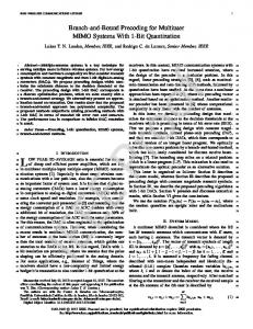
5.1 Adjacency Condition Suppose that jobs i and j are adjacent pairs of jobs before the last position and jobs i and j lie between jobs x and y as shown in figure 1. The total sequencedependent setup cost, TSCij and TSCji, can be calculated using formulas (27) and (28) . TSCij = SCxi + SCij + SCjy
(27)
TSCji = SCxj + SCji + SCiy
(28)
When job i immediately precedes job j, Ωij and Ωji are defined as:
SCij
SCxi x
i
SCiy j
y
Figure 1. Illustration of adjacency condition of jobs i and j.
Ω xy
where
=
⎧0 ⎪ ⎨s x ⎪p ⎩ y
if if if
sx ≤ 0 0 < sx < p y sx ≥ p y
(29)
sx = dx – t – px is the slack of job x. t = the sum of processing times of all preceding jobs.
The following condition must hold for all adjacent pairs of jobs: AJCij = wipj - Ω ij(wi + hi) + TSCji
(30)
AJCji = wjpi - Ω ji(wj + hj) + TSCij
(31)
AJCij ≥ AJCji
(32)
Branch and Bound Approach for Single-Machine Sequencing with …
See the proof of adjacency condition in Appendix A. There are many nodes that are generated from the same parent node. Thus, calculating the adjacency condition using formulas (27) to (32) for all nodes is time consuming. It is possible to reduce the computation time by calculating the adjacency condition only for the first node and using formula (33) for other nodes generated from the same parent node. AJCij + ΔSCjy ≥ AJCji + ΔSCiy
(33)
where ΔSCjy = SCjy of the node under consideration – SCjy of the first node ΔSCiy = SCiy of the node under consideration – SCiy of the first node. Proof: Consider any node generated from the same parent node. Jobs i and j are the same; hence, wipj - Ωij (wi + hi) is equal to wjpi - Ωji (wj + hj). The value of TSCij and TSCji are varied according to the last job. The only differences are SCjy and SCiy. Consequently, the adjacency condition can be computed by adding only the different values (ΔSCjy and ΔSCiy) to the same formula. The adjacency condition can be applied to the node at level 3 and higher. The reason can be shown by the following example. Suppose the node in level 2 is considered, e.g., node (1, 2). Since the setup cost is sequence-dependent, from formulas (27) and (28), SCjy and SCiy, cannot be determined. But if the node is branched further to level 3, e.g., node (1, 2, 3), in this case SCjy is SC23 and SCiy is SC13. 5.2 Non-Adjacency Condition Suppose jobs i and j are non-adjacent pairs of jobs before the last position and they have the same processing time. Job i lies between jobs u and v and job j lies between jobs w and z as shown in figure 2. The total sequence-dependent setup cost, TSCij and TSCji, can be calculated using formulas (34) and (35). t
TSCij = SCui + SCiv + SCwj+ SCjz
(34)
TSCji = SCuj + SCjv + SCwi+ SCiz
(35)
Δij and Δji are defined as: Δ xy
⎧0 ⎪ = ⎨s x ⎪p + K ⎩ y
if if if
sx ≤ 0 0 < sx < p y + K
(36)
sx ≥ p y + K
where sx = dx – t – px is the slack of job x K = the sum of processing times of jobs between jobs i and j All non-adjacent pairs of jobs in the optimal schedule must satisfy the following condition: if pi = pj, then NJCij = wi (pj + K) - Δij (wi + hi) + TSCji
(37)
NJCji = wj (pi + K) - Δji (wj + hj) + TSCij
(38)
NJCij ≥ NJCji
(39)
See the proof of non-adjacency condition in Appendix B. The non-adjacency condition can be applied to the node at level 4 and higher. In other words, at least four jobs must be in the sequence. For example, nonadjacent jobs of the node at level 4 are jobs in positions 1 and 3. The last job in position 4 is used to determine the sequence-dependent setup cost.
6. BRANCH AND BOUND ALGORITHM A network representation and branch and bound algorithm can be used to determine an optimal solution for the problem. A node represents a sub-problem or the sequence of jobs that are already scheduled. An arc leading to the node represents the associated cost of the node. Initialization step
SCui
u
107
SCwj
SCiv
i
v
w
SCjz
j
z
K
Figure 2. Illustration of non-adjacency condition of jobs i and j.
The branch and bound algorithm is started by determining an initial feasible solution to the problem. According to the two-phase heuristic procedures presented in section 4, the priority-dispatching rule is applied to establish the initial sequence. The local improvement procedures are used to modify the schedule obtained in the first phase in order to get a better sequence. The objective function value obtained
108
Chananes Akjiratikarl· Pisal Yenradee
from the two-phase heuristic is an initial upper bound of the objective function value. Steps for each iteration Step 1: Branching The branching strategy is called the depth-first branching rule. Select the active (unfathomed) node at the highest level in the search tree for branching. If there is more than one node at the highest level, select the one with the lowest associated cost. The selected node is called the parent node. Create branches from the parent node to the nodes representing jobs that have not been scheduled. Step 2: Bounding For each newly created node, the associated cost is calculated. The associated cost is the sum of the associated cost of its parent node and the cost due to the newly assigned job of that node. Step 3: Fathoming For each generated node, three computational tests are performed in the fathoming step. First, a node is fathomed if its associated cost is greater than or equal to the current upper bound of the problem (denoted by F1). Second, the dominance criteria described in section 5 are applied to further reduce the number of nodes (denoted by F2). Dominance criteria consist of adjacency and non-adjacency conditions. All pairs of jobs in the optimal schedule must satisfy these conditions. Note that the adjacency condition can be applied to the nodes at level 3 and higher, while the non-adjacency condition can be applied to the nodes at level 4 and higher. If the node is not eliminated by the above two tests, the lower bounds of each of three subproblems are computed according to the procedures presented in section 3. For fast elimination of nodes, the lower bounds of three sub-problems can be calculated in any sequence according to the characteristics of the problem under consideration. Suppose that the sequence of lower bound is LB1, LB2, and MSC. When the LB1 is determined, it is summed to the associated cost of the node and compared with the upper bound. If it is greater than or equal to the current upper bound, the node is fathomed (denoted by F3). If the node is still not fathomed, the LB2 will be computed. The value of LB2 + LB1 + associated cost of the node will be again compared to the upper bound. If the node is still unfathomed, the MSC will be determined. Finally, the sum of lower bounds of three sub-problems (MSC + LB2 +LB1) plus the associated cost of that node is compared to the upper bound. The remaining unfathomed nodes are called active nodes. When a complete sequence is found (all jobs are
scheduled on the node), the node is fathomed (denoted by F4), and its objective function value will be compared with the current upper bound. If the current upper bound is higher, replace the current upper bound by the objective function value of the complete sequence. Optimality test If some active nodes are still available, repeat the iteration steps; otherwise, stop. After the algorithm is terminated, the node in which its objective function value is equal to the current upper bound represents the optimal solution and its objective function value is the optimal total costs.
7. ILLUSTRATIVE EXAMPLE The branch and bound algorithm can be illustrated using the following example. There are 4 jobs to be processed on a single machine. The data of sequencedependent setup cost, processing time, due date, and earliness and tardiness penalties are shown in Table 2 and 3. Table 2. Setup cost matrix. 1
2
3
4
1
0
15
33
3
2
20
0
18
28
3
35
8
0
10
4
2
14
5
0
Table 3. Job information. Job
pi
di
hi
wi
1
3
8
2
9
2
2
6
7
7
3
4
10
3
8
4
3
9
8
6
The priority-dispatching rule generates the sequence of {1, 2, 4, 3} with the total cost of 89. The local improvement procedure modifies the sequence to be {2, 1, 4, 3} with a better total cost of 86, which is
109
Branch and Bound Approach for Single-Machine Sequencing with …
the associated cost and compared to the upper bound. If it is greater than or equal to upper bound, the node is fathomed. In this case, node {4} is fathomed. Then, select job 1 as the branching node because job 1 has the lowest objective function value among the three nodes. Job 1 is now assigned to the first order of the sequence. Then, branch from job 1 for jobs 2, 3, and 4, and place each of jobs 2, 3, and 4 in the second order of the sequence. The associated cost and lower bounds of each node are calculated. Node {1,3} has the associated cost plus lower bounds (LB1+LB2) greater than the upper bound. Thus it is fathomed (making it an inactive node).
used as an initial upper bound for the problem. Figure 3 shows a complete network representation of the illustrative example. In iteration 1, nodes 1, 2, 3, and 4 are constructed, indicating that each of the four jobs could be processed in the first order of the sequence. The associated cost of each node is calculated and shown on an arc leading to that node. Then, the associated cost is compared to the upper bound. The node will be fathomed if the associated cost is higher than or equal to the upper bound. In order to further eliminate these nodes, the lower bounds of the three sub-problems are computed. Each time the lower bound is obtained, it is summed up with
PDR {1,2,4,3} cost = 89 LIP {2,1,4,3} cost = 86 Upper bound = 86 New upper bound = 81 0 54
10 28
1
LB1=0 LB2=6 MSC=16
18
LB1=3 LB2=0 MSC=10
2
LB1=0 LB2=27 MSC=13
3
4
LB1=0 Level 1 LB2=30 MSC=15
F3 3
1 2
LB1=0 LB2=10 MSC=15
5
1 3
3
LB1=0 LB2=39
1 4
5
LB1=0 LB2=30 MSC=13
2 1
1 2 3
68
1 2 4
2 3
LB1=0 LB2=10 MSC=8
F3 53
5
F3 65
1 4 2
42
65
1 4 3
8
LB1=0 LB2=27
2 4
3 1
F1
F3
90
2 1 4
AJCij≥AJCji AJCij