Branch and Bound Methods for. Euclidean Registration Problems. Carl Olsson, Member, IEEE, Fredrik Kahl, Member, IEEE, and Magnus Oskarsson, Member, ...
This article has been accepted for publication in a future issue of this journal, but has not been fully edited. Content may change prior to final publication. IEEE TRANSACTIONS ON PATTERN ANALYSIS AND MACHINE INTELLIGENCE 1
Branch and Bound Methods for Euclidean Registration Problems Carl Olsson, Member, IEEE, Fredrik Kahl, Member, IEEE, and Magnus Oskarsson, Member, IEEE
Abstract— In this paper we propose a practical and efficient method for finding the globally optimal solution to the problem of determining the pose of an object. We present a framework that allows us to use both point-to-point, point-to-line and point-to-plane correspondences for solving various types of pose and registration problems involving Euclidean (or similarity) transformations. Traditional methods such as the iterative closest point algorithm, or bundle adjustment methods for camera pose, may get trapped in local minima due to the non-convexity of the corresponding optimization problem. Our approach of solving the mathematical optimization problems guarantees global optimality. The optimization scheme is based on ideas from global optimization theory, in particular, convex under-estimators in combination with branch and bound methods. We provide a provably optimal algorithm and demonstrate good performance on both synthetic and real data. We also give examples of where traditional methods fail due to the local minima problem. Index Terms— Registration, camera pose, global optimization, branch and bound.
I. I NTRODUCTION FREQUENTLY occurring, and by now a classical problem in computer vision, robotic manipulation and photogrammetry is the registration problem, that is, finding the transformation between two coordinate systems, see [1, 2, 3]. The problem appears in several contexts: relating two stereo reconstructions, solving the hand-eye calibration problem and finding the absolute pose of an object, given 3D measurements. A related problem is the camera pose problem, that is, finding the perspective mapping between an object and its image. In this papper, we will develop algorithms for computing globally optimal solutions to these registration problems within the same framework. There are a number of proposed solutions to the registration problem and perhaps the most well-known is by Horn et al. [4]. They derive a closed-form solution for the Euclidean (or similarity) transformation that minimizes the sum of squares error between the transformed points and the measured points. As pointed out in [5], this is not an unbiased estimator if there are measurement errors on both point sets. The more general problem of finding the registration between two 3D shapes was considered in [6], where the iterative closest point (ICP) algorithm was proposed to solve the problem. The algorithm is able to cope with different geometric primitives, such as point sets, line segments and different kinds of surface representations. However, the algorithm requires a good initial transformation in order to converge to the globally optimal solution, otherwise only a local optimum is attained. A number of approaches have been devoted to make the algorithm more robust to such difficulties, e.g. [7, 8], but the algorithm is still plagued by local minima problems. In [9], a (local) convergence analysis for algorithms similar to ICP is given. Further more a comparison with respect to global convergence is given.
A
Digital Object Indentifier 10.1109/TPAMI.2008.131
In this paper, we generalize the method of Horn et al. [4] by incorporating point, line and plane features in a common framework. Given point-to-point, point-to-line, or point-to-plane correspondences, we demonstrate how the transformation (Euclidean or similarity) relating the two coordinate systems can be computed based on a geometrically meaningful cost function. However, the resulting optimization problem becomes much harder - the cost function is a polynomial function of degree four in the unknowns and there may be several local minima. Still, we present an efficient algorithm that guarantees global optimality. A variant of the ICP-algorithm with a point-to-plane metric was presented in [8] based on the same idea, but it is based on a local, iterative optimization method. The camera pose problem has been studied for a long time, that is estimating the camera pose given 3D points and corresponding image points. The minimal amount of data required to solve this problem is three point correspondences and for this case there may be up to four solutions. The result has been shown a number of times, but the earliest solution is to our knowledge due to Grunert, already in 1841, [10]. A good overview of the minimal solvers and their numerical stability can be found in [11]. Given at least six point correspondences the predominant method to solve the pose estimation problem is by estimating the solution linearly using the DLT algorithm, and then use this as a starting solution for a gradient descent method, see [2, 12, 3]. There are also quasi-linear methods that give a unique solution given at least four point correspondences, see [13, 14]. These methods solve a number of algebraic equations, and do not minimize the reprojection error. Given a Gaussian noise model for the image measurements and assuming i.i.d. noise, the Maximum Likelihood (ML) estimate is computed by minimizing the norm of the reprojection errors. To our knowledge, there are no previous algorithms that have any guarantee of obtaining the globally optimal ML solution. The algorithms presented in this paper are based on relaxing the original non-convex problems by convex under-estimators and then using branch and bound to focus in on the global solution [15]. The under-estimators are obtained by replacing bilinear terms in the cost function with convex and concave envelopes, see [16] for further details. Branch and bound methods have been used previously in the computer vision literature. For example, in [17] various multiple view geometry problems are considered in a fractional programming framework. In summary, our main contributions are: • A generalization of Horn’s method for the registration problem using points, lines and planes. • An algorithm for computing the global optimum of the corresponding quartic polynomial cost function. • An algorithm for computing the global optimum to the camera pose problem. • The introduction of convex and concave relaxations of
0162-8828/$25.00 © 2008 IEEE
This article has been accepted for publication in a future issue of this journal, but has not been fully edited. Content may change prior to final publication. IEEE TRANSACTIONS ON PATTERN ANALYSIS AND MACHINE INTELLIGENCE 2
where T is in the set of feasible transformations. In the case of a similarity transform T (x) = sRx + t, with s ∈ R+ , R ∈ SO(3) and t ∈ R3 . (s = 1 corresponds to the Euclidean case). Our goal is to find the global optimum of problem (2). Note that the sets Ci do not have to be distinct. If two points xi and xj map to the same set then we take Ci = Cj . The following theorem shows why it is convenient to only work with convex sets. Theorem 1: dC is a convex function if and only if C is a convex set. Proof: Since C can be written as the zero level set { x ; dC (x) ≤ 0 }, C must be convex if dC is convex. Next assume that C is convex. Let z = λx + (1 − λ)y for some scalar λ ∈ [ 0 , 1 ]. Pick x� , y � , z � ∈ ∂C such that dC (x) = min ||x − u|| = ||x − x� ||
(3)
dC (y) = min ||y − u|| = ||y − y � ||
(4)
u∈C
u∈C
�
dC (z) = min ||z − u|| = ||z − z || u∈C
(5)
Since d is a norm and λx� + (1 − λ)y � ∈ C we obtain dC (λx + (1 − λ)y)
Fig. 1.
The experimental setup for the tests done in Section V-C.
monomials in the computer vision literature. This opens up the possibility of attacking similar problems for which so far only local algorithms exist. Although we only give experimental results for point, line and plane correspondences, it is shown that our approach is applicable to more general settings. In fact, correspondence features involving any convex sets can be handled. The work in this paper is based on the conference papers [18, 19]. II. A G ENERAL P ROBLEM F ORMULATION We will now make a general formulation of the problem types we are interested in solving. The stated problem is to find a transformation relating two coordinate systems; the model coordinate system and the measurement coordinate system. In the measurement system we have points that we know should map to some convex sets in the model system. Typically, in a practical situation, the convex sets consist of single points, lines or planes, but in principle, they may be any convex set. We want to determine a transformation such that the mapping of the measurement points come as close to their corresponding convex sets as possible. The transformation is usually a similarity or a Euclidean transformation. We will also consider the transformation consisting of a Euclidean transformation followed by a perspective mapping in the camera pose problem. Let || · || be any norm. We define the distance from a (closed) set C as dC (x) = min ||x − y||. (1) y∈C
{xi }m i=1
{Ci }m i=1
be the point measurements and be the Let corresponding model sets. The registration (or pose) problem can then be written as min T
m X i=1
dCi (T (xi )),
(2)
=
||z − z � || ≤ ||z − (λx� + (1 − λ)y � )||
≤
λ||x − x� || + (1 − λ)||y − y � ||
=
λdC (x) + (1 − λ)dC (y).
(6)
The inequality ||z − z � || ≤ ||z − (λx� + (1 − λ)y � )|| is true since z � = argminu∈C ||z − u||. Theorem 1 shows that if T depends affinely on some parameters then problem (2) is a convex optimization problem in these parameters, which can be solved efficiently using standard optimization methods [20]. This is however not the case for Euclidean and similarity transformations. In these cases (2) becomes highly non convex due to the orthogonality constraints RT R = I . Instead we will use larger sets of transformations, that can be parameterized as affine combinations of some parameters, and use (2) to obtain lower bounds. These bounds can then be used to find the global optimum in a branch and bound scheme. Note that the convexity of dC does not depend on the particular choice of norm. We will typically use the 2-norm ||x||2 = xT x but our methods are easily extended to norms such as ||x||A = xT Ax where A is a positive definite matrix, making it possible to include uncertainty weights. III. G LOBAL O PTIMIZATION In this section we briefly present some notation and concepts of convex optimization and branch and bound algorithms. This is standard material in (global) optimization theory. For a more detailed introduction see [20] and [15]. A. Convex Optimization A convex optimization problem is a problem of the form min
such that
g(x) hi (x) ≤ 0,
i = 1, ..., m.
(7)
Here x ∈ Rn and both the cost (or objective) function g(x) : Rn �→ R and the constraint functions hi (x) : Rn �→ R are convex functions. Convex problems have the very useful property that a local minimizer to the problem is also a global minimizer. Therefore it fits naturally into our framework.
This article has been accepted for publication in a future issue of this journal, but has not been fully edited. Content may change prior to final publication. IEEE TRANSACTIONS ON PATTERN ANALYSIS AND MACHINE INTELLIGENCE 3
The convex envelope of a function h : S �→ R (denoted hconv ) is a convex function which fulfills: 1) hconv (x) ≤ h(x), ∀x ∈ S . 2) If u(x) is convex on S and u(x) ≤ h(x), ∀x ∈ S then hconv (x) ≥ u(x), ∀x ∈ S . Here S is a convex domain. The concave envelope is defined analogously. The convex envelope of a function has the nice property that it has the same global minimum as the original function. However computing the convex envelope usually turns out to be just as difficult as solving the original minimization problem. B. Branch and Bound Algorithms Branch and bound algorithms are iterative methods for finding global optima of non-convex problems. They work by calculating sequences of provable lower bounds which converge to the global minimum. The result of such an algorithm is an �−suboptimal solution, that is, a solution that gives a cost of at most � more than the global minimum. By setting � small enough, we can get arbitrarily close to the global optimum. The idea of branch and bound is simple and straightforward, and at the same time very powerful. Suppose that computing the global minimum directly of the objective function f (t) over a set D0 is too hard. Instead we first construct a lower bounding function flower (t) over the domain D0 and then minimize flower (t) over D0 . Hence, we require that flower (t) ≤ f (t) for all t ∈ D0 and that computing the minimum of flower is (relatively) easy. If the difference between the bounding function and the original cost function when evaluated at the minimum of flower is less than �, then we have found our �−suboptimal solution. Otherwise, we subdivide (branch) the set D0 into smaller sets and perform bounding on each subset. If the lower bound for a subset is higher than the value of the best solution found so far, then this subset can be discarded from further consideration. Again, if the difference between the lower bounding function and the cost function (at the optimum of the lower bounding function) is larger than � we need to subdivide the set further. This process is repeated until the global minimum has been found. In order for this procedure to converge, there are some requirements that the bounding function must fulfill. Let us examine these conditions more closely. Consider the following (abstract) problem. We want to minimize a non-convex scalar-valued function f (t) over a set D0 . One may assume that D0 is closed and compact so a minimum is attained within the domain. For any closed set D ⊂ D0 , let fmin (D) denote the minimum value of f on D and let flower (D) denote the minimum value of the lower bounding function flower (t) on D, that is, flower (D) = mint∈D flower (t). Also we require that the approximation gap fmin (D)−flower (D) goes uniformly to zero as maxx,y∈D ||x − y|| (denoted |D|) goes to zero. Or in terms of (�, δ), we require that ∀� > 0, ∃δ > 0 s.t. ∀D ⊂ D0 , |D| ≤ δ ⇒ fmin (D) − flower (D) ≤ �.
If such a lower-bounding function flower can be constructed then a strategy to obtain an �-suboptimal solution is to divide the domain into sets Di with sizes |Di | ≤ δ and compute flower (Di ) in each set. However the number of such sets increases quickly with 1/δ and therefore this may not be feasible. To avoid this
problem a strategy to create as few sets as possible can be deployed. Assume that we know that fmin (D0 ) < l for some scalar l. If flower (D) > l for some set D then there is no point in refining D further since the global minimum will not be contained in D. Thus D and all possible refinements Di ⊆ D can be discarded. The branch and bound algorithm begins by computing flower (D0 ) and the actual point t∗ ∈ D0 which is the minimizer. This is our current best estimate of the minimum. If f (t∗ ) − flower (D0 ) ≤ � then t∗ is �-suboptimal and the algorithm terminates. Otherwise the set D0 is partitioned into subsets (D1 , ..., Dk ) with k ≥ 2 and one gets the lower bounds flower (Di ) and the points t∗i in which these bounds are attained. The new best estimate of the minimum is t∗ := argmin{t∗ }k f (t∗i ). If f (t∗ ) − min1≤i≤k flower (Di ) ≤ �, then t∗ i i=1 is �-suboptimal and the algorithm terminates. Otherwise the subsets are refined further, however, the sets for which flower (Di ) > f (t∗ ) can be discarded immediately and need not be considered for further computations. This algorithm is guaranteed to find an �-suboptimal solution for any � > 0. The drawback is that the worst case complexity is exponential. In practice one can achieve relatively fast convergence if the obtained bounds are tight. In most cases we do not want to minimize the function over the entire domain, but rather to a subset. Then we also need to check if the problem is feasible in each set Di - if it is not, the set can be removed from further consideration. IV. C ONVEX R ELAXATIONS OF SO(3) In this section we derive relaxations of SO(3) and the group of similarity transformations that allows us to parametrize the transformations affinely. The goal is to obtain easily computable lower bounding functions for cost functions involving Euclidean transformations. Recall from Section II that problem (2) is convex if T depends affinely on its parameters. A common way to parametrize rotations is to use quaternions (see [21]). Let q = (q1 , q2 , q3 , q4 )T , with ||q|| = 1 be the unit quaternion parameters of the rotation matrix R. If the scale factor s is free to vary, one can equivalently drop the condition ||q|| = 1. We note that for a point x in R3 , we can rewrite the 3-vector sRx as a vector containing quadratic forms in the quaternion parameters in the following way 1 q T B1 (x)q C B sRx = @ q T B2 (x)q A T q B3 (x)q 0
(8)
where Bl (x), l = 1, 2, 3 are 4 × 4 matrices whose entries depend on the elements of the vector x. In order to be able to use the branch and bound algorithm, it is required that we have bounds on q such that qiL ≤ qi ≤ qiU , i = 1, 2, 3, 4. In practice these bounds are usually known since the scale factor cannot be arbitrarily large. The quadratic forms q T Bl (x)q contain terms of the form blij (x)qi qj , and therefore we introduce new variables sij = qi qj , i = 1, .., 4, j = 1, ..., 4 in order to linearize the problem. Now consider the constraints sij = qi qj , or equivalently sij ≤ qi qj ,
(9)
sij ≥ qi qj .
(10)
This article has been accepted for publication in a future issue of this journal, but has not been fully edited. Content may change prior to final publication. IEEE TRANSACTIONS ON PATTERN ANALYSIS AND MACHINE INTELLIGENCE 4
In the new variables sij , the cost function becomes convex, cf. (2), but the domain of optimization given by the above constraint functions is not a convex set. The constraints (10) are convex if i = j and (9) is not convex for any i, j . If we replace qi qj in (9) with the concave envelope of qi qj then (9) will be a convex condition. We also see that by doing this we expand the domain for sij and thus the minimum for this problem will be lower or equal to the original problem. Similarly we can relax qi qj in (10) by its convex envelope and obtain a convex problem which gives a lower bound on the global minimum of the cost function (2). The convex envelope of qi qj , i = j , qiL ≤ qi ≤ qiU , qjL ≤ qj ≤ U qj , is well known (e.g., [16]) to be (
(qi qj )conv = max
qi qjU + qiU qj − qiU qjU qi qjL + qiL qj − qiL qjL
and the concave envelope is (
(qi qj )conc = min
qi qjL + qiU qj − qiU qjL qi qjU + qiL qj − qiL qjU
)
≤ qi qj ,
(11)
≥ qi qj .
(12)
)
Thus the equations (9) and (10) for i = j can be relaxed by the linear constraints −sij + qi qjU + qiU qj − qiU qjU ≥ 0,
(13)
−sij + qi qjL + qiL qj − qiL qjL ≥ 0, sij − (qi qjL + qiU qj − qiU qjL ) ≥ 0, sij − (qi qjU + qiL qj − qiL qjU ) ≥ 0.
(14) (15)
1
0.8
0.8
0.6
0.6
0.4
0.4
0.2
0.2
0
0
−0.2 −1
0 q1
1
−0.2 −1
subject to
ˆ
q + t) i=1 dC (B(xi )ˆ sjj − qj2 ≥ 0, T
j = 1, . . . , 4,
c − A qˆ ≥ 0, S 0.
(17)
In the case of finding a Euclidean transformation instead of a similarity transformation we can simply add the extra linear constraint s11 + s22 + s33 + s44 − 1 = 0.
(18)
Thus, the original non-convex problem has been convexified by expanding the domain of optimization, and hence the optimal solution to the relaxed problem will give a lower bound on the global minimum of the original problem. Implementation
s11
1
s11
1.2
Pm
minqˆ,t
(16)
If i = j we need to relax qi2 in (9) with its concave envelope. However this is simply a line aqi +b, where a and b are determined by noting that the values (qiL )2 and (qiU )2 should be attained at the points qi = qiL and qi = qiU , respectively. Figure 2 shows the upper and lower bounds of s11 when −1 ≤ q1 ≤ 1. We see that even when the interval has only been divided four times the upper bound is quite close to the lower bound. This gives some indication on how the lower bounds on the problem may converge quite rapidly. Since all the non-convex constraints 1.2
domain these lower bounds will tend to the global minimum of the original problem. To summarize we now state the relaxed problem which will serve as a bounding function in our branch and bound algorithm. For now we restrict T to be the set of Euclidean (or similarity) transformations, that is, x �→ Rx + t where R denotes a rotation matrix and t a translation vector. In a later section we will generalize this to include perspective mappings in order to solve the camera pose problem. Let qˆ be a 14 × 1 vector containing the parameters (q1 , ..., q4 , s11 , s12 , ..., s44 ). The quadratic forms q T Bl (xi )q in (8) can then be relaxed by the terms bl (xi )T qˆ where bl (xi ) is a vector of the same size as qˆ whose entries depend on xi . Note that entries of bl (xi ) are obtained directly from the ˆ i )ˆ entries of Bl (xi ). The vector sRxi can now be written B(x q T ˆ where B(xi ) is a 3 × 14 matrix with rows bl (xi ) . All the linear constraints in (13)-(16) as well as the bounds on the quaternion parameters qi can be written as cj − aTj qˆ ≥ 0 where cj is a constant and aj is a vector of same size as qˆ. These constraints can be written as a matrix inequality c − AT qˆ ≥ 0 where c is a vector whose entries are the cj and A is a matrix whose columns are the aj ’s. To improve the bound further we may also add the constraint that the symmetric matrix S with entries sij in position (i, j) should be positive definite. (note that sij = sji .) Then the relaxed problem can be written, cf. (2),
0 q1
1
Fig. 2. Upper and lower bounds of s11 , which relaxes q12 in the interval [ −1 , 1 ]. Left: the initial bound. Right: when the interval has been subdivided four times. Note that the lower bound is exact since q12 ≤ s11 is convex.
have been replaced by convex constraints, the relaxed problem is now convex. Thus we can minimize this problem to obtain a lower bound on the original problem and as we subdivide the
The implementation of the algorithm was done in Matlab. We basically used the algorithm described in Section III-B and the relaxations from Section IV. At each iteration, problem (17) is solved for all rectangles Di to obtain a lower bound on the function over Di . To speed up convergence we use the minimizer t∗i of the problem (17) as a starting guess for a local minimization of the original non-convex problem. We then compare the function value at the local optimizer tloc and at t∗i . If any of these values i are lower than the current best minimum the lowest one is deemed the new best minimum. Even though t∗i is the optimal value of the relaxed problem (17) it is often the case that the function values are larger at t∗i than at tloc i . Therefore we reach lower values faster if we use the local optimizer and thus intervals can be thrown away faster. If an interval is not thrown away then we subdivide it into two. We divide the intervals along the dimension which has the longest side. In this way the worst case would be that the number of intervals doubles at each iteration. However we shall see later that in practice this is not the case. As a termination criterion we use the total 4-dimensional volume of the rectangles. One could argue that it would be sufficient to terminate when the
This article has been accepted for publication in a future issue of this journal, but has not been fully edited. Content may change prior to final publication. IEEE TRANSACTIONS ON PATTERN ANALYSIS AND MACHINE INTELLIGENCE 5
approximation gap (see Section III-B) is small enough, however this does not necessarily mean that the �-suboptimal solution is close to the real minimizer. To solve the relaxed problem we used SeDuMi (see [22]). SeDuMi is a free add-on for Matlab that can be used to solve problems with linear, quadratic and semi-definiteness constraints. For the local minimization we used the built in Matlab function fmincon. V. A PPLICATIONS I: R EGISTRATION U SING P OINTS , L INES AND / OR P LANES We will now review the methods of Horn et al. as presented in [4]. Given two corresponding point sets we want to find the best transformation that maps one set onto the other. The best is here taken to mean the transformation that minimizes the sum of squared distances between the points, i.e. m X
||T (xpi ) − ypi ||22 ,
Corresp. type Point-Point Point-Plane Point-Line Combination
with s ∈ R+ , R ∈ SO(3) and t ∈ R3 (s = 1 corresponds to the Euclidean case). Following Horn [4], it is easily shown that the optimal translation t is given by t=
1 X 1 X xp . ypi − R xpi = y¯p − R¯ m m
(20)
This will turn equation (19) for the Euclidean case into m X
||Rδxi − δyi ||22 =
(21)
i=1
=
m X
(δxi )T δxi + (δyi )T δyi − 2(δyi )T Rδxi ,
(22)
i=1
with δxi = xpi − x ¯p and δyi = ypi − y¯p . Due to the orthogonality of R this expression becomes linear in R. Now R can be determined from the singular value decomposition of a matrix constructed from δxi and δyi . The details can be found in [4]. In this application we will consider not only point-to-point correspondences but also point-to-line and point-to-plane correspondences. In the following sections it will be shown why the extension to these types of correspondences result in more difficult optimization problems. In Figure 1, a measurement device is shown which generates 3D point coordinates and which will be used for validation purposes. Table I describes different methods available for global optimization. Note that if the transformation considered is affine, i.e. T (x) = Ax + t, then the problem is simply a linear least squares problem. A. Point-to-Plane Correspondences We will now consider the point-to-plane problem. Suppose we have a number of planes πi in one coordinate system and points xπi i = 1, ..., mπ in another, and we assume that point yπi lies on plane πi . Let dπ (x) be the minimum distance between a point
Linear Linear Linear Linear
Least Least Least Least
Squares Squares Squares Squares
DIFFERENT TYPES OF CORRESPONDENCES AND TRANSFORMATIONS .
x and a plane π . The problem is now to find s ∈ R+ , R ∈ SO(3) and t ∈ R3 that minimizes fπ (s, R, t) =
mπ X
(dπi (sRxπi + t))2 .
(23)
i=1
From elementary linear algebra we know that this can be written as
(19)
T (x) = sRx + t,
Affine
TABLE I M ETHODS AVAILABLE FOR ESTIMATING THE REGISTRATION FOR
fπ (s, R, t) =
i=1
where xpi and ypi , i = 1, .., m, are the 3D points in the respective coordinate systems. Here we assume T to be either a Euclidean or a similarity transformation,
Euclidean/ Similarity Horn [4] Our algorithm Our algorithm Our algorithm
mπ X
((sRxπi + t − yπi ) · ni )2 ,
(24)
i=1
where ni is a unit normal of the plane πi and · is the inner product in R3 . Thus we want to solve the problem s∈R+
mπ “ X
min
,R∈SO(3),t∈R3
nT i (sRxπi + t − yπi )
”2
.
(25)
i=1
In order to reduce the dimensionality of this problem we now derive an expression for the translation t. This is similar to the approach by Horn et. al. (see [4]) in which all measurements are referred to the centroids. If we let R be any 3×3 matrix we can consider the problem (25) as minimizing (24) with the constraints gij (s, R, t) = riT rj − δij i, j = 1, 2, 3, where ri is the columns of R and δij is the Dirac function. From the method of Lagrange multipliers we know that for a local minimum (s∗ , R∗ , t∗ ) (and hence a global) there must be numbers λi,j such that ∇fπ (s∗ , R∗ , t∗ ) +
3 3 X X
λij ∇gij (s∗ , R∗ , t∗ ) = 0.
(26)
i=1 j=1
Here the gradient is taken with respect to all parameters. We see that the constraint is independent of the translation t, thus it will disappear if we apply the gradient with respect to t. Moreover we see that we will get a linear expression in t and, thus we are able to solve for t. It follows that t = N −1 P
mπ X
ni nT i (yπi − sRxπi ),
(27)
i=1
T π where N = m j=1 nj nj . Note that if N is not invertible then there are several solutions for t. However if t and t˜ are two such solutions then their P ˆ difference tˆ = t − t˜ is in the null space of N thus nj nT j t = 0. Now one can easily prove by inserting t˜ into the cost function (24) that fπ (s, R, t˜) = fπ (s, R, t). This means that there in this case are infinitely many solutions and thus the problem is not well-posed. Next we state the relaxed problem in the form similar to (17). In this case the distance function is dπi (x) = (nTi (x − yπi ))2 . If we parametrize the problem using quaternions as in (17) and
This article has been accepted for publication in a future issue of this journal, but has not been fully edited. Content may change prior to final publication. IEEE TRANSACTIONS ON PATTERN ANALYSIS AND MACHINE INTELLIGENCE 6
local min point (0, -0.078, -1.00, -0.49) (0, 0.12, -0.33, -0.93) (0.59, 0.042, 0.70, 0.41) (0.66, 0.22, 0.72, 0.23) (0,0,0,0)
introduce the relaxations in terms of the qˆ paramameters we get mπ X i=1
dπi (sRxπi + t) =
mπ X
ˆ ˆ − yπi ))2 = (nT i (Bi q
i=1
mπ X
˜i qˆ − ki )2 (B
i=1
(28) ˜i = nT B ˆi is a 1 × 14 vector and ki = nT yπi . Together where B i i with the constraints from (17) this gives us our relaxed lower bounding problem. Note that it is easy to incorporate uncertainty ˜i and ki by wi B ˜i and weights into (28) simply by replacing B wi ki respectively. B. Point-to-Line and Point-to-Point Correspondences The case of point-to-line correspondences can be treated in a similar way as in the case of point-to-plane correspondences. Let xli , i = 1, ..., ml , be the measured 3D points and let li , i = 1, ..., ml , be the corresponding lines. In this case the sum of the distance functions can be written as dli (x) = ||(I − vi viT )(x − yli )||2
(29)
where vi is a unit direction vector for the line li and yli is any point on the line li . Note that the three components of (I − vi viT )(x − yli ) are linearly dependent since (I − vi viT ) is a rank 2 matrix. However it would not make sense to remove any of them since we would then not be optimizing the geometrical distance any more. In the same way as in the point-to-plane we can eliminate the t parameters and write our cost function in the form (28). The case of point-to-point correspondences is the easiest one. Let xpi be the measured points and ypi be the corresponding points i = 1, ..., mp . the distance function is just dypi (x) = ||x − ypi ||2 .
(30)
cost function value 2.1 2.2 0.00037 0.0018 65
TABLE II L OCAL MINIMA FOUND BY THE M ATLAB FUNCTION fmincon.
function-values along a line from one local minimum to the global minimum. To the left is the values on the line from the first point in Table II and on the right is the second point. 100
100
90
90
80
80
70
70
60
60
50
50
40
40
30
30
20
20
10
10
0
0
0.5
1
0
0
0.5
1
Fig. 3. The function values on two lines between a local minimum and the global minimum.
Iterations: Figure 4 shows the performance of the algorithm in two cases. In both cases the data has been synthetically generated. The first problem is the case of ten point-to-plane, four point-toline and four point-to-point correspondences. The solid line to the left in Figure 4 shows the number of feasible rectangles for this problem at each iteration. For each rectangle the algorithm solves the program (17) using the standard solver SeDuMi [22] with Matlab. The solid line to the right shows the fourth root of the „X mp ml X −1 T total volume of the rectangles. Recall that this is a 4-dimensional t =M (ypi − Rxpi ) + (I − vi vi )(yli − Rxli ) + problem and therefore the fourth root gives an estimate of the i=1 i=1 « total length of the sides in the rectangles. This case exhibits the mπ X + ni nT (31) typical behavior for this algorithm. The total execution time for i (yπi − Rxπi ) i=1 this problem is around 10 seconds. The second case is the minimal Pml Pmπ T T where M = mp I + i=1 (I −vi vi )+ j=1 nj nj . Substituting case of 7 point-to-plane correspondences. This seems to be the this into the cost function we can now find an expression of the case where our algorithm has the most difficulties. The dashed lines shows the performance for this case. Note that this case type (28). could probably be solved much more efficiently with a minimal case solver, it is merely included to show the worst case behavior C. Experiments and Results of the algorithm. The total execution time for this problem is Local Minima: Non-convex problems usually exhibit local around 30 seconds. For comparison the dotted line to the left minima. To show some typical behavior of these kinds of shows what the number of rectangles would be if no rectangles functions we generated a problem with 8 plane-to-point corre- where thrown away. In the first case the algorithm terminated spondences. This was done in the following way. We randomly after 38 iterations, and in the second after 39, which is a typical generated 8 planes πi and then picked a point yπi from each behavior of the algorithm. Experiments on Real Data: Next we present two experiments plane. Then the points xπi = RT (yπi − t) were calculated for known R and t. We used the Matlab built-in function fmincon to made with real data. The experimental setup can be viewed in search for the minima from some different starting points. Table II figure 1. We used a MicroScribe-3DLX 3d scanner to measure the shows the results. Note that the third point is the global minimum. 3D-coordinates of some points on two different objects. The 3DTo get an idea of the shape of the function, Figure 3 plots the scanner consists of a pointing arm with five degrees of freedom
Again our cost function can be put in the same form as (28). When we have combinations of different correspondences we proceed in exactly the same way. Note however that we have to add the cost functions before eliminating the t-variables since they will depend on all the correspondences. When doing this one gets the expression for t as
This article has been accepted for publication in a future issue of this journal, but has not been fully edited. Content may change prior to final publication. IEEE TRANSACTIONS ON PATTERN ANALYSIS AND MACHINE INTELLIGENCE 7
35
1.8
residuals are the squared distances. The first nine are the pointto-plane, the next two are the point-to-line and the last four are the point-to-point correspondences. We see that the point-to-point
1.6
30
1.4 25
1.2
20
1
15
0.8
−3
1.8
−3
x 10
1.8
1.6
1.6
1.4
1.4
1.2
1.2
1
1
0.8
0.8
0.6
0.6
0.4
0.4
0.2
0.2
x 10
0.6
10
0.4 5
0.2
0 0
20
0 0
40
20
40
Fig. 4. Left, the number of feasible rectangles at each iteration for two experiments (solid and dashed lines, see text for details). For compairison the dotted line shows the theoretical worst case preformance where no intervalls are discarded. Right, the fourth root of the total volume of the rectangles.
and a foot pedal. It can be connected to the serial-port on a PC. To measure a 3D-coordinate one simply moves the pointing arm to the point and presses the pedal. The accuracy of the device is not very high. If one tries to measure the same point but varies the pose of the pointer one can obtain results that differ by approximately half a millimeter. The test objects are the ones that are visible in figure 1, namely the Rubik’s cube and the toy model. By request of the designer will refer to the toy model as the space station. a) Rubik’s Cube Experiment.: The first experiment was done by measuring on a Rubik’s cube. The Rubik’s cube contains both lines planes and points and therefore suits our purposes. We modeled three of the sides of the cube and we measured nine point-to-plane, two point-to-line and three-point-to-point correspondences on these sides. Figure 5 shows the model of the Rubik’s cube and the points obtained when applying the estimated transformation to the measured data points. The points marked
3 2 1 0
3 3
2
2
5
10
15
0 0
5
10
0
0
The model of the Rubik’s cube.
with crosses are points measured on the planes, the points marked with rings are measured on lines and the points marked with stars are measured on corners. It is difficult to see from this picture how well the points fit the model, however to the left in figure 6 we have plotted the residual errors of all the points. Recall that the
15
Fig. 6. Left, Residual errors for all correspondences. Right, Leave-one-out residuals. (see text for details)
residuals are somewhat larger than the rest of the residuals. There may be several reasons for this, one is that using the 3D-scanner it is much harder to measure corners than to measure planes or lines. This is because a corner is relatively sharp and thus the surface to apply the pointer to is quite small making it easy to slip. To the right in figure 6 is the result from a leave-one-out test. Each bar represents an experiment where we leave one data point out, calculate the optimal transformation and measure the residual of the left out point. Again the first nine are the pointto-plane, the next two are the point-to-line and the last four are the point-to-point correspondences. For comparison we also implemented the algorithm by Horn et. at. [4] and an algorithm based on linear least squares. The last algorithm first finds an optimal affine transformation y = Ax + b and then finds sR by minimizing ||A − sR||F where || · ||F is the frobenius norm. The translation is then calculated from equation (31). Note that in order to calculate the affine transformation one needs at least 12 equations. Table III shows the results obtained from the three methods when solving the Rubik’s cube experiment. The residuals stated are the sum of the different types of correspondence residuals. Note that this experiment is somewhat unfair to the algorithm by Horn et. at. since it only optimizes the point-to-point correspondences. However due to the lack of other alternatives we still use it for comparison. As one would expect the solution obtained by Horn’s algorithm has a lower residual sum for the point-to-point correspondences, since this is what it optimizes. Our algorithm has a lower total residual sum since this is what we optimize.
1
1
Fig. 5.
0 0
Residuals: point-point point-line point-plane Total
Our Alg. 0.0023 4.7e-04 0.0018 0.0045
Horn 1.3e-04 0.0016 0.0095 0.0113
Lin. least sq. 0.0051 0.0027 0.0049 0.0127
TABLE III R ESIDUALS OF THE CUBE PROBLEM .
This article has been accepted for publication in a future issue of this journal, but has not been fully edited. Content may change prior to final publication. IEEE TRANSACTIONS ON PATTERN ANALYSIS AND MACHINE INTELLIGENCE 8
Residuals: point-point point-line point-plane Total
Space Station Experiment.: The next experiment was done by measuring on the space station. It is slightly more complicated than the Rubik’s cube and it contains more planes to measure from. We measured 27 point-to-plane, 12 point-to-line and 10point-to-point correspondences on the space station. Figure 7 shows the model of the space station and the points obtained when applying the estimated transformation to the measured data points.
Our Alg. 0.0083 0.0018 0.0046 0.0147
Horn 0.0063 0.0036 0.0098 0.0197
Lin. least sq. 0.0221 0.0015 0.0046 0.0282
TABLE IV R ESIDUALS OF THE SPACE STATION PROBLEM .
1 0.5 0 2
3
1.5
2.5
1
2
0.5
1.5 0 −0.5 0
The model of the Space Station.
To the left in figure 8 we have plotted the residual errors of all the points, and to the right are the results of the leave-one-out test. −3
2
−3
x 10
2
1.8
1.8
1.6
1.6
1.4
1.4
1.2
1.2
1
1
0.8
0.8
0.6
0.6
0.4
0.4
0.2
0.2
0 0
20
40
Chair experiment with 3D-scanner.
0.5 −1
Fig. 7.
Fig. 9.
1
x 10
0 0
The residuals for the point-point correspondences will be lower for Horn’s method as expected while the total error is larger than our algorithm. By approximating the Eucldian transformation by an affine one, the problem becomes a linear least squares problem. An Euclidean transformation can be obtained a posteriori from the affine estimate by taking the closest Euclidean transformation. As can be seen in the table, the linear algorithm does ok, but the optimum is not obtained. Residuals: point-point point-line point-plane Total
Our Alg. 0.0286 6.0630e-04 0.0118 0.0410
Horn 0.0220 0.4986 0.0404 0.5610
Lin.Least Sq. 0.0316 0.0072 0.0111 0.0499
TABLE V R ESIDUALS OF THE SIMULATED DATA FOR THE E UCLIDEAN ALGORITHM .
VI. A PPLICATIONS II: C AMERA P OSE U SING P OINTS 20
40
Fig. 8. Left, Residual errors for all correspondences. Right, Leave-one-out residuals. (see text for details)
Table III shows the results obtained from the three methods when solving the space station experiment. Note that in this case the algorithm by Horn et. at. [4] preforms better since we have included more point-to-point correspondences then in the Rubik’s cube experiment. Again our algorithm has the lowest total residual sum, while Horn has the lowest point-to-point residual. Experiments on Synthetic Data: A Comparison with Horn: For completeness we also include an experiment where the Euclidean version of the algorithm is tested against the Euclidean versions of Horn and the linear least squares. We artificially generated six point-to-point, three point-to-line and seven pointto-plane correspondences. The results can be seen in Table V.
One of the basic problems both in computer vision and in photogrammetry is the camera pose estimation problem. Given a number of correspondences between points in 3D space and the images of these points, the pose estimation problem consists of estimating the rotation and position of the camera. Here the camera is assumed to be calibrated. A typical application is shown in Figure 9, where the object is to relate a camera to a scanned 3D model of a chair. Given m world points Xi (represented by 3-vectors) and ˜T ˆ corresponding image points xi = x1i x2i , we want to find the camera translation t and rotation R that minimizes f :
=
Pm
i=1
P 2 f (R, t) = m i=1 d(xi , π(Xi )) = „ «2 „ «2 ! r1T Xi +t1 r2T Xi +t2 1 2 xi − rT X +t , (32) + xi − rT X +t 3
i
3
3
i
3
T ˆ where π(·) ˜ is Tthe ˆperspective ˜ projection with R r1 r2 r3 and t = t1 t2 t3 .
=
This article has been accepted for publication in a future issue of this journal, but has not been fully edited. Content may change prior to final publication. IEEE TRANSACTIONS ON PATTERN ANALYSIS AND MACHINE INTELLIGENCE 9
Recall that the problem is to find a rotation R and a translation t such that (32) is minimized which is similar to the registration problem in Section V. Using unit quaternions for parametrizing the rotation matrices, the cost function (32) can be rewritten as f (q, t) =
2m X i=1
q T Ai q + aT i t q T Bi q + bT i t
!2
,
(33)
where Ai and Bi are 4 × 4-matrices, ai and bi 3 × 1-vectors, determined by the data points xi and Xi . This is a non-convex rational function in seven variables. To obtain lower bounds on this function we proceed by formulating a convex optimization problem for which the solution gives a lower bound. The quadratic forms q T Ai q+aTi t and q T Bi q+bTi t contain terms of the form qi qj . We therefore introduce the new variables sij = qi qj , analogously to (9) and (10). In turn, these non-convex constraints can be relaxed (convexified) using convex and concave envelopes. The terms (q T Ai q + aTi t)2 and 2 (q T Bi q + bT i t) in the cost function (33) can now be rewritten ˆi qˆ)2 respectively. Here qˆ is a 13 × 1 vector as (Aˆi qˆ)2 and (B containing the parameters (t1 , .., t3 , s11 , s12 , ..., s44 ) and Aˆi , Bˆi are 1 × 13 matrices. It is well known that a rational function with a linear denominator and a quadratic numerator of the form x2 /y for y > 0 is convex. Therefore by replacing the denominator with the affine ˆi qˆi ) + di (that is, the concave envelope of (B ˆi qˆ)2 ), a function ci (B convex under-estimator of the original cost function is obtained. The constants ci and di are determined from the bounds on qi and ti . The full convex function is then flower (ˆ q) =
2m X i=1
ˆi qˆ)2 (A . ˆi qˆ) + di ci (B
(34)
Minimizing this function subject to the relaxation constraints on sij yields a lower bound on the cost function (32). At the same time, one can compute the actual value of the cost function f . If the difference is small (less than �), one can stop. As the intervals on qi , i = 1, . . . , 4 are divided into smaller ones, one can show that the lower bound flower converges uniformly to the function
(33), cf. [16]. To simplify the problem further, we make the following modifications. Without loss of generality, one can choose the world ˆ ˜T coordinate system such that Xi = 0 0 0 for some i, since the cost function is independent of the world coordinate frame. Further, as the cost function is a rational function of homogeneous quantities, one can dehomogenize by setting t3 = 1. Thus, for point i we obtain d(xi , π(Xi ))2 = (x1i − t1 )2 + (x2i − t2 )2 .
(35)
Note that this is a convex function. Further, we can restrict the search space by enforcing a maximum error bound on the reprojection error for this point, say γmax pixels. This results in bounds on tj such that xji − γmax < tj < xji + γmax for j = 1, 2. Since t3 can be geometrically interpreted as the distance from the camera centre to the point Xi (along the optical axis), we have effectively normalized the depth to one. This affects the bounds on qi as well. Suppose a lower bound on t3 for the
B. Experiments and Results Local Minima: Even though the cost function is highly nonconvex, one might ask if local minima actually occur for realistic scenarios and if so, how often. Therefore, we first generated random 3D points within the unit cube [ −1 , 1 ]3 and a random camera (with principal point at the origin, unit focal length and skew zero) having a viewing direction toward the origin at a distance of two units. Then, the projected image coordinates were perturbed with independent Gaussian noise with different noise levels. To the left of Figure 10, a histogram of the number of local 50 100 Optimum attained (percent)
A. Parametrization
original homogeneous camera is tlow 3 , then the new bounds for the dehomogenized quaternions become −1/tlow ≤ qi ≤ 1/tlow 3 3 for i = 1, . . . , 4. A conservative lower bound on t3 can easily be obtained by examining the distances between the given world points.
40 Histogram (percent)
We will in the next section show how to derive a branch and bound algorithm that finds the global optimum for (32).
30 20 10 0
1
2 Number of local minima
3
98 96 94 Linear+bundle 92 90 0
Optimal 0.002
0.004 0.006 0.008 Noise level (pixels)
0.01
Fig. 10. Local minima plots. Left: Histogram of local minima with four points. Right: The percentage of times the global optimum is attained for six points.
minima that occur for four points is plotted. The local minima have been computed with random initializations (in total, 100 tries) and the experiment has been repeated 1000 times. Note that all local minima have positive depths (that is, world points are in front of the camera). There are typically 4-6 additional local minima with negative depths. To the right of Figure 10, the percentage of times the correct global optimum is reached for six points is shown. For our algorithm (optimal), the global optimum is of course always obtained. The traditional way is to apply a linear algorithm (DLT) which requires at least six points, and then do local refinements (bundle adjustment) [2]. As one can see, one might get trapped in a local minimum even for small noise levels. Experiments on Real Data: The following two subsections present experiments made with real data, the chair and the dinosaur experiment. b) Chair Experiment. : The setup for the chair experiment can be viewed in Figure 9. We used a MicroScribe-3DLX 3d scanner to measure the 3D-coordinates of the black points on the chair. For the first experiment we took three images of the chair and used the images of the 14 scanned 3D points to calculate the rotation and translation using our method. The intrinsic camera calibration was computed with standard techniques [2]. The reconstructed cameras are shown in Figure 11. Using the images and the reconstructed cameras, it is easy to get a textured 3D model from the scanned model, see Figure 11. Table VI shows the resulting reprojection error measured in pixels. For this particular camera the resolution was 1360 × 2048 and the focal length was
This article has been accepted for publication in a future issue of this journal, but has not been fully edited. Content may change prior to final publication. IEEE TRANSACTIONS ON PATTERN ANALYSIS AND MACHINE INTELLIGENCE
(a) Fig. 11.
(b)
10
10
8
8
nr. of intervals
nr. of intervals
10
6
4
2
6
4
2
(a) Reconstructed cameras and (b) resulting VRML model. Residuals: camera 1 camera 2 camera 3
Our Alg. 1.351 0.939 0.950
Lin.Method 10.76 44.60 4.741
Lin.+Bundle 1.351 10.01 0.950
TABLE VI T HE RMS REPROJECTION ERROR MEASURED IN PIXELS , OBTAINED WHEN USING ALL 14 POINTS .
1782. For comparison we also tried to solve the problem with a linear method with and without bundle adjustment. The linear method first calculates a projective 3× camera matrix P , and then use SVD factorization to find the closest camera matrix such that Pˆ = [R | t] where R is a scaled rotation matrix. As expected the linear method without bundle performs poorly. Also note that for the second chair image the bundle adjustment yields a local minimum. In Figure 12 we illustrate the difference between the solutions obtained when not using all points. Here we regard the solution obtained when using all 14 points as the true solution. In Figure 12 we have plotted the angles between the principal axis of the resulting camera matrix and the principal axis of the true solution. The red bars are the results when using 4 to 13 points in the first image, the black the same when using the second image, and the yellow is from the third image. Note that the computed solution is very similar already from 4 points to that of using all 14 points. 1.4 1.2
cam 1 cam 2 cam 3
1 0.8 0.6 0.4 0.2 0
0 0
20 iterations
40
0 0
20 iterations
40
Fig. 13. Convergence of the branch and bound algorithm. The number of feasible rectangles at each iteration for two of the chair images using 6 (red), 9 (green) and 12 (blue) points.
Fig. 14. The recovered camera motion for the dino experiment. Camera motion from full bundle adjustment red curve and using only four points blue curve.
the performance of the algorithm for the two first images of the chair. To the left we have plotted the number of feasible rectangles at each iteration for the first chair image using 6 (red), 9 (green) and 12 (blue) points. To the right is the same plot for the second chair image. c) Dinosaur Experiment.: To further demonstrate the robustness of the algorithm, we have tested the algorithm on the publicly available turntable sequence of a dinosaur, see Figure 14 for one of the 36 images. The full reconstruction of 3D points and camera motion are also available, obtained by standard structure and motion algorithms [2]. For each of the 36 views, we have taken 4 randomly chosen points visible in that image and then estimated the camera pose. The resulting camera trajectory including viewing direction is compared to the original camera motion in Figure 14 (right). Note the even though only four points have been used, the camera motion (blue curve) is very close to that of full bundle adjustment using all points (red curve). VII. C ONCLUSIONS AND F UTURE W ORK
Fig. 12. Angles in degrees between the principal axis of the optimal solution with 14 points and the solutions with 4-13 points, for the three chair experiments.
To illustrate the convergence of the algorithm, Figure 13 shows
Optimization over the manifold of Euclidean transformations is a common problem for many applications. The resulting mathematical optimization problems are typically non-convex and hard to solve in general. In this paper, we have shown how global
This article has been accepted for publication in a future issue of this journal, but has not been fully edited. Content may change prior to final publication. IEEE TRANSACTIONS ON PATTERN ANALYSIS AND MACHINE INTELLIGENCE 11
optimization techniques can be applied to yield �-suboptimal solutions where � can be arbitrarily small. Future work includes to investigate degenerate cases and the use of robust norms to improve the general applicability of the approach. In addition, the performance of the algorithm should be tested on a wider range of experiments. Another natural path for further investigation is to incorporate the methodology in the ICP algorithm for general shapes in order to improve the robustness with respect to local minima. ACKNOWLEDGMENT This work has been funded by the European Commission’s Sixth Framework Programme under grant no. 011838 as part of the Integrated Project SMErobotTM , the Swedish Research Council (grant no. 2007-6476), by the Swedish Foundation for Strategic Research (SSF) through the programmes Future Research Leaders and VISCOS (Vision in Cognitive Systems), and by the European Research Council (GlobalVision grant no. 209480).
[19] ——, “Optimal estimation of perspective camera pose,” in Int. Conf. Pattern Recognition, Hong Kong, China, 2006, pp. 5–8. [20] S. Boyd and L. Vandenberghe, Convex Optimization. Cambridge University Press, 2004. [21] S. Altmann, Rotations, Quaternions and Double Groups. Clarendon Press, 1986. [22] J. F. Sturm, “Using sedumi 1.02, a matlab toolbox for optimization over symmetric cones,” 1998.
Carl Olsson received his MSc degree in Electrical Engineering in 2004 from the University of Lund. His masters thesis was devoted to the study of shape optimization for minimizing drag in incompressible laminar flows. He is currently employed as a Ph.D. student at the Centre for Mathematical Sciences. His main research interests are optimization with applications in computer vision, robotics and related areas. In his spare time he enjoys playing the guitar and listening to rock’n roll.
R EFERENCES [1] [2] [3] [4] [5] [6] [7] [8] [9] [10] [11]
[12] [13] [14] [15] [16] [17] [18]
E. H. Thompson, “An exact linear solution of the problem of absolute orientation,” vol. 15, no. 4, pp. 163–179, 1958. R. I. Hartley and A. Zisserman, Multiple View Geometry in Computer Vision. Cambridge University Press, 2004, second Edition. C. Slama, Ed., Manual of Photogrammetry, 4th ed. American Society of Photogrammetry, Falls Church, VA, 1984. B. K. Horn, H. M. Hilden, and S. Negahdaripour, “Closed-form solution of absolute orientation using ortonormal matrices,” Journal of the Optical Society of America A, vol. 5, pp. 1127–1135, 1988. K. Kanatani, “Unbiased estimation and statistical analysis of 3-d rigid motion from two views,” IEEE Trans. Pattern Analysis and Machine Intelligence, vol. 15, no. 1, pp. 37–50, 1993. P. Besl and N. McKay, “A method for registration two 3-d shapes,” IEEE Trans. Pattern Analysis and Machine Intelligence, vol. 14, no. 2, pp. 232–256, 1992. N. Gelfand, L. Ikemoto, S. Rusinkiewicz, and M. Levoy, “Geometrically stable sampling for the icp algorithm,” in 3D Digital Imaging and Modeling (3DIM 2003), 2003. Y. Chen and G. Medioni, “Object modeling by registration of multiple range images,” in International Conference on Robotics and Automation, vol. 3, 1991, pp. 2724–2729. H. Pottman, Q. Huang, Y. Yang, and S. Hu, “Geometry and convergence analysis of algorithms for registration,” Int. Journal of Computer Vision, vol. 67, no. 3, pp. 277–296, 2006. J. A. Grunert, “Das pothenot’sche problem in erweiterter gestalt; nebst bemerkungen über seine anwendung in der geodäsie,” Grunert Archiv der Mathematik und Physik, vol. 1, no. 3, pp. 238–248, 1841. R. M. Haralick, C. N. Lee, K. Ottenberg, and M. Nolle, “Review and analysis of solutions of the 3-point perspective pose estimation problem,” Int. Journal of Computer Vision, vol. 13, no. 3, pp. 331–356, December 1994. I. E. Sutherland, “Sketchpad: A man-machine graphical communications system,” MIT Lincoln Laboratories, Technical Report 296, 1963. L. Quan and Z. Lan, “Linear n ≤ 4-point camera pose determination,” IEEE Trans. Pattern Analysis and Machine Intelligence, vol. 21, no. 8, pp. 774–780, August 1999. B. Triggs, “Camera pose and calibration from 4 or 5 known 3d points,” in Proc. 8th Int. Conf. on Computer Vision, Vancouver, Canada, 1999, pp. 278–284. B. Kolman and R. E. Beck, Elementary Linear Programming with Applications. Academic Press, 1995. H. S. Ryoo and N. V. Sahinidis, “Analysis of bounds for multilinear functions,” Journal of Global Optimization, vol. 19, pp. 403–424, 2001. S. Agarwal, M. Chandraker, F. Kahl, D. Kriegman, and S. Belongie, “Practical global optimization for multiview geometry,” in Proc. European Conf. on Computer Vision, Graz, Austria, 2006, pp. 592–605. C. Olsson, F. Kahl, and M. Oskarsson, “The registration problem revisited: Optimal solutions from points, lines and planes,” in Proc. Conf. Computer Vision and Pattern Recognition, vol. I, New York City, USA, 2006, pp. 1206–1213.
Fredrik Kahl Fredrik Kahl received his MSc degree in computer science and technology in 1995 and his PhD in mathematics in 2001. His thesis was awarded the Best Nordic Thesis Award in pattern recognition and image analysis 2001-2002 at the Scandinavian Conference on Image Analysis 2003. He was a postdoctoral research fellow at the Australian National University in 2003-2004 and at the University of California, San Diego in 20042005. He is currently an Associate Professor at the Centre for Mathematical Sciences, Lund University, Sweden. Primary research areas include geometric computer vision problems and optimization methods for both continuous and discrete domains. In 2005, together with Didier Henrion, he received the ICCV 2005 Marr Prize for work on global optimization methods applied to geometric reconstruction problems.
Magnus Oskarsson received his MSc degree in Engineering Physics in 1997, and Ph.D. in Mathematics in 2002 from the University of Lund, Sweden. His thesis work was devoted to computer vision with applications for autonomous vehicles. He is currently an assistant professor at the Centre for Mathematical Sciences, Lund University, where his teachings include undergraduate and graduate courses in mathematics and image analysis. His main research interests are in algebra and optimization with applications in computer vision, cognitive vision, and image enhancement.