Branching-time reasoning for programs (extended ... - Semantic Scholar

Technical Report

UCAM-CL-TR-788 ISSN 1476-2986

Number 788

Computer Laboratory

Branching-time reasoning for programs (extended version) Byron Cook, Eric Koskinen, Moshe Vardi

July 2011

15 JJ Thomson Avenue Cambridge CB3 0FD United Kingdom phone +44 1223 763500 http://www.cl.cam.ac.uk/

c 2011 Byron Cook, Eric Koskinen, Moshe Vardi

Technical reports published by the University of Cambridge Computer Laboratory are freely available via the Internet: http://www.cl.cam.ac.uk/techreports/ ISSN 1476-2986

Branching-time reasoning for programs (Extended Version) Byron Cook1

Eric Koskinen2

Moshe Vardi3

July 2011

Abstract We describe a reduction from temporal property verification to a program analysis problem. Our reduction is an encoding which, with the use of procedures and nondeterminism, enables existing interprocedural program analysis tools to naturally perform the reasoning necessary for proving temporal properties (e.g. backtracking, eventuality checking, tree counterexamples for branching-time properties, abstraction refinement, etc.). Our reduction is state-based in nature but also forms the basis of an efficient algorithm for verifying trace-based properties, when combined with an iterative symbolic determinization technique, due to Cook and Koskinen [15]. In this extended version of [17], we formalize our encoding as a guarded transition system G parameterized by a finite set of ranking functions and the temporal logic property. We establish soundness between a safety property of G and the validity of a branching-time temporal logic property ∀CTL. ∀CTL is a sufficient logic for proving properties written in the trace-based Linear Temporal Logic via the iterative algorithm [15]. Finally, using examples drawn from the PostgreSQL database server, Apache web server, and Windows OS kernel, we demonstrate the practical viability of our work.

1

Microsoft Research and Queen Mary University of London University of Cambridge 3 Rice University 2

3

Chapter 1 Introduction In this report we elaborate on our previous results [17]. We describe a novel method of proving temporal properties of (possibly infinite-state) transition systems. We observe that, with subtle use of procedures and nondeterminism, temporal reasoning can be encoded as a program analysis problem. All of the tasks necessary for reasoning about temporal properties (e.g. abstraction search, backtracking, eventuality checking, tree counterexamples for branching-time, etc.) are then naturally performed by off-theshelf program analysis tools. Using known interprocedural safety analysis tools (e.g. [2, 5, 8, 25, 34]) together with techniques for discovering termination arguments (e.g. [3, 6, 18]), we can implement temporal logic provers whose power is effectively limited only by the power of the underlying tools. Based on our method, we have developed a prototype tool for proving temporal properties of C programs and applied it to methods drawn from the PostgreSQL database server, the Apache web server, and the Windows OS kernel. Our technique yields speeds ups by multiple orders of magnitude for ∀CTL. Similar performance improvements result when proving LTL with our technique in combination with a recently described iterative symbolic determinization procedure [15].

Limitations. While in principle our technique works for all classes of transition systems, our approach is currently geared to support only sequential non-recursive infinite-state programs as its input. Furthermore, we currently only support the universal fragments of temporal logics (i.e. ∀CTL rather than CTL). Existential reasoning would also be possible, but care is required to ensure that the underlying program analysis tools appropriately use universal abstractions (“may” transitions) as well as existential abstractions (“must” transitions). Finally, our method works best when properties do not involve complex nesting of temporal operators. In order to better support these more complex properties our implementation would need to mix the construction of the program analysis problem with the analysis itself in the spirit of Impact [29], as invariants proved during a lazy unrolling could be used to prune away much of the work. As presented here, our approach instead creates a single encoding up front before performing program analysis. 4

1.1

Related work

There is a relationship between temporal logic verification and the problem of finding winning strategies in finite-state games or game-like structures such as alternating automata [4, 26, 36]. The technique presented in this paper can be viewed as a generalization of prior work to games over infinite state spaces. Other previous tools and techniques are known for proving temporal properties of finite-state systems (e.g. [7, 11, 26]) or classes of infinite-state systems with specific structure (e.g. pushdown systems [38, 39] or parameterized systems [20]). Our proposal works for arbitrary transition systems, including programs. A previous tool proves only trace-based (i.e. linear-time) properties of programs [14] using an adaptation of the traditional automata-theoretic approach [37]. By contrast, the reduction to program analysis given here promotes a state-based (e.g. branching-time) approach. Trace-based properties can be proved with our tool using a recently described iterative symbolic determinization technique [15]. In most cases our new approach is faster for LTL verification than [14] by several orders of magnitude. When applying traditional bottom-up based methods for state-based logics (e.g. [12, 19, 21]) to infinite-state transition systems, one important challenge is to track reachability when considering relevant subformulae from the property. In contrast to the standard method of directly tracking the valuations of subformulae in the property with additional variables, we instead use procedure calls to encode the checking of subformulae as a program analysis problem. As an interprocedural analysis computes procedure summaries it is in effect symbolically tracking the valuations of these subformulae depending on the context of the encoded system’s state. Thus, in contrast to bottom-up techniques, ours only considers reachable states (via the underlying program analysis). A safety analysis for infinite-state systems will of course over-approximate this set of states, but it will never need to find approximations for unreachable states. By contrast, bottom-up algorithms require that concrete unreachable states be considered. Furthermore, in our technique, only relevant state/subformula pairs are considered. Our encoding will only consider a pair s, ϕ where R, s ⊧ ϕ is needed to either prove the outermost property, or is part of a valid counterexample. For example, let us say the state space is {s0 , s1 , s2 } and the transition relation is {(s0 , s1 ), (s1 , s2 ), (s2 , s2 )} and we want to know whether the property p ∧ q holds, where p, q are atomic propositions. Our encoding explores the cases s0 ⊧ p ∧ q, s0 ⊧ p, s0 ⊧ q, but not the cases s1 ⊧ p ∧ q, s2 ⊧ p ∧ q, s1 ⊧ p, s1 ⊧ q, s2 ⊧ p, s2 ⊧ q. A bottom-up algorithm will explore these superfluous cases. Chaki et al. [9] attempt to address the same problem of subformulae and reachability for infinite-state transition systems by first computing a finite abstraction of the system a priori that is never refined again. Standard finite-state techniques are then applied. In our approach we reverse the order: rather than applying abstraction first, we let the underlying program analysis tools perform abstraction after we have encoded the search for a proof as a new program. This strategy facilitates abstraction refinement: after our encoding has been generated, the underlying program analysis tool can iteratively perform abstraction and refinement. Schmidt and Steffen [35] take a similar tack. The tool Yasm [24] takes an alternative approach: it implements a refinement mechanism that examines paths which represent abstractions of tree counterexamples (using multi-valued logic). This abstraction loses information that limits the properties that 5

Yasm can prove (e.g. the tool will usually fail to prove AFAGp). With our encoding the underlying tools are performing abstraction-refinement over tree counterexamples. Moreover, Yasm is primarily designed to work for unnested existential properties [23] (e.g. EFp or EGp), whereas our focus is on precise support for arbitrary (possibly nested) universal properties. Our encoding shares some similarities with the finite-state model checking procedure CEX from Figure 6 in Clarke et al. [13]. The difference is that a symbolic model checking tool is used as a sub-procedure within CEX, making CEX a recursively defined model checking procedure. The finiteness of the state-space is crucial to CEX, as in the infinitestate case it would be difficult to find a finite partitioning a priori from which to make a finite number of model checking calls when treating temporal operators such as AG and AF. Our encoding, by contrast, is not a recursively defined algorithm that calls a model checker at each recursion level, but rather a transformation that produces a procedural program that encodes the proof search-space. This program is constructed such that it can later be symbolically analyzed using (infinite-state) program analysis techniques. When applied to the encoding, the underlying analysis tool is then given the task of finding the necessary finite abstractions and possibly procedure summaries.

1.2

Preliminaries

We begin with some definitions and terminology. Our results apply to state transition systems. For convenience however, we will begin by defining an imperative while language (used in all of our examples) and give its operation semantics in the form of a transition system. Our results can then be directly applied. Programs. We assume that programs are written (or can be compiled to) the standard simple programming language (SPL [28]) given as follows: C

∶∶= ∣ ∣ ∣ ∣ ∣

C ; C C +C C∗ assume(b) c skip

Sequential composition Nondeterministic choice Looping Assume Basic command Skip

SPL is parameterized by the set of basic commands c. In general, programs could involve a memory and commands could be operations on that memory. This would allow us to, for example, model heap manipulating programs. For this report, however, we will assume we are working with states that map (stack) variables V ars to integers (and expressions from the domain of linear arithmetic). Hence the following definitions: c ∶∶= x := e e ∶∶= z ∈ Z ∣ v ∈ V ars ∣ e + e ∣ e − e ∣ e × e ∣ e ÷ e ∣ *e b ∶∶= true ∣ ¬b ∣ *b ∣ b && b ∣ e == e ∣ e > e ∣ e ≥ e 6

(skip ; C), s Ð→ C, s

(C1 + C2 ), s Ð→ C1 , s

C ∗, s

Ð→ (skip + (C ;

C1 , s Ð→ C1′ , s′ Seq (C1 ; C2 ), s Ð→ (C1′ ; C2 ), s′

Skip

N d1

C ∗ )), s

(C1 + C2 ), s Ð→ C2 , s

Loop

N d1

JbK Asm assume(b), s Ð→ skip, s

s′ ∈ JcKs c, s Ð→ skip, s′ Cmd

Figure 1.1: Operational semantics of SPL We typically we drop the e and b subscripts on *, as the type is given by the context. Standard programming language idioms can be derived as follows: while (b) { C } ≡ (assume(b) ; C)∗ ; assume(¬b) if (b) { C1 } else {C2 } ≡ (assume(b) ; C1 ) + (assume(¬b) ; C2 ) if (b) { C1 } ≡ (assume(b) ; C1 ) + (assume(¬b) ; skip) Standard expressions (e.g. false, 0) { n := n - 1; } x := 0; } while(true) { skip }

Encoding

Our encoding E is given in Fig. 2.1. When given a transition relation system M = (S, R, I), a finite set of ranking functions M, and ∀CTL property ϕ, E returns a set of procedures. There is a procedure denoted encκψ ∶ s → B for every (ψ, κ)-subformula of ϕ, including a root procedure denoted enc–ϕ . For Example 2.1, E returns the following set of procedures: – L– L– RL– { enc–AG[(x≠1)∨AF(x=0)] , encL[(x≠1)∨AF(x=0)] , encL(x≠1) , encRAF(x=0) , encL(x=0) }

Together, these procedures encode the search for the proof that ϕ holds of M . 11

Executions of the procedures explore the S×sub(ϕ) state space in a depth-first manner, passing the current state s ∈ S on the stack, starting with the root procedure enc–ϕ and an initial state s0 ∈ I. At each successive procedure call encκψ (s), the encoding is attempting to determine whether subformula ψ holds of a particular state s. Rather than explicitly tracking this information, however, encκψ (s) returns false whenever ψ does not hold of s. Consequently if, at the root level, enc–ϕ can be proved to never return false, it must be the case that the overall property ϕ holds of the initial state s (we discuss the termination of E below). This is the intution behind the following main theorem: Theorem 2.1 (Soundness). For a machine M = (S, R, I) and ∀CTL property ϕ, ∃ finite M. E(M, M, ϕ) cannot return false ⇒ M ⊧ ϕ Proof. See Chapter 3. where M is, as described earlier, a finite set of ranking functions. We abuse notation slightly here, using E(M, M, ϕ) to mean ∀s ∈ I. enc–ϕ (s). We formally define “cannot return false” by giving E as a guarded transition system in Section 3.3, but informally it means there is no execution of E where false is returned. When a program analysis is applied to the procedures generated by E, it is implementing what is needed to prove branching-time behaviors of the original transition system (e.g. backtracking, eventuality checking, tree counterexamples, abstraction, abstractionrefinement, etc). Notice that, in contrast to bottom-up techniques for proving state-based properties, this depth-first traversal boasts several improvements. First, only reachable states are considered. A safety analysis may over-approximate this set of states, but it will never need to find approximations for unreachable states. By contrast, bottom-up algorithms require that concrete unreachable states be considered. Second, as discussed in Section 1.1, only relevant state/subformula pairs are considered. Our technique is more amenable to infinite-state transition systems because often solutions can be found where bottom-up techniques would diverge.

2.2

Proof search

What remains is to understand how a given encκψ ∈ E(M, M, ϕ) determines whether a subformula (ψ, κ) holds of a state s. By passing the state on the stack, we can consider multiple branching scenarios. When a particular ψ is a ∧ or AW subformula, then encκψ (s) ensures that all possibilities are considered by establishing feasible execution paths of encκψ (s) to all of them. When a particular ψ is a ∨ or AF subformula, encκψ (s) enables executions to consider all of the possible cases that might cause ψ to hold of s. If one is found, true is returned. Otherwise, false will be returned if none are found. This is the intuition behind the first invariant maintained by E: IN V1 ∶ ∀s, ψ, κ. R, s ⊧ / ψ implies encκψ (s) can return false Consider the encκψ∨ψ′ case from the definition of E. Imagine that ψ ≡ x ≠ 1, and ψ ′ ≡ AG(x = 0). In this case we want to know that one of the subformulae (i.e. x ≠ 1 or κ AG(x = 0)) holds. A procedure call encLx≠1 (s) is made to explore whether x ≠ 1 as well as a 12

E(M, M, ϕ) ≡ E(M, M, ϕ, –) E(M, M, α, κ) E(M, M, ψ ∧ ψ ′ , κ) E(M, M, ψ ∨ ψ ′ , κ) E(M, M, AFψ, κ) E(M, M, AGψ, κ) E(M, M, A[ψWψ ′ ], κ)

≡ ≡ ≡ ≡ ≡ ≡

where {encκα } {encκAψ∧ψ′ } ∪ E(M, M, ψ, L κ) ∪ E(M, M, ψ ′ , R κ) {encκψ∨ψ′ } ∪ E(M, M, ψ, L κ) ∪ E(M, M, ψ ′ , R κ) {encκAFψ } ∪ E(M, M, ψ, L κ) {encκAGψ } ∪ E(M, M, ψ, L κ) {encκA[ψ Wψ′ ] } ∪ E(M, M, ψ, L κ) ∪ E(M, M, ψ ′ , R κ)

where M = (S, R, I), and ∀ψ, κ. encκψ is defined as follows: bool encκAFψ (state s) { bool dup = false; state ′ s ; while (true) { if (*) return true; if (encLψ κ (s)) return true; if (dup && ¬(∃f ∈ M. f (s) ≺ f (′ s))) return false; if (¬ dup && *) { dup := true; ′ s := s; } s := choose({s′ ∣ R(s, s′ )}); } } // Included for illustrative purposes. // AGϕ can be treated as A[ϕW false]. bool encκAGψ (state s) { while (true) { if (*) return true; if (¬ encLψ κ (s)) return false; s := choose({s′ ∣ R(s, s′ )}); } }

bool encκα (state s) { return α(s); } bool encκψ∧ψ′ (state s) { if (*) return encLψ κ (s); κ else return encR ψ ′ (s); } bool encκψ∨ψ′ (state s) { if (encLψ κ (s)) return true; κ else return encR ψ ′ (s); } bool encκA[ψ Wψ′ ] (state s) { while (true) { if (*) return true; κ if (¬ encLψ κ (s)) return encR ψ ′ (s); ′ ′ s := choose({s ∣ R(s, s )}); } }

Figure 2.1: The encoding E is a function which takes a machine M = (S, R, I), a finite set of ranking functions M, and an ∀CTL property ϕ, and returns a set of procedures. If a sufficient M is found such that assert(enc–ϕ (s)) can be proved safe for all s ∈ I, then ϕ holds of M (i.e. M ⊧ ϕ). choose() nondeterministically selects an element from the set given by its argument. * ≡ choose({true,false})

13

κ separate procedure call encRAG(x=0) (s) with the same current state s to explore AG(x = 0). During a symbolic execution of this program, all executions will be considered in a search for a way to cause the program to fail. If it is possible for both procedure calls to return false (i.e. they abide IN V1 ), then there will be an execution in which encκψ∨ψ′ (s) can return false (also abiding IN V1 ). A standard program analysis tool (e.g. SLAM [2] or Blast [25]) will find this case. By maintaining this invariant in each procedure, a proof that the outermost procedure enc–ϕ cannot return false implies that the property ϕ holds of the machine M . Because we want to consider every state that is reachable from a finite prefix of an infinite path, it must be possible for the procedure calls to return from every state. If it were possible for the checking of a subformula like AG(x = 0) to diverge (thus never returning false) then the above code fragment would never return false, and thus the top-level procedure enc–ϕ would never return false. To this end, E maintains a second invariant: IN V2 ∶ ∀s, ψ, κ. encκψ (s) can return true

It is this requirement that necessitates the additional nondeterministic “if (*) return true” commands found within the loops in encκA[ψ Wψ′ ] , encκAFψ , and encκAGψ . One can think of “if (*) return true” as a form of backtracking. In our encoding, a nondeterministic return of true is not declaring that the property holds (we must always return true to do that). Instead, a nondeterministic return of true in the encoding means that a program analysis can freely backtrack and switch to other possible scenarios during its search for a proof. In the AF case, our encoding must allow a program analysis to demonstrate that all paths must eventually reach a state where the subformula holds. While exploring the reachable states in R the encoding may, at every point, nondeterministically decide to capture the current state (setting dup to true and saving s as ′ s). When each subsequent state s is considered, a check is performed that there is some rank function f ∈ M that witnesses the well-foundedness of this particular subset of the transitive closure of the transition system (we will precisely say which subset in Chapter 3)1 . When M is a program. In practice, if the input transition system is implemented as a program, then we can perform a number of additional static optimizations from abstract interpretation that facilitates the application of current program analysis tools. These optimizations are implemented in PEval ∶ (s → B) → (s → B). We describe some of these optimizations below and the remainder can be found in Section 4.1. First, consider the na¨ıve implementation of AG given in Fig. 2.1 which, in essence, is interpreting the cross product of R together with the following program: while true do if (∗) return true; if (¬ encκψ (s)) return false; done 1

This is an adaptation of a known technique [18]. However, rather than using assert to check that one of the ranking functions in M holds, our encoding instead returns false, allowing other possibilities to be considered (if any exist) in outer disjunctive or AF formulae.

14

Since we are considering programs as our input systems, we can build an encoding where the following fragment is instrumented in each line of a procedure based on the original input program: if (¬ encκψ (s)) return false; if (*) return true; Second, because the program state is passed on the stack, a procedure call encκψ for a subformula ψ will not modify variables in the outer scope, and thus can be treated as skip statements when analyzing the iterations of R. Invariants within a given subprocedure can be vital to the pruning, simplification, and partial evaluation required to prepare the output of E for program analysis. Some additional details about PEval are discussed in Section 4.1. L– bool encRAF(x=0) 3(bool x, nat n) { dup2 := dup5 := dup9 := false; goto lab 3; while(*) { if(*) return true; if(x==0) return true; bool enc–AG((x≠1)∨AF(x=0)) 0(bool x, nat n) { if(dup2 && ∄f ∈ M.f (x2 , n2 ) > f (x,n)) while(*) { { return false; } x := 1; if(¬dup2∧*){dup2:=1;x2 :=x;n2 :=n;} L– x := 1; if (¬enc(x≠1)∨AF(x=0) 3(x,n)) lab 3: { return false; } if (x==0) return true; if (*) return true; n := *; n := *; while(n>0) { while(n>0) { lab 5: if (*) return true; if(*) return true; n--; if(x==0) return true; } if(dup5 && ∄f ∈ M.f (x5 , n5 ) > f (x,n)) x := 0; { return false; } } if(¬dup5∧*){dup5:=1;x5 :=x;n5 :=n;} while(1) { if (*) return true; } n--; } } – x := 0; bool encL(x≠1)∨AF(x=0) 3(bool x, nat n) { if (x==0) return true; if (x ≠ 1) return true; RL– } return encAF(x=0) 3(x,n); while(1) { } if(*) return true; if(x==0) return true; if(dup9 && ∄f ∈ M.f (x9 , n9 ) > f (x,n)) { return false; } if(¬dup9∧*){dup9:=1;x9 :=x;n9 :=n;} } }

void main { bool x; nat n; { x := 0; n := *; } assert( enc–AG((x≠1)∨AF(x=0)) 0(x,n) ); }

Figure 2.2: The procedures given by E(M, M, ϕ) where ϕ = AG[(x = 1) ⇒ AF(x = 0)] and M is the program from Example 2.1. PEval has been applied to these procedures, and irrelevent procedures have been omitted. 15

Example. We now return to Example 2.1. The output of E(M, M, ϕ), after performing several optimizations (discussed above and in Section 4.1) is given in Figure 2.2. Notice that rather than passing the program counter on the stack, we instead specialize each L– 3 where 3 indicates procedure with respect to the program counter (e.g. we have encRAF(x=0) that execution will begin where pc = 3). For every (ψ, κ) ∈ sub(ϕ) and pc valuation, there is a corresponding method encκψ pc. We have omitted many of the procedures which are unneeded. Since we are working with a linear arithmetic program where ranking functions can be given as linear inequalities, integer < is a sufficient ordering for ≺. The main procedure in the encoding initializes the program state (i.e. x,n) and then asserts that enc–AG((x≠1)∨AF(x=0)) 0 cannot return false. An execution of this program consists of a cascade of calls down the hierarchy of sub-procedures. Each procedure for a subformula maintains invariants IN V1 and IN V2 . This encoding allows us to ask questions of the form “starting now (i.e. from this state) does there exist an execution that violates my property,” and answer them using standard analysis tools. For example, procedure enc–AG((x≠1)∨AF(x=0)) corresponds to the property AG((x ≠ 1) ∨ AF(x = 0)) and returns false if there is a reachable state where ((x ≠ 1) ∨ AF(x = 0)) does – not hold. It accomplishes this by calling encL((x≠1)∨AF(x=0)) on each line and passing the current state. If ((x ≠ 1) ∨ AF(x = 0)) does not hold from the current state, then there will be a κ way for encL((x≠1)∨AF(x=0)) to return false, in which case enc–AG((x≠1)∨AF(x=0)) immediately returns false (leading to an assertion failure in main). The procedures for disjunction – L– RL– (encL((x≠1)∨AF(x=0)) ) and atomic propositions (encLx≠1 and encLx=0 ) are straight-forward following Fig. 2.1, and also maintain IN V1 . We have inlined atomic propositions. L– The procedure encRAF(x=0) is, in some sense, the complement of AG. It is designed to return true whenever there is a path to a state where x = 0 holds, and will return false if there is an infinite execution that never reaches such a state. This is accomplished by RL– checking at each state (i.e. on each line of the program) whether encLx=0 (which as been inlined) returns true, and returning false if a location is reached multiple times and there is no ranking function in M that is decreasing. A program analysis tool will return a counterexample if applied to the program given in Figure 2.2, as we have not found a sufficient finite set of ranking functions M. We now describe a method for discovering such an M.

2.3

Looking for M

Recall that we must ultimately find a finite set of ranking functions M such that a program analysis can prove for every s ∈ I that enc–ϕ (s) does not return false. Our top-level algorithm adapts a known method [18] in order to iteratively find a sufficient M:

16

Algorithm 2.2 (Main algorithm). let prove(M, ϕ) = M = ∅; (enc–ϕ ,...) = map PEval E(M, M, ϕ); while (∃s ∈ I. enc–ϕ (s) can return false) do let χ be a counterexample in if ∃ lasso path fragment χ′ from χ then if ∃ witness f showing χ′ w.f. then M := M ∪ {f }; (enc–ϕ ,...) := map PEval E(M, M, ϕ); else return χ else return χ done return Success This algorithm begins with the empty set for M, and constructs the set of procedures, partially evaluating them with PEval (see Section 4.1). Then, in our implementation, new ranking functions are automatically synthesized by examining counterexamples. A counterexample in ∀CTL is tree-like as follows: χ ∶∶= CEXκα of s ∣ CEXκ∧ of χ ∣ CEXκ∨ of χ × χ ∣ CEXκAG of π × χ ∣ CEXκAF of π × π × χ ∣ CEXκW of π × χ × χ where the parameter κ denotes the path through the formula, and π is a trace through the encoding E(M, M, ϕ). Note that often tools will not report a concrete trace but rather a path, i.e. a sequence of program counter values corresponding to a class of traces (in rare instances paths may be reported that are spurious). The counterexample structure for an atomic proposition CEXκα is simply a state in which α does not hold. Counterexamples for conjunction and disjunction are as expected. A counterexample to an AG property is a path to a place where there is a counterexample to the sub-property. A counterexample to an AF property is a “lasso”—a stem path to a particular program location, then a cycle which returns to the same program location, and a sub-counterexample along that cycle in which the sub-property does not hold. Finally, an AW counterexample is a path to a place where there is a sub-counterexample to the first property as well as a sub-counterexample to the second property. In our encoding we obtain these tree-shaped counterexamples effectively for free with program analysis tools (e.g. SLAM or Blast) that report stack-based traces for assertion failures. Information about the stack depth available in the counterexamples allows us to re-construct the tree counterexamples. That is, by walking backward over the stack trace, we can determine the tree-shape of the counterexample. Consider, for example, the case of AF. The counterexample found by the underlying tool will visit commands through the encoding of E(M, M, ϕ), including points where dup is set to true. The commands from the input program can be used to populate an instance of χ. When a counterexample is reported that contains an instance of CEXκAF (i.e. a “lasso fragment”) it is possible that the property still holds, but that we have simply not found a sufficient ranking function to witness the termination of the lasso. In this case our algorithm finds the lasso fragments and attempts to enlarge the set of ranking functions M. One source of incompleteness of our implementation comes from our reliance on 17

lassos: some non-terminating programs have only well-founded lassos, meaning that in these cases our refinement algorithm will fail to find useful refinements. The same problem occurs elsewhere [18], but in industrial examples these programs are rare. Example. We return again to Example 2.1, and apply Algorithm 2.2. Initially we let M ≡ ∅. Running a refinement-based safety prover will yield a counterexample pertaining x L– n ] and we denote transition , where we denote a state as [ pc to line lab 5 of encRAF(x=0) ’x=x

’n=n ]]: relations as [[ ’pc=pc. 0

1

1

2

1

1

1

(CEXκAG ([ n ] ∶∶ [ n ] ∶∶ [ n ] ∶∶ [ n ] ∶∶ [ n ]), (CEXκ∨

3 4 1 (CEXκα [ n ]) 5 1 (CEXκAF [ n ], 5

5

x5 =x

1

n5 =n+1 ]], (CEXκ [ n ])))) [[ pc α =pc 5

5

L– This counterexample appears because we have not found a finite M such that in encRAF(x=0) the check that ∃f ∈ M. f (x5 , n5 ) > f (x,n) always holds. In our implementation we then use a rank function synthesis tool on this counterexample (as described by Cook et al. [18]), find that ranking can be done on n, and obtain a new M ≡ {λs. s(n)}. With this new M in place, enc–AG((x≠1)∨AF(x=0)) always returns true, and consequently, by Theorem 2.1, ϕ holds of the original program.

18

Chapter 3 Correctness In this section we will formalize our result, Theorem 2.1, which states that for a machine M = (S, R, I) and ∀CTL property ϕ, ∃ finite M. E(M, M, ϕ) cannot return false ⇒ M ⊧ ϕ For convenience, we introduce an alternative relational formulation of ∀CTL, ⊢. This formulation more closely matches our definition of E in that it is given over sets of states, AW is defined in terms of reachability, and AF is defined in terms of well-foundedness. In effect the encoding E is characterizing these sets as a symbolic characteristic function (from states to {true, false}). Our proof starts by showing that ⊢ is equivalent to ⊧. We then formally define E as a function from a program and property to a guarded transition system G M parameterized by M, for which a notion of “cannot return false” can be given. We show that for this guarded transition system, ∃M. G M cannot return false ⇒ ⟨R, I⟩ ⊢ ϕ, Finally, Theorem 2.1 directly follows, given the equivalence between ⊢ and ⊧.

3.1

Relational formulation of ∀CTL semantics

Our relational formulation of ∀CTL is displayed in Fig. 3.1. Unlike the standard formulation given in Figure 1.2, ours is more amenable to reasoning about infinite-state systems. In our formulation proof trees are based on partitioning the state space rather than enumerating the state space. We use the notation ⟨R, I⟩ ⊢ ϕ to denote that a property ϕ is valid for a transition system M = (S, R, I). This entailment relation is then defined inductively. An atomic proposition α involves a simple check to see if I is contained within the set of states in which α holds. The conjunction rule requires that both ϕ1 and ϕ2 hold of all states in I and the disjunction rule partitions the states into two sets, one in which ϕ1 holds and one in which ϕ2 holds. Frontiers. The property AFϕ depends on the existence of a set of states which we will call a frontier F. Intuitively, the frontier F of a set of initial states I, is a set of states through which every trace originating at a state in I must pass. We use frontiers in our formulation of AFϕ to characterize the places where ϕ holds, requiring that all paths from I eventually reach a frontier. The inductive relation walkF I , 19

I ⊆ {s ∣ α(s)} ⟨R, I⟩ ⊢ ϕ1 ⟨R, I⟩ ⊢ ϕ2 ⟨R, I⟩ ⊢ α ⟨R, I⟩ ⊢ ϕ1 ∧ ϕ2 ∃I1 , I2 . I = I1 ∪ I2 ∧ ⟨R, I1 ⟩ ⊢ ϕ1 ∧ ⟨R, I2 ⟩ ⊢ ϕ2 ⟨R, I⟩ ⊢ ϕ1 ∨ ϕ2

R(s, s′ ) ∧ s ∉ F ∧ s ∈ I

∃F.walkF I is w.f. ∧ ⟨R, F⟩ ⊢ ϕ ⟨R, I⟩ ⊢ AFϕ

′ R(s′ , s′′ ) ∧ s′ ∉ F ∧ walkF I (s, s )

∃F.∀(s, s′ ) ∈

′ walkF I (s, s )

walkF I .⟨R, {s}⟩

⊢ ϕ1 ∧ ⟨R, F⟩ ⊢ ϕ2 ⟨R, I⟩ ⊢ A[ϕ1 Wϕ2 ]

′ ′′ walkF I (s , s )

Figure 3.1: Relational formulation of ∀CTL: ⊢ given on the right in Fig. 3.1, is a subset of R and allows us to characterize the region that includes every possible transition along every trace from I up to, but not including, F. When F = ∅, walkF I is equivalent to the portion of the transition relation accessible from I. In our characterization of AF we require that walkF I be well-founded. In this way, we recast the ∀CTL semantics of AF in terms of the well-foundedness of a relation, rather than the existence of an i-th state in every trace. This formulation allows us to more efficiently prove AF properties because we can discover well-founded relations that are over-approximations of walkF I rather than searching for per-trace ranking functions. The final rule in the left of Fig. 3.1 is for the AW operator, which also uses a frontier and the relation walkF I representing the arcs along the way to the frontier F. To prove A[ϕ1 Wϕ2 ], all states along the path to the frontier must satisfy ϕ1 and states at the frontier—should one ever get there—all must satisfy ϕ2 . Notice that no rule is needed for AG (used in the previous section) since AGϕ = A[ϕ W false].

3.2

Equivalence between ⊢ and ⊧

We now describe the equivalence result between our relational formulation of ∀CTL given in Figure 3.1 and the standard semantics of ∀CTL given in Figure 1.2.

3.2.1

The ⇒ direction

Lemma 3.1 (Avoiding F). For all R, I, F, π ∈ traces(I, R), ∀n ≥ 0. π0n ∉ F

n n+1 ⇒ ∀n ≥ 0. walkF I (π0 , π0 )

Lemma 3.2 (Reach F choice). For all R, I, F, π ∈ traces(I, R), {∀n. π0n ∉ F} + {∃n. π0n ∈ F ∧ ∀m < n. π0m ∉ F} Proof. Coinduction and the axiom of choice. Theorem 3.3 (⇒ direction). For all ϕ, I, R, ⟨R, I⟩ ⊢ ϕ ⇒ M ⊧ ϕ 20

Proof. By structural induction on ϕ. The α, ∧, ∨, cases are straight-forward. The AF case requires that Theorem 1.4 be applied to the relation walkF I , and then proceeds by contradiction. In the A[ϕ1 Wϕ2 ] case, for every trace π, Lemma 3.2 says that there are two possibilities. The possibilities then align with those in the semantics of ⊧.

3.2.2

The ⇐ direction

We now show the opposite direction, which says that if a property holds in the standard semantics of ∀CTL, then it also holds in our relational semantics. We begin with some useful lemmas. We use the notation (X ↦ F O(X)) to denote the set such that the first order formula F O holds of X. We say that a given p ∈ F O is monotone provided that ∀X, Y. X ⊆ Y ⇒ p(X) ⊆ p(Y ). If p is monotone, then a least fixed point lfp(X ↦ F O(X)) exists. Lemma 3.4 (Reachable set). For all I, F, there exists a set S such that s′ ∈ S if and ∗ only if ∃s ∈ I such that (s, s′ ) ∈ (walkF I ) . Proof. Let S ≡ lfp(X ↦ I ∪ {s′ ∣ s ∈ X ∧ (s, s′ ) ∈ walkF I }). This fixedpoint exists because the expression is monotone. Lemma 3.5 (Traces escape walk). For all π, I, F, n, Proof. By induction. ◻

π0n ∈ F ⇒ (π0n , π0n+1 ) ∉ walkF I .

Lemma 3.6. For every I, F traces(I, walkF I ) ⊆ traces(I, R). Proof. Follows from the fact that walkF ⊆ R. ◻ I Lemma 3.7 (Traces reach frontier). For a frontier F and state s, ∀π ∈ traces({s}, R). ∃i. π0i ∈ F ⇒ walkF {s} is well-founded Proof. Using Theorem 1.4 letting I = {s}. Then using the law of excluded middle and Lemmas 3.5 and 3.6. Definition 3.1 (Frontier of S). If S ⊢ AFϕ, then we denote by front(S) the corresponding frontier needed to satisfy S ⊢ AFϕ. That is, the greatest fixedpoint: νs. ⟨R, {s}⟩ ⊢ ϕ. The following two Lemmas are used extensively in Theorem 3.10, allowing us to decompose I into individual states s, and compose individual states s into a set I. Lemma 3.8 (Decomposability of ⊢). For all ϕ, M, s ∈ I, ⟨R, I⟩ ⊢ ϕ ⇒ ⟨R, {s}⟩ ⊢ ϕ. Proof. By induction on ϕ. The AF case requires the fact that if R is well-founded, then every subset of R is also well-founded. The other cases are straight-forward. Lemma 3.9 (Composability of ⊢). For all ϕ, I, (∀s ∈ I. ⟨R, {s}⟩ ⊢ ϕ) ⇒ ⟨R, I⟩ ⊢ ϕ. Proof. By induction on ϕ. Cases α, ∧: Trivial. Case ϕ′ ∨ ϕ′′ : By the axiom of choice, we can choose a partitioning I ′ , I ′′ of I (i.e. I ⊆ I ′ ∪ I ′′ ) such that for all s, if ⟨R, {s}⟩ ⊢ ϕ′ that s ∈ I ′ and otherwise (⟨R, {s}⟩ ⊢ ϕ′′ ) s ∈ I ′′ . Reasoning is then straight-forward, using Lemma 3.8 and ind. hyp. 21

Case AFϕ′ : We use the axiom of choice to define a combined frontier (to show ⟨R, I⟩ ⊢ AFϕ′ ) from a collection of frontiers (each ⟨R, {s}⟩ ⊢ AFϕ′ ): F ≡ {t ∣ ∃s. s ∈ I ∧ t ∈ front({s})} ′ Now walkF I is well-founded (by Theorem 1.4) and F ⊢ ϕ (Lemma 3.8). Case A(ϕ′ Wϕ′′ ): Once again, we use the axiom of choice to define a combined frontier: front({s0 })

F ≡ {s ∣ ∃s0 . s0 ∈ I.s ∈ front({s0 }) ∧ ∀t, t′ . walk{s0 }

(t, t′ ) ⇒ ⟨R, {t}⟩ ⊢ ϕ′ )}

Now, following the AW semantics, we must show two things: F ′ ′ ′ • ∀t, t′ . walkF I (t, t ) ⇒ ⟨R, {t}⟩ ⊢ ϕ . By induction we show ∃s ∈ I. walk{s} (t, t ). ′ ′ ′′ ′ ′ ′ We know that ∀s′ , s′′ . walkF {s} (s , s ) ⇒ ⟨R, {s }⟩ ⊢ ϕ , so ⟨R, {t}⟩ ⊢ ϕ . • ⟨R, F⟩ ⊢ ϕ′′ . Follows from the definition of F above, and Lemma 3.8. ′

Theorem 3.10 (⇐ direction). For all ϕ, I, R, for all s ∈ I ⟨R, {s}⟩ ⊢ ϕ ⇐ s ⊧ ϕ Proof. By structural induction on ϕ. The ∧, ∨, α case splits are trivial. To prove the AF case, using classical reasoning, we define a frontier F to be the set of all states such that the subformula ϕ′ holds. We then have two obligations: 1. Show walkF {s} is well-founded. This holds by using Lemma 3.7: since every π in F walk{s} starting from s has an index n where π0n ∈ F, walkF {s} is well-founded. 2. Show that ⟨R, F⟩ ⊢ ϕ′ . We use Lemma 3.9 to show that ∀s ∈ F. ⟨R, {s}⟩ ⊢ ϕ′

⇒ ⟨R, F⟩ ⊢ ϕ′

For the A[ϕ′ W ϕ′′ ] case, we first define a frontier by the axiom of choice: F ≡ {t ∣ ∃π. ∃n.π0n = t ∧ ⟨R, {t}⟩ ⊢ ϕ′′ } Now, the semantics of AW gives us two cases: ′ • ∀s1 , s2 . walkF {s} (s1 , s2 ) ⇒ ⟨R, {s1 }⟩ ⊢ ϕ We use an equivalent definition of walkF {s} which is parameterized by m, the number of steps taken from s. We can then show inductively (over m) that there exists a trace π such that π0m = s1 and ⟨R, {s1 }⟩ ⊬ ϕ′′ (because if ϕ′′ held, s1 would be in frontier F and walkF {s} would not hold). Now, for this π, it must be the case (because s ⊧ A[ϕ′ W ϕ′′ ]) that either:

1. ∀i. π0i ⊧ ϕ′ . With the inductive hypothesis, we can easily conclude that ⟨R, {s1 }⟩ ⊢ ϕ′ . 2. ∃j. π0j ⊧ ϕ′′ ∧ ∀i < j. π0i ⊧ ϕ′ . It must be the case that j > m because recall that ϕ′′ does not hold up to m. • ⟨R, F⟩ ⊢ ϕ′′ Follows from Lemma 3.9, the definition of F and the inductive hypothesis.

22

3.3

Guarded transition systems

Now that we have shown our relational formulation ⊢ to be equivalent to the standard ∀CTL semantics ⊧, we show the correctness of our encoding E using ⊢. In previous sections E was given informally as procedures in an imperative language. We now formalize E as M a function E ∶ M × M × ϕ → GM,ϕ from the original transition system M , set of rank functions M and ∀CTL property ϕ to a guarded transition system G defined below. In G we track procedure call arguments and return values as part of the configuration. Definition 3.2. A guarded transition system G = (N, V, C 0 , Θ) is a finite set of control points N , a finite set of typed variables V , an initial configuration predicate C 0 and a transition predicate Θ over unprimed (V ) and primed (Vˆ ≡ {ˆx ∣ x ∈ V }) variables. The set of variables includes one special variable nd ∶ N denoting the current control point. A configuration c ∈ C is a valuation (i.e. a mapping) for the variables. A primed configuration cˆ is defined similar to primed variables. For configurations c1 , c2 we say c1 ↝ c2 if and only if Θϕ (c1 )(cˆ2 ). Propositions in Θ over unprimed variables can be thought of as “guards” and propositions over primed variables can be thought of as a “actions.” Accordingly, we use the notation n1 {g} Ð → n2 to mean λc1 . λc2 . c1 (nd) = n1 ∧ g(c1 ) ∧ a(c1 ∪ cˆ2 ) ∧ c2 (nd) = n2

3.3.1

Encoding

We now formally define the encoding of the task of verifying whether an ∀CTL property ϕ holds of a machine M = (S, R, I) as a particular property (“returning false”—defined later) of a guarded transition system. For ϕ and M , the encoding as a guarded transition M system GM,ϕ = (Nϕ , Vϕ , Cϕ0 , Θϕ ), is parameterized by a finite set of measures M, and defined as follows: Nϕ ≡ {en, ex} × κ × sub(ϕ) Vϕ ≡ {nd ∶ Nϕ } ∪ ⋃ {rvκψ ∶ bool, σψκ ∶ S, dupκψ ∶ bool, ‘σψκ ∶ S} ( ,κ,ψ)∈Nϕ

Cϕ0

≡ nd = (en, –, ϕ) ∧ σϕ– ∈ I ∧

⋀

( ,κ,ψ)∈Nϕ

dupκψ = false

Θϕ ≡ (see Figure 3.2) (Recall the discussion of subformula contexts in Section 1.3.) We use en and ex to distinguish the entry point of a procedure call from the exit point of a procedure call. Lemma 3.11 (n decidability). For every n1 , n2 ∈ Nϕ , n1 = n2 is decidable. Proof. Follows from the fact that both κ1 = κ2 and ϕ1 = ϕ2 are decidable, and we assume that atomic proposition equality is decidable. The transition predicate Θϕ (Figure 3.2) is parameterized by M (but we will write Θϕ instead of Θϕ (M) for notational convenience), defined inductively over the structure of ϕ and κ, and given over an alphabet of unprimed variables Vϕ and primed variables Vˆϕ . We 23

Θκα

Θκψ1 ∧ψ2

Θκψ1 ∨ψ2

ΘκAFψ1

ˆκ rv α =true

≡

≡

≡

≡

(en, κ, α){α(σακ )} ÐÐÐÐ→ (ex, κ, α)

ΘLψ1κ ∨ ΘRψ2κ

ΘLψ1κ ∨ ΘRψ2κ

ΘLψ1κ

ˆκ rv α =false

∨

(en, κ, α){¬α(σακ )} ÐÐÐÐ→ (ex, κ, α)

∨

(en, κ, ψ1 ∧ ψ2 ){true} ÐÐÐÐÐÐÐ→ (en, L κ, ψ1 )

Lκ κ σ ˆψ =σψ

1 ∧ψ2

1

κ Rκ =σψ σ ˆψ 1 ∧ψ2 2

∨

(en, κ, ψ1 ∧ ψ2 ){true} ÐÐÐÐÐÐÐ→ (en, R κ, ψ2 )

∨

(ex, L κ, ψ1 ){true} ÐÐÐÐÐÐÐ→ (ex, κ, ψ1 ∧ ψ2 )

∨

(ex, R κ, ψ2 ){true} ÐÐÐÐÐÐÐ→ (ex, κ, ψ1 ∧ ψ2 )

∨

(en, κ, ψ1 ∨ ψ2 ){true} ÐÐÐÐÐÐÐ→ (en, L κ, ψ1 )

∨

(ex, L κ, ψ1 ){rvLψ1κ } ÐÐÐÐÐÐÐ→ (ex, κ, ψ1 ∨ ψ2 )

ˆκ rv ψ

1 ∧ψ2

=rvLψκ 1

Rκ ˆκ rv ψ1 ∧ψ2 =rvψ2

Lκ κ σ ˆψ =σψ

1 ∨ψ2

1

ˆκ rv ψ1 ∨ψ2 =true

κ Lκ =σψ σ ˆψ 1 ∨ψ2 2 Lκ κ, ψ1 ){¬rvψ1 } ÐÐÐÐÐÐÐ→ Rκ ˆκ rv ψ ∨ψ =rvψ

(en, R κ, ψ2 )

∨

(ex, L

∨

(ex, R κ, ψ2 ){true} ÐÐÐÐÐÐÐ→ (ex, κ, ψ1 ∨ ψ2 )

∨

(en, κ, AFψ1 ){true} ÐÐÐÐÐÐ→ (ex, κ, AFψ1 )

∨

(en, κ, AFψ1 ){true} ÐÐÐÐÐÐ→ (en, L κ, ψ1 )

∨

(ex, L κ, ψ1 ){rvLψ1κ } ÐÐÐÐÐÐ→ (ex, κ, AFψ1 )

⋁s,s′ ∈R ⋁s,s′ ∈R

κ = s} ÐÐÐÐÐ→ (en, κ, AFψ1 ) (en, κ, AFψ1 ){¬rvLψ1κ ∧ σAFψ 1 κ Lκ = s} (en, κ, AFψ1 ){¬rvψ1 ∧ ¬dupκAFψ1 ∧ σAFψ 1

∨

ÐÐÐÐÐÐÐÐÐÐÐÐÐÐÐÐÐÐÐÐÐÐ→ (en, κ, AFψ1 ) κ κ )} ) ≺ f (‘σAFψ (en, κ, AFψ1 ){¬rvLψ1κ ∧ dupκAFψ1 ∧ ∄f ∈ M. f (σAFψ 1 1

1

2

2

ˆκ rv AFψ =true 1

Lκ κ σ ˆψ =σAFψ 1

1

ˆκ rv AFψ1 =true

κ =s′ σ ˆAFψ 1

κ κ ˆκ ˆ κ =s′ ˆAFψ dup AFψ =true ∧ ‘σ AFψ =σAFψ ∧ σ 1

1

1

1

ˆκ rv AFψ =false

ÐÐÐÐÐÐ→ (ex, κ, AFψ1 ) 1

ΘκA[ψ1 W ψ2 ]

≡

ΘLψ1κ ∨ ΘRψ2κ

Lκ κ σ ˆψ =σA[ψ

1 W ψ2 ]

∨

(en, κ, A[ψ1 Wψ2 ]){true} ÐÐÐÐÐÐÐÐÐ→ (en, L κ, ψ1 )

⋁s,s′ ∈R

κ (ex, L κ, ψ1 ){rvLψ1κ ∧ σA[ψ = s} ÐÐÐÐÐÐÐ→ (en, κ, A[ψ1 Wψ2 ]) 1 W ψ2 ]

∨

(ex, L κ, ψ1 ){¬rvLψ1κ } ÐÐÐÐÐÐÐÐÐ→ (en, R κ, ψ2 )

∨

(ex, R κ, ψ2 ){true} ÐÐÐÐÐÐÐÐÐ→ (ex, κ, A[ψ1 Wψ2 ])

∨

(en, κ, A[ψ1 Wψ2 ]){true} ÐÐÐÐÐÐÐÐ→ (ex, κ, A[ψ1 Wψ2 ])

1

κ σ ˆA[ψ

1 W ψ2 ]

Rκ κ σ ˆψ =σA[ψ 2

ˆκ rv A[ψ

1 W ψ2 ]

=s′

1 W ψ2 ]

=rvRψ κ 2

ˆκ rv A[ψ1 W ψ2 ] =true

M Figure 3.2: The transition predicate Θϕ for a guarded transition system GM,ϕ encoding for an ∀CTL property ϕ.

24

LL⊥ {x = 0}rvLx=0 := true

en, L L L ⊥, x=0

ex, L L L ⊥, x=0

LL⊥ LL⊥ LL⊥ )} ) ≺ f (‘σAF {¬rvLx=0 ∧ dup ∧ ∄f ∈ M.f (σAF rvLAFL ⊥ := false

LL⊥ {¬x = 0}rvLx=0 := false

{true} LLL⊥ LL⊥ σx=0 := σAF

LL⊥ {¬rvLx=0 } LL⊥ LL⊥ ) ∈ R(σAF σAF

LL⊥ {¬rvLx=0 ∧ ¬dup} dup := true; LL⊥ LL⊥ ‘σAF := σAF ; LL⊥ LL⊥ σAF := R(σAF )

LL⊥ {rvLx=0 } rvLAFL ⊥ := true

L⊥ {x = 0}rvRx=0 := true

en, L L ⊥, AF

{true} L⊥ := σ∨

{true} rvLAFL ⊥ := true

ex, L L ⊥, AF

LL⊥ σAF

LL⊥ } {¬rvAF RL⊥ L⊥ σx=0 := σ∨

en, R L ⊥, x=0

ex, R L ⊥, x=0 L⊥ {¬x = 0}rvRx=0 := false

LL⊥ } {rvAF rvL∨ ⊥ := true

en, L ⊥, AF \/ x=0

{true} ⊥ L⊥ := σAG σ∨

{true}rv⊥ AG := true

en, ⊥, AG

{true} L⊥ rvL∨ ⊥ := rvRx=0 ex, L ⊥, AF \/ x=0

{true} L⊥ rv⊥ AG := rv∨ ex, ⊥, AG

⊥ ⊥ ) := R(σAG {true} σAG

Figure 3.3: Encoding of Example 2.1. often will refer to the guarded transition system in which M has not yet been specified. M M . We use the notation G(⋅),ϕ ≡ λx. Gx,ϕ Example. For Example 2.1, we replace implication with disjunction in the formula to obtain ϕ ≡ AG[AF(x = 0) ∨ x = 0]. Furthermore, we use the following abbreviations: AG ≡ AG[AF(x = 0) ∨ x = 0] ∨ ≡ AF(x = 0) ∨ x = 0 AF ≡ AF(x = 0) The encoding we obtain is as follows: Nϕ ≡ {(en, –, AG[AF(x = 0) ∨ x = 0]), (ex, –, AG[AF(x = 0) ∨ x = 0]), (en, L –, AF(x = 0) ∨ x = 0), (ex, L –, AF(x = 0) ∨ x = 0), (en, L L –, AF(x = 0)), (ex, L L –, AF(x = 0)), (en, L L L –, x = 0), (ex, L L L –, x = 0), (en, R L –, x = 0), (ex, R L –, x = 0)} 0 – Cϕ ≡ nd = (en, –, AG) ∧ σAG ∈ I ∧ dup = false Θϕ ≡ (see Figure 3.3) Since there is only one AF case, we assume only one dup variable. The transition predicate Θϕ is given in Figure 3.3. Recall that AGϕ = A[ϕ W false]. Consequently, some arcs given by ΘAW in Figure 3.2 are unneeded, and ommitted in Figure 3.3. In two cases – – we use the notation “σAG ∶= R(σAG ),” which is to say that a successor in R is chosen nondeterministically. 25

3.3.2

Soundness of the encoding

Definition 3.3 (Execution, complete execution). An execution c0 , c1 , c2 , ... is such that M c0 ∈ C0 and ∀i ∈ N. ci ↝ ci+1 . For GM,ϕ we say that a finite execution c0 , ..., cn is a complete execution if cn (nd) = (ex, –, ϕ), and that the complete execution returns true if cn (rv–ϕ ) = true. M Definition 3.4 (“Cannot return false”). We say that GM,ϕ cannot return false if every complete execution returns true.

Before proceeding to the main Lemma 3.15, we first must prove the following lemmas. First, a formal version of IN V2 : (S,R,{s})

Lemma 3.12 (IN V2 ). For all ϕ, M, R, s, GM,ϕ

can return true.

Proof. By induction on ϕ. The next two lemmas are needed to make our inductive argument in the main Lemma 3.15. For a given guarded transition system G we will need to be able to argue about the behavior of subsystems (specifically, whether they can return false). This requires us to establish a homomorphic mapping between the two, which is not surprising given that G is defined inductively. Lemma 3.13 (Homomorphic mapping). For every M = (S, R, I),M, ∀CTL property ϕ M and ψ ∈ isub(ϕ) with path κ, there exists a homomorphic mapping H between GM,ψ and M ′ GM,ϕ such that for every pair of configurations c, c , c(nd), c′ (nd) ∈ ({en, ex}×κ×sub(ψ)) ∧ Θϕ (c)(cˆ′ ) ⇒ ∃d, d′ . Θκψ (d)(dˆ′ )∧H(c) = d∧H(c′ ) = d′ H projects out variables in Vϕ ∖ Vψ and replaces L κ (or R κ) with κ. Lemma 3.14 (G induction). For every M = (S, R, I), M, ∀CTL property ϕ and ψ ∈ M isub(ϕ) with path κ, if a configuration c where c(nd) = (en, κ, ψ) is reachable in GM,ϕ , (S,R,{σ κ })

then a complete set of executions for GM,ψ ψ can be obtained from the set of executions M of GM,ϕ . Proof. By using the homomorphic mapping in Lemma 3.13 and Lemma 3.12. ◻ Lemma 3.15. For a transition system M = (S, R, I) and ∀CTL property ϕ, and guarded M transition system G(⋅),ϕ M ∃M. GM,ϕ cannot return false ⇒ ⟨R, I⟩ ⊢ ϕ.

Proof. By induction on ϕ and Θϕ , using Lemma 3.14 in the induction. In the base case we have that M ∃M. GM,α cannot return false ⇒ ⟨R, I⟩ ⊢ α Here nd ∈ ({en, ex} × {–} × {α}), i.e. there are only two control points. Every execution begins with some c0 ∈ Cα0 , so c0 (nd) = (en, –, α). By the definition of Θ–α , there are only two classes of transitions from (en, –, α), both leading to (ex, –, α). So every complete execution must be of length 2. Consider an execution c1 , c2 . Cα0 (c1 ) implies that c1 (σα– ) ∈ I. The LHS above indicates that for every execution, c2 (rv–α ) = true. This must mean that α(c1 (σα– )). Consequently, α holds of every initial state, and so ⟨R, I⟩ ⊢ α. The proof proceeds by induction: 26

M ∀ψi ∈ isub(ψ). (∃M. GM,ψ cannot return false ⇒ ⟨R, I⟩ ⊢ ψi ) i ⇒ M ∃M. GM,ψ cannot return false ⇒ ⟨R, I⟩ ⊢ ψ

Notice that the hypothesis holds for all initial context path κ. This lets us use a proof of M each GM,ψ using –, at the next step in the induction where either (L –) or (R –) is used. i The cases are as follows: Case ψ = ψ1 ∧ ψ2 : By the semantics of ⊢, we must show that ⟨R, I⟩ ⊢ ψ1 and ⟨R, I⟩ ⊢ ψ2 . M W.l.o.g. let us consider ψ1 . By the definition of GM,ψ , every complete execution 1 ∧ψ2 – 0 c0 , ..., cn is such that Cψ1 ∧ψ2 (c0 ) and that cn (rvψ1 ∧ψ2 ) = true. Moreover, c0 (nd) = (en, –, ψ1 ∧ ψ2 ) and cn (nd) = (ex, –, ψ1 ∧ ψ2 ). M Consider the subset of all complete executions of GM,ψ : 1 ∧ψ2 E ≡ {c0 , c1 , ..., cn−1 , cn ∣ c1 (nd) = (en, L κ, ψ1 ) ∧ cn−1 (nd) = (ex, L κ, ψ1 ) ∧ Θ–ψ1 ∧ψ2 (c0 , c1 ) ∧ Θ–ψ1 ∧ψ2 (cn−1 , cn ) ∧ ∀i ∈ [1, n − 2]. ΘLψ1– (ci , ci+1 )} By Lemma 3.14 there is a homomorphic mapping between the complete set of exM M M M ecutions of GM,ψ and GM,ψ . The same holds for GM,ψ . Since GM,ψ cannot 1 1 ∧ψ2 2 1 ∧ψ2 – L– return false, and rvψ1 ∧ψ2 is given by rvψ1 in every execution in E, it must be the case that rvLψ1– = true in each cn−1 of an execution in E. So every complete execution M of GM,ψ cannot return false and thus (ind. hyp.) ⟨R, I⟩ ⊢ ψ1 . 1 Case ψ = ψ1 ∨ ψ2 : Consider an initial state s0 ∈ I. By the definition of Θ–ψ1 ∨ψ2 , we can partition the complete executions based on the initial value of σψκ1 ∨ψ2 , and then into two classes: ELs0 ≡ {c0 , c1 , ..., cn−1 , cn ∣ c0 (σψκ1 ∨ψ2 ) = s0 ∧ c1 (nd) = (en, ψ1 , L κ) ∧ cn−1 (nd) = (ex, ψ1 , L κ) ∧ cn (nd) = (ex, ψ1 ∨ ψ2 , κ)} s0 ER ≡ {c0 , c1 , ..., cn−1 , cn , ..., cn+m−1 , cn+m ∣ c0 (σψκ1 ∨ψ2 ) = s0 ∧ c1 (nd) = (en, ψ1 , L κ) ∧ cn−1 (nd) = (ex, ψ1 , L κ) ∧ cn (nd) = (en, ψ2 , R κ) ∧ cn+m−1 (nd) = (ex, ψ2 , R κ) ∧ cn+m (nd) = (ex, ψ1 ∨ ψ2 , κ)} Claim 1: ∀L ∈ ELs0 . cn−1 (rvLψ1κ ) = true ⋁ ∀R ∈ ERs0 . cn+m−1 (rvRψ2κ ) = true Pf: Asm not. ∃L ∈ ELs0 . cn−1 (rvLψ1κ ) = false ⋀ ∃R ∈ ERs0 . cn+m−1 (rvRψ2κ ) = false. Given the RHS, there exists  ∈ ERs0 such that cn+m (rv–ψ1 ∨ψ2 ) = false (def. of Θ–ψ1 ∨ψ2 ). M Contradiction (GM,ψ cannot return false). 1 ∨ψ2 (S,R,{s0 })

By Claim 1 there are two cases. From the LHS we can show that GM,ψ1 (S,R,{s }) GM,ψ2 0

cannot

return false, and from the RHS we can show that cannot return false(using Lemma 3.14 in each case). Hence either ⟨R, {s0 }⟩ ⊢ ψ1 or ⟨R, {s0 }⟩ ⊢ ψ2 (ind. hyp.) so ⟨R, {s0 }⟩ ⊢ ψ1 ∨ ψ2 . We can use this reasoning for every s0 ∈ I to obtain a partitioning of I to satisfy ⟨R, I⟩ ⊢ ψ1 ∨ ψ2 . 27

Case ψ = AFψ1 : We must show that there exists a set F such that walkF I is well-founded and ⟨R, F⟩ ⊢ ψ1 . First we define the following: (S,R,{s})

F ≡ {s ∣ GM,ψ1

cannot return false}

• Claim: walkF I is well-founded. Pf. By showing there are no infinite sequences induced by walkF I . Assume not. Then there is an infinite sequence s0 , s1 , ... such that ∀i ≥ 0. (si , si+1 ) ∈ walkF I . , we can show that By definition of F and an inductive argument over walkF I (S,R,{s }) ∀i ≥ 0. GM,ψ1 i can possibly return false. Given that walkF I ⊆ R, we also know that ∀i ≥ 0. (si , si+1 ) ∈ R. So by the definition of Θϕ , we can show that there M , is an infinite execution of GM,AFψ 1 c0 , c′0 , c′′0 , c1 , c′1 , c′′1 , ... s.t. ∀i ≥ 0.

ci (σ) = si ∧ ci (nd) = (en, κ, AFψ1 ) ∧ c′i (nd) = (en, L κ, ψ1 ) ∧ c′′i (nd) = (ex, L κ, ψ1 )

Note that for every consecutive pair of states (si , si+1 ), there is also an execution M in which ci+1 (‘σ) = si and ci+1 (σ) = si+1 . Since GM,AFψ cannot return false, it 1 must be the case that ∀i ≥ 0. ∃f ∈ M. f (si+1 ) ≺ f (s). Contradiction. • Claim: ⟨R, F⟩ ⊢ ψ1 . Pf. Trivial, given the definition of F and the inductive hypothesis. Case ψ = A(ψ1 Wψ2 ): We must show that there exists a frontier F that satisfies the conditions in the AW case in Figure 3.1. First, a Lemma: Lemma 3.16. For every (sn , t) ∈ walkF I (sn , t) there is a sequence s0 , s1 , ... such that s0 ∈ I and ∀i ∈ [0, n). (si , si+1 ) ∈ R. Proof. By induction. ◻ (S,R,{s})

Now we define F ≡ {s ∣ GM,ψ2 cannot return false}. What remains is to show that F satisfies the conditions in Figure 3.1: • Claim 1: ∀(sn , t) ∈ walkF I . ⟨R, {sn }⟩ ⊢ ψ1 . Pf. Pick some (sn , t) ∈ walkF I . By Lemma 3.16, there is some sequence of states s0 , ..., sn such that s0 ∈ I and (si , si+1 ) ∈ R. Claim 1.1: ∀i ∈ [0, n].⟨R, {si }⟩ ⊢ ψ1 . Pf: Follows trivially from the following Claim 1.2. (Claim 1.1 cannot be proved directly by induction because the inductive hypothesis is not strong enough.) (S,R,{s })

Claim 1.2: ∀i ∈ [0, n].GM,ψ1 i cannot return false. Pf: By induction on the list s0 , ..., sn , also maintaining the invariant that (si , si+1 ) ∈ R and so Θϕ = ... ∨ (ex, ψ1 , L

κ){rvLψ1κ

∧ 28

κ σA[ψ 1 Wψ2 ]

κ σ ˆA[ψ

=si+1

= si } ÐÐÐÐÐÐÐÐ→ (en, A[ψ1 Wψ2 ], κ) 1 W ψ2 ]

(S,R,{s0 })

Base case: GM,ψ1

c.r. false. Define

E s0 ≡ {c0 , ..., cn−2 , cn−1 , cn ∣ c0 (σ) = cn−2 (σ) = s0 ∧ cn−2 (nd) = (ex, ψ1 , L κ) ∧ cn−1 (nd) = (en, A[ψ1 Wψ2 ], κ) ∧ cn (nd) = (ex, A[ψ1 Wψ2 ], κ)} By definition of F and walkF I , there cannot be an execution in which Lκ cn−2 (rvψ1 ) = false So from E s0 , we can obtain a complete set of traces (S,R,{s0 })

for GM,ψ1

(Lemma 3.14), none of which return false. (S,R,{s })

Induction: For s0 , ..., si , GM,ψ1 i the following set of executions:

(S,R,{si+1 })

c.r.f ⇒ GM,ψ1

c.r.f. Consider

E si+1 ≡ {c0 , ..., c1 , c2 , c3 , ..., c4 , c5 ∣ c0 (σ) = s0 ∧ c1 (nd) = (ex, ψ1 , L κ) ∧ c1 (σ) = si ∧ c2 (nd) = (en, A[ψ1 Wψ2 ], κ) ∧ c2 (σ) = si+1 ∧ c3 (nd) = (en, ψ1 , L κ) ∧ c3 (σ) = si+1 ∧ c4 (nd) = (ex, ψ1 , L κ) ∧ c4 (σ) = si+1 } This set is nonempty. c3 is reachable because the ind. hyp. says that (S,R,{s }) each GM,ψ1 i c.r.f. and there is a transition in Θϕ for each (si , si+1 ). By definition of F and walkF I , there cannot be an execution in which c3 (rvLψ1κ ) = false. So from E si+1 , we can obtain a complete set of traces (S,R,{s

})

for GM,ψ1 i+1 (Lemma 3.14), none of which return false. • Claim 2: ⟨R, F⟩ ⊢ ψ2 . Pf. Consider the following definition: E ≡ {c0 , ..., cn−1 , cn ∣ c0 (nd) = (en, A[ψ1 Wψ2 ], κ) ∧ cn−1 (nd) = (ex, ψ2 , R κ) ∧ cn (nd) = (ex, A[ψ1 Wψ2 ], κ)} M The executions in E cannot return false because GM,A[ψ c.r. false. For 1 Wψ2 ] (S,R,{s})

every s ∈ F, we can obtain a complete set of traces for GM,ψ2 (Lemma 3.14) from E. So by the ind. hyp. and Lemma 3.9, we find that ⟨R, F⟩ ⊢ ψ2 .

From these lemmas we can prove Theorem 2.1.

29

Chapter 4 Evaluation 4.1

Implementation

In this section, we describe several optimizations implemented in the partial evaluation procedure PEval mentioned in Chapter 2. We will demonstrate each optimization as it pertains to Example 2.1, transforming the encoding in Figure 4.1 into the optimized encoding in Figure 2.2. pc-Specialization. For even modest-sized programs, encoding the program counter in the state s leads to a transformed program which requires an enormous amount of disjunction to reason about each procedure. Since pc is taken from a finite domain L, we can specialize with respect to the program counter similar to the ϕ-specialization discussed in Chapter 2. Consider the following example: bool encκϕ (pc, s) { switch(pc) { case 0: goto lab encκϕ 0; case 1: goto lab encκϕ 1; ... case n: goto lab encκϕ n; } pc = 0; lab encκϕ 0: ...; pc = 1; lab encκϕ 1: ...; ... pc = n; lab encκϕ n: ...; }

bool encκϕ 0(s) { goto lab encκϕ 0; lab encκϕ 0: ...; } bool encκϕ 1(s) { goto lab encκϕ 1; ... lab encκϕ 1: ...; } ... bool encκϕ n(s) { goto lab encκϕ n; ... lab encκϕ n: ...; }

Where we previously had the procedure on the left involving a case-split over pc, we can instead specialize the procedure for each value of pc as shown to the right. Call sites are modified to call the appropriate procedure depending on their program location. This specialization shifts the onus from elaborate procedure summaries for a few procedures to compact per-procedure summaries for many more procedures. In practice 30

void main { x := 0; n := *; assert(enc–AG((x≠1)∨AF(x=0)) (`1 ,x,n) ≠ false); }

L– bool encR (int pc, x, n) { AF(x=0) ... if (pc == `3 ) goto lab 3; ... dup := false; RL– if (encLx=0 (`1 ,x,n)) return true; if (dup && ((old x,old n), (x,n)) ∉ M ) { return false; } if (¬ dup && *) { dup := true; old x := x; old n := n; } if (*) return true; while(*) {

bool enc–AG((x≠1)∨AF(x=0)) (int pc, x, n) { if (pc == `1 ) goto lab 1; ... lab 1: – if (¬ encL(x≠1)∨AF(x=0) (`1 ,x,n)) { return false; } if (*) return true; while(*) {

RL– if (encLx=0 (`2 ,x,n)) return true; if (dup && ((old x,old n), (x,n)) ∉ M ) { return false; } if (¬ dup && *) { dup := true; old x := x; old n := n; } if (*) return true; x := 1; lab 3:

– if (¬ encL(x≠1)∨AF(x=0) (`2 ,x,n)) { return false; } if (*) return true; x := 1;

RL– if (encLx=0 (`3 ,x,n)) return true; if (dup && ((old x,old n), (x,n)) ∉ M ) { return false; } if (¬ dup && *) { dup := true; old x := x; old n := n; } if (*) return true; n := *;

– if (¬ encL(x≠1)∨AF(x=0) (`3 ,x,n)) { return false; } if (*) return true; n := *; – if (¬ encL(x≠1)∨AF(x=0) (`4 ,x,n)) { return false; } if (*) return true; while(n>0) {

RL– if (encLx=0 (`4 ,x,n)) return true; if (dup && ((old x,old n), (x,n)) ∉ M ) { return false; } if (¬ dup && *) { dup := true; old x := x; old n := n; } if (*) return true; while(n>0) { lab 5:

– if (¬ encL(x≠1)∨AF(x=0) (`5 ,x,n)) { return false; } if (*) return true; n--;

}

RL– if (encLx=0 (`5 ,x,n)) return true; if (dup && ((old x,old n), (x,n)) ∉ M ) { return false; } if (¬ dup && *) { dup := true; old x := x; old n := n; } if (*) return true; n--;

– if (¬ encL(x≠1)∨AF(x=0) (`7 ,x,n)) { return false; } if (*) return true; x := 0; – if (¬ encL(x≠1)∨AF(x=0) (`8 ,x,n)) { return false; } if (*) return true;

}

} while(1) {

RL– (`7 ,x,n)) return true; if (encLx=0 if (dup && ((old x,old n), (x,n)) ∉ M ) { return false; } if (¬ dup && *) { dup := true; old x := x; old n := n; } if (*) return true; x := 0;

– if (¬ encL(x≠1)∨AF(x=0) (`9 ,x,n)) { return false; } if (*) return true;

} }

RL– if (encLx=0 (`8 ,x,n)) return true; if (dup && ((old x,old n), (x,n)) ∉ M ) { return false; } if (¬ dup && *) { dup := true; old x := x; old n := n; } if (*) return true;

– bool encL(x≠1)∨AF(x=0) (int pc, x, n) { L– (pc,x,n)) return true; if (encLx≠1 L– return encR (pc,x,n); AF(x=0)

}

} while(1) {

L– bool encLx≠1 (int pc, x, n) { return (x ≠ 1 ? true : false); }

RL– if (encLx=0 (`9 ,x,n)) return true; if (dup && ((old x,old n), (x,n)) ∉ M ) { return false; } if (¬ dup && *) { dup := true; old x := x; old n := n; } if (*) return true;

RL– bool encLx=0 (int pc, x, n) { return (x==0 ? true : false); }

} }

31 Figure 4.1: The encoding E of Example 2.1 (before the partial evaluation has been applied to obtain the output in Fig. 2.2). Recall that the property of interest was AG[(x = 1) ⇒ AF(x = 0)].

(as discussed below) this is far preferable. Note that as future work we hope to implement a more lazy expansion and partial evaluation ´a la Impact [29]. This specializaL– tion can be seen when comparing, for example, encRAF(x=0) (pc,x,n) in Figure 4.1 with RL– encAF(x=0) 3(x,n) in Figure 2.2. Inlining. Sub-procedures of E for non-temporal formulae can be inlined. For example, rather than the following procedures for the property AG(x = 1 ∨ (y > 0 ∧ z < 0)): RLκ bool encL(y>0) (int a, x, y, z) { return (y > 0); } RRLκ bool enc(z0∧z0∧z0∧z0∧z14400.00 ??? >14400.00 ??? 87.31 χ 31.50 ✓ 685.34 ✓ 901.81 ✓ >14400.00 ??? 1,223.96 ✓ >14400.00 ??? >14400.00 ???

Our tool (Chap. 2) Time Result 14.18 ✓ 27.94 ✓ 34.51 ✓ 6.74 ✓ 9.56 ✓ 47.16 χ 15.20 ✓ 684.24 ✓ 539.00 ✓ 1,114.18 ✓ 100.68 ✓ >14400.00 ??? 55.77 ✓

Figure 4.2: Comparison between our tool and Cook et al. [14] on ∀CTL verification benchmarks. All of the above ∀CTL properties have equivalent corresponding LTL properties so they are suitable for direct comparison with the LTL tool [14].

Program Ex. from [15] PostgreSQL dropbuf Apache accept liveness Windows OS 2 Windows OS 2+bug Windows OS 3 Windows OS 6 Windows OS 6+bug Windows OS 8

LOC 5 152 314 158 158 14 13 13 181

Prev. tool [14] Time Result 2.32 ✓ 53.99 ✓ >14400.00 ??? 16.47 ✓ 26.15 χ 4.21 ✓ 149.41 ✓ 6.06 χ >14400.00 ???

Property FGp G(p ⇒ Fq) Gp ⇒ GFq FGp FGp FGp FGp FGp FGp

Our tool (Chap. 2) Time # Result 1.98 2 ✓ 27.54 3 ✓ 197.41 3 ✓ 52.10 4 ✓ 30.37 1 χ 15.75 2 ✓ 59.56 1 ✓ 22.12 1 χ 5.24 1 ✓

Figure 4.3: Comparison between our tool and Cook et al. [14] on LTL benchmarks. For our tool, we use a recently described iterative symbolic determinization strategy [15] to prove LTL properties by using Alg. 2.2 as the underlying ∀CTL proof technique. The number of iterations is reported in the # column.

4.2

Experiments

In this section we report on experiments with a prototype tool that implements E from Fig. 2.1 as well as the refinement procedure from Algorithm 2.2. In our tool we have implemented E as a source-to-source translation using the CIL compiler infrastructure. We use SLAM [2] as our implementation of the safety prover, and RankFinder [31] as the rank function synthesis tool. 33

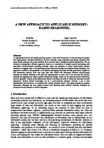
Figure 4.4: Comparison of the times (logarithmic scale) required to prove the property of each benchmark with the previous technique [14] versus our technique. The diagonal line indicates where the tools would have the same performance. The data points in the circle on the right are cases where the previous technique timed out after 4 hours. We have drawn out a set of both ∀CTL and LTL liveness property challenge problems from industrial code bases. Examples were taken from the I/O subsystem of the Windows OS kernel, the back-end infrastructure of the PostgreSQL database server, and the Apache web server. In order to make these examples self-contained we have, by hand, abstracted away the unnecessary functions and struct definitions. We also include a few toy examples, as well as the example from Fig. 8 in [14]. Sources of examples can be found in our technical report [16]. Heap commands from the original sources have been abstracted away using the approach due to Magill et al. [27]. This abstraction introduces new arithmetic variables that track the sizes of recursive predicates found as a byproduct of a successful memory safety analysis using an abstract domain based on separation logic [30]. Support for variables that range over the natural numbers is crucial for this abstraction. As previous mentioned in Section 1.1, there are several available tools for verifying state-based properties of general purpose (infinite-state) programs. Neither the authors of this paper, nor the developer of Yasm [24] were able to apply Yasm to the challenge problems in a meaningful way, due to bugs in the tool. Note that we expect Yasm would have failed in many cases [23], as it is primarily designed to work for unnested existential properties (e.g. EGp or EFp). We have also implemented the approach due to Chaki et al. [9]. The difficulty with applying this approach to the challenge problems is that the programs must first be abstracted to finite-state before branching-time proof methods are applied. Because the challenge problems focus on liveness, we have used transition predicate abstraction [33] as the abstraction method. However, because abstraction must 34

happen first, predicates must be chosen ahead of time either by hand or using heuristics. In practice we found that our heuristics for choosing an abstraction a priori could not be easily tuned to lead to useful results. Because the examples are infinite-state systems, popular CTL-proving tools such as Cadence SMV [1] or NuSMV [10] are not directly applicable. When applied to finite instantiations of the programs these tools run out of memory. The tool described in Cook et al. [14] can be used to prove LTL properties if used in combination with an LTL to B¨ uchi automata conversion tool (e.g. [22]). To compare our approach to this tool we have used two sets of experiments: Fig. 4.2 displays the results on challenge problems in ∀CTL verification; Fig. 4.3 contains results on LTL verification. Experiments were run using Windows Vista and an Intel 2.66GHz processor. In both figures, the code example is given in the first column, and a note as to whether it contains a bug. We also give a count of the lines of code and the shape of the temporal property where p and q are atomic propositions specific to the program. For both the tools we report the total time (in seconds) and the result for each of the benchmarks. A ✓ indicates that a tool proved the property, and χ is used to denote cases where bugs were found (and a counterexample returned). In the case that a tool exceeded the timeout threshold of 4 hours, “>14400.00” is used to represent the time, and the result is listed as “???”. When comparing approaches on ∀CTL properties (Fig. 4.2) we have chosen properties that are equivalent in ∀CTL and LTL and then directly compared our procedure (Algorithm 2.2) to the tool in Cook et al. [14]. When comparing approaches on LTL verification problems (Fig. 4.3) we have used an iterative symbolic determinization strategy [15] which calls our Algorithm 2.2 on successively refined ∀CTL verification problems. The number of such iterations is given as column “#.” in Fig. 4.3. For example, in the case of benchmark Windows OS 3, our procedure was called twice while attempting to prove a property of the form FGp. A visual comparison is given in Figure 4.4. Using a logarithmic scale, we compare the times required to prove the property of each benchmark with the previous technique [14] (on the x-axis) versus our technique (on the y-axis). Our tool is superior whenever a benchmark falls in the bottom-right half of the plot. Timeouts are plotted at 10,000s (seen in the circled area to the right) though they may have run much longer if we had not stopped them. Our technique was able to prove or disprove all but one example, usually in a fraction of a minute. The competing tool fails on over 25% of the benchmarks.

35

Chapter 5 Conclusions We have introduced a novel temporal reasoning technique for (potentially infinite-state) transition systems, with an implementation designed for systems described as programs. Our approach shifts the task of temporal reasoning to a program analysis problem. When an analysis is performed on the output of our encoding, it is effectively reasoning about the temporal and possibly branching behaviors of the original system. Consequently, we can use the wide variety of efficient program analysis tools to prove properties of programs. We have demonstrated the practical viability of the approach using industrial code fragments drawn from the PostgreSQL database server, the Apache web server, and the Windows OS kernel. Acknowledgments. We would like to thank Josh Berdine, Matko Botinˇcan, Michael Greenberg, Daniel Kroening, Axel Legay, Rupak Majumdar, Peter O’Hearn, Joel Ouaknine, Matthew Parkinson, Nir Piterman, Andreas Podelski, Noam Rinetzky, and Hongseok Yang for valuable discussions regarding this work. We also thank the Gates Cambridge Trust for funding Eric Koskinen’s Ph.D. degree program.

36

Bibliography [1] Cadence SMV. http://www.kenmcmil.com/smv.html. [2] Ball, T., Bounimova, E., Cook, B., Levin, V., Lichtenberg, J., McGarvey, C., Ondrusek, B., Rajamani, S. K., and Ustuner, A. Thorough static analysis of device drivers. In EuroSys (2006), pp. 73–85. [3] Berdine, J., Chawdhary, A., Cook, B., Distefano, D., and O’Hearn, P. W. Variance analyses from invariance analyses. In POPL (2007), pp. 211–224. [4] Bernholtz, O., Vardi, M. Y., and Wolper, P. An automata-theoretic approach to branchingtime model checking (extended abstract). In CAV (1994), pp. 142–155. ´, A., Monniaux, [5] Blanchet, B., Cousot, P., Cousot, R., Feret, J., Mauborgne, L., Mine D., and Rival, X. A static analyzer for large safety-critical software. In PLDI (2003), pp. 196–207. [6] Bradley, A., Manna, Z., and Sipma, H. The polyranking principle. Automata, Languages and Programming (2005), 1349–1361. [7] Burch, J., Clarke, E., et al. Symbolic model checking: 1020 states and beyond. Information and computation 98, 2 (1992), 142–170. [8] Calcagno, C., Distefano, D., O’Hearn, P., and Yang, H. Compositional shape analysis by means of bi-abduction. In POPL (2009), pp. 289–300. [9] Chaki, S., Clarke, E. M., Grumberg, O., Ouaknine, J., Sharygina, N., Touili, T., and Veith, H. State/event software verification for branching-time specifications. In IFM (2005), pp. 53–69. [10] Cimatti, A., Clarke, E., Giunchiglia, E., Giunchiglia, F., Pistore, M., Roveri, M., Sebastiani, R., and Tacchella, A. Nusmv 2: An opensource tool for symbolic model checking. In CAV (2002), pp. 241–268. [11] Clarke, E., Emerson, E., and Sistla, A. Automatic verification of finite-state concurrent systems using temporal logic specifications. TOPLAS 8, 2 (1986), 263. [12] Clarke, E., Grumberg, O., and Peled, D. Model checking. 1999. [13] Clarke, E., Jha, S., Lu, Y., and Veith, H. Tree-like counterexamples in model checking. In LICS (2002), pp. 19–29. [14] Cook, B., Gotsman, A., Podelski, A., Rybalchenko, A., and Vardi, M. Y. Proving that programs eventually do something good. In POPL (2007), pp. 265–276. [15] Cook, B., and Koskinen, E. Making prophecies with decision predicates. In POPL (2011), pp. 399–410. [16] Cook, B., Koskinen, E., and Vardi, M. Branching-time reasoning for programs. Tech. Rep. UCAM-CL-TR-788, University of Cambridge, Computer Laboratory, Jan. 2011. [17] Cook, B., Koskinen, E., and Vardi, M. Y. Temporal property verification as a program analysis task. In CAV (2011), G. Gopalakrishnan and S. Qadeer, Eds., vol. 6806 of Lecture Notes in Computer Science, Springer, pp. 333–348.

37

[18] Cook, B., Podelski, A., and Rybalchenko, A. Termination proofs for systems code. In PLDI (2006), pp. 415–426. [19] Delzanno, G., and Podelski, A. Model checking in CLP. TACAS (1999), 223–239. [20] Emerson, E., and Namjoshi, K. Automatic verification of parameterized synchronous systems. In CAV (1996), pp. 87–98. [21] Fioravanti, F., Pettorossi, A., Proietti, M., and Senni, V. Program specialization for verifying infinite state systems: An experimental evaluation. In LOPSTR’10 (2010). [22] Gastin, P., and Oddoux, D. Fast LTL to B¨ uchi automata translation. In CAV (July 2001). [23] Gurfinkel, A. Personal communication. 2010. [24] Gurfinkel, A., Wei, O., and Chechik, M. Yasm: A software model-checker for verification and refutation. In CAV (2006), pp. 170–174. [25] Henzinger, T. A., Jhala, R., Majumdar, R., Necula, G. C., Sutre, G., and Weimer, W. Temporal-safety proofs for systems code. In CAV (2002), pp. 526–538. [26] Kupferman, O., Vardi, M., and Wolper, P. An automata-theoretic approach to branchingtime model checking. J. ACM 47, 2 (2000), 312–360. [27] Magill, S., Berdine, J., Clarke, E., and Cook, B. Arithmetic strengthening for shape analysis. In SAS (2007), vol. 4634, p. 419. [28] Manna, Z., and Pnueli, A. Temporal verification of reactive systems: safety, vol. 2. Springer Verlag, 1995. [29] McMillan, K. Lazy abstraction with interpolants. In CAV (2006), pp. 123–136. [30] O’Hearn, P., Reynolds, J., and Yang, H. Local reasoning about programs that alter data structures. In Computer Science Logic (2001), pp. 1–19. [31] Podelski, A., and Rybalchenko, A. A Complete Method for the Synthesis of Linear Ranking Functions. In VMCAI (2004), pp. 239–251. [32] Podelski, A., and Rybalchenko, A. Transition invariants. In LICS (2004), pp. 32–41. [33] Podelski, A., and Rybalchenko, A. Transition predicate abstraction and fair termination. In POPL (2005). [34] Reps, T., Horwitz, S., and Sagiv, M. Precise interprocedural dataflow analysis via graph reachability. In POPL (1995), pp. 49–61. [35] Schmidt, D., and Steffen, B. Program analysis as model checking of abstract interpretations. Static Analysis (1998), 351–380. [36] Stirling, C. Games and modal mu-calculus. In TACAS (1996), pp. 298–312. [37] Vardi, M. Y. An automata-theoretic approach to linear temporal logic. In Banff Higher Order Workshop (1995), pp. 238–266. [38] Walukiewicz, I. Pushdown processes: Games and model checking. In CAV (1996), pp. 62–74. [39] Walukiewicz, I. Model checking CTL properties of pushdown systems. FST TCS (2000), 127–138.

38