Breakdown of the generalized Gibbs ensemble for current-generating ...

Breakdown of the generalized Gibbs ensemble for current–generating quenches Marcin Mierzejewski,1 Peter Prelovˇsek,2, 3 and Tomaˇz Prosen2

arXiv:1405.2557v1 [cond-mat.str-el] 11 May 2014

2

1 Institute of Physics, University of Silesia, 40-007 Katowice, Poland Faculty of Mathematics and Physics, University of Ljubljana, SI-1000 Ljubljana, Slovenia 3 J. Stefan Institute, SI-1000 Ljubljana, Slovenia

We establish a relation between two hallmarks of integrable systems: the relaxation towards the generalized Gibbs ensemble (GGE) and the dissipationless charge transport. We show that the former one is possible only if the so called Mazur bound on the charge stiffness is saturated by local conserved quantities. As an example we show how a non–GGE steady state with a current can be generated in the one-dimensional model of interacting spinless fermions with a flux quench. Moreover an extended GGE involving the quasi-local conserved quantities can be formulated for this case. PACS numbers: 72.10.-d,75.10.Pq, 05.60.Gg,05.70.Ln

Recent advances in experiments on ultracold atoms together with new computational techniques have significantly broadened our understanding of relaxation processes in closed many-body quantum systems. It is commonly accepted that in generic macroscopic systems the long–time averages of local observables coincide with the results for the statistical Gibbs ensemble [1–4] and are uniquely determined by few parameters related to conserved quantities, in particular the system’s energy and particle number. Due to the presence of macroscopic number of conserved quantities such a simple scenario is not applicable to integrable systems [5–7]. However, there is a large and still growing evidence that relaxation in the latter systems is consistent with the generalized Gibbs ensemble (GGE) [8–12], where the density matrix is determined not only by the Hamiltonian H and particle number N but also by other local conserved quantities P Qi , i.e., ρGGE ∼ exp [−β(H − µN ) − i λi Qi ]. In this Letter we focus on the relaxation dynamics of one of the most studied integrable models: the model of interacting spinless fermions, being equivalent to the anisotropic Heisenberg (XXZ) model for which the set of Qi has been established [13, 14]. We show that ρGGE as generated only by local integrals of motion Qi doesn’t exhaust all generic stationary states in the metallic (easy plane) regime. Instead, there are cases for which one should lift the requirement of locality of the conserved quantities and allow also for quasi–local integrals of motion [15, 16]. In this Letter we call them non–GGE states, however we stress that these states can be viewed also as “extended GGE”, where the extension concerns the locality of operators. Such operators have the parity opposite to local ones Qi . We identify one of such quasi–local quantities as the time–averaged particle current operator and we construct as well as verify it explicitly. It has been well recognized that integrable systems in spite of interaction reveal anomalous transport properties at finite inverse temperatures β = 1/T , e.g. the dissipationless particle current. This property is manifested by a nonvanishing charge stiffness D(β < ∞) [17–19], which

in turn is bounded from below by the local conservation laws via the Mazur bound [18, 20]. The dissipationless transport and the relaxation towards GGE are probably the most prominent hallmarks of integrability, still they have been studied independently of each other so far. While it has been clear that in certain regimes the standard Mazur bound with only local Qi does not exhaust the phenomenon of dissipationless transport and D(β < ∞) > 0 [18] we show in this Letter that GGE should be extended by taking into account quasi–local conserved quantities of different parity, in particular the time averaged current, which saturate D(β → ∞) within the Mazur bound. We study a prototype one-dimensional (1D) model of interacting particles, the tight-binding model of spinless fermions on L sites at half filling (with N = L/2 particles) and with periodic boundary conditions [21–24], H(t) = −th

L L X X (eiφ(t) c†j+1 cj + h.c.) + V n ˜j n ˜ j+1 , (1) j=1

j=1

where nj = c†j cj , n ˜ j = nj −1/2, th is the hopping integral and V is the repulsive interaction on nearest neighbors. The model (1) is equivalent to the anisotropic Heisenberg (XXZ) model with the exchange interaction J = 2th and the anisotropy parameter ∆ = V /2th . However, we stay within the fermionic representation, where the phase φ(t) has a clear physical meaning: it represents the timedependent magnetic flux which induces the electric field F (t) = −∂t φ(t). Further on we use h ¯ = kB = 1 and units in which th = 1. We consider here the metallic (easy– plane) regime V < 2 (∆ < 1) where the system exhibits a ballistic particle (spin) transport at T > 0 [17–19, 25–32]. The charge stiffness D(T ) > 0 has been introduced via the T > 0 generalization of the Kohn’s [33] argument of the level curvatures n (φ) [17, 34]. It is still a challenging problem since it cannot be derived from local conservation laws [18, 35]. To explore this relation we study P in the following the standard particle current J = j (ieiφ(t) c†j+1 cj + h.c.) as well a less common cur-

2 0.16

where ρ¯o and ρ¯e are odd and even under the transformation (2), respectively. Since Tr{¯ ρJ} = Tr{¯ ρo J} the odd component of the density matrix ρ¯o is essential for the nonvanishing current hJ(t > 0)i, while this component is missing in ρGGE . At this stage it is instructive to recall the linear–response (LR) results Z ∞ hJ(t)i = L dωe−iωt F (ω)σ(ω), (4)

0.7

4

0.14

4

0.6

0.12

0.5

0.1

0.4

0.08

0.3

0.06

0.2

0.04

a)

0.02 0

10

20 t 30

b)

0.1

0 40

50

0 0

10

20

t

30

40

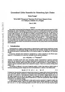
FIG. 1. (Color online) Time–dependence of hJi and 4hJ 0 i after quenching the flux at t = 0 for L = 26 and V = 1. a) The system is initially in equilibrium microcanonical state with β = 0.35 while after the quench it has effective β = 0.15. b) The system is in the ground state and the flux is quenched from φ0 = π/2 to 0.

rent with P a correlated hopping to next-nearest neighbors J 0 = j (ie2iφ(t) c†j+2 n ˜ j+1 cj + h.c.). The central point in our reasoning is the particle–hole (parity) transformation ci → (−1)i c†i ,

−∞

50

(2)

which (for φ = 0) does not alter the Hamiltonian H → H (at half filling) nor the local conserved quantities Qi → Qi [18] but reverses the currents J → −J and J 0 → −J 0 , hence J(J 0 ) and Qi have different parities. We start with numerical studies of a quantum quench which generates a non–GGE steady state. We consider a system which for t < 0 is either in the ground state or in the equilibrium canonical or microcanonical state [36]. In the latter case we generate a state ρ(0) = |Ψ(0)ihΨ(0)| for the target energy E0 = hΨ(0)|H(0)|Ψ(0)i and with a small energy uncertainty δ 2 E0 = hΨ(0)|[H(0) − E0 ]2 |Ψ(0)i as discussed in Refs. [37, 38]. The time– evolution shown in Fig. 1 has been obtained by the Lanczos propagation method [37–39]. At t = 0 the magnetic flux is suddenly decreased from the initial value φ(0) = φ0 > 0 to φ(t > 0) = 0. Such a quench is equivalent to a pulse of the electric field F (t) = φ0 δ(t) hence it generates the particle current 6= 0. As shown in Fig. 1 this quench induces also hJ 0 (t)i 6= 0, however the latter quantity increases gradually in contrast to the instantaneous generation of hJ(t > 0)i. Both currents reach for t → ∞ finite steady values, clearly visible in Fig. 1, being the signature of dissipationless transport. Still the residual values hJi = 6 0 and hJ 0 i 6= 0 cannot be explained within the GGE– scenario since Tr{ρGGE J} = Tr{ρGGE J 0 } = 0 due to different symmetries under particle–hole transformation at half filling [18]. The first objective of this Letter is to establish the symmetry decomposed time averaged density matrix Z 1 τ dtρ(t) = ρ¯e + ρ¯o , (3) ρ¯ = lim τ →∞ τ 0

where the optical conductivity σ(ω) consists of the regular and the ballistic parts with the latter one determined by the charge stiffness D: σbal (ω) = 2Di/(ω + i0+ ). The quench of flux induces an electric field F (ω) = φ0 /(2π) and the regular (dissipative) part of conductivity becomes irrelevant in the long–time regime. Then we get within the LR, i.e. for φ0  1, lim hJ(t)i = 2LDφ0 .

(5)

t→∞

An important message following from LR, Eq.(5), is that the non–GGE component of the density matrix has to contain contributions which are linear in φ0 and, therefore, can be singled out already within the first–order perturbation expansion in φ0 . The unperturbed Hamiltonian H0 = H(t < 0) is given by Eq. (1) with φ(t) replaced by φ0 , while the perturbation reads H 0 (t) = H(t) − H0 = (φ0 − φ(t))J0 , where J0 = J(t < 0), so that H 0 (t > 0) = φ0 J0 . For the sake of clarity all quantities obtained with the flux φ0 will be marked with a label ”0”, in particular the eigenvalues Em0 and the eigenvectors |m0i of H0 . The degeneracy of energy levels plays an important role and should not be neglected. Hence, we diagonalize the current operator in each subspace spanned by degenerate eigenstates and take the eigenvectors of J as the basis vectors of this subspace, i.e., hm|J|ni ∝ δmn if Em = En (within a subspace only). We assume that the Psystem is initially in a thermal sate, i.e. ρ0 = m pm0 |m0ihm0| with pm0 = exp(−βEm0 )/Z0 . Then, in the Schr¨odinger picture one obtains X pm0 e−iH0 t U (t)|m0ihm0|U † (t)eiH0 t , ρ(t > 0) = m



Z

U (t > 0) = Tt exp −i

t 0

dt



HI0 (t0 )

,

(6)

0

where HI0 (t0 ) is the perturbation in the interaction picture. Our aim is to explicitly express ρ¯ within the LR to the quench φ0 . A straightforward calculation of Eqs. (3),(6) to first order in φ0 yields X pn0 − pm0 hm0|J0 |n0i|m0ihn0|. ρ¯ ' ρ0 + φ0 En0 − Em0 Em0 6=En0

(7) We should also take into account the change of current operator due to flux, hence J = J(t > 0) = J0 − φ0 H0k ,

(8)

3 where H0k is the kinetic part of H0 , Eq. (1). Using Eqs. (7),(8),(5) one then restores the LR result for the equilibrium charge stiffness [17, 34]   X p − p 1  m0 n0 −hH0k i + |hm0|J0 |n0i|2  . D= 2L Em0 − En0 Em0 6=En0

(9) Eq. (7) does not yet accomplish our aim of decomposing ρ¯ into odd and even parts with respect to (2) after the quench φ(t > 0) = 0. We achieve this by using again the first–order perturbation theory for H0 = H − φ0 J and J0 = J + φ0 H k , where now H, H k and J are the operators after the quench, i.e. at φ = 0. Substituting En0 = En − φ0 hn|J|ni, X |n0i = |ni − φ0 m:Em 6=En

hm|J|ni |mi, En − Em

(10)

n

where J¯ is the time-averaged steady–current operator Z X 1 τ hn|J|ni|nihn|. (12) J¯ = lim dteiHt Je−iHt = τ →∞ τ 0 n The LR results [Eq. (5)] is immediately restored, however this time with the alternative form of the charge stiffness but equivalent for β < ∞ and in the thermodynamic limit [18] β X pn hn|J|ni2 . 2L n

(13)

¯ = 0. It is By definition J¯ is an integral of motion [H, J] 2 ¯ important to note that TrJ /N ∝ L where N = Tr 1 is the dimension of the Hilbert space, already implies that J¯ is a quasi–local quantity. Since at β → 0, 1 ˜ TrJ¯2 = 2LD, N

where

˜ = lim D(β)/β, D β→0

(14)

the quasi-local character of J¯ is consistent with the well established fact that the charge stiffness is an intensive quantity. We now turn to the question of whether ρ¯ is compatible with ρGGE and the answer is clearly negative. A necessary and a sufficient condition for such compatibility, to leading order in the quench φ0 , would be a decomposition in terms of local conserved Qi , X J¯ = αi Qi , (15) i

i

which holds for any ai and becomes an equality only for the GGE state with ai = αi . Now we can follow original steps by Mazur [20]. We minimize the lhs of Eq. (16) with respect to ai , ai =

¯ i} Tr{JQi } Tr{JQ = , 2 Tr{Qi } Tr{Q2i }

(17)

and substitute this result in (16) to obtain the Mazur inequality for β → 0 Tr{J¯2 } ≥

X Tr{JQi }2 i

into Eq. (7), and assuming that there is no particle current in the initial thermal state, we finally obtain X
ρ¯ = pn |nihn| 1 + βφ0 J¯ , (11)

D=

holding for some set of αi . Assuming that Tr{Qi Qj } ∝ δij we can employ the inequality X Tr{(J¯ − ai Qi )2 } ≥ 0, (16)

Tr{Q2i }

,

(18)

which is the Mazur bound on charge stiffness at T → ∞ [see Eq. (14)]. Since this inequality turns into equality for GGE states, so should the Mazur bound. In other words relaxation towards GGE is possible provided the Mazur bound saturates the charge stiffness.This relation holds for an arbitrary filling N/L. In particular for N/L = 1/2 one finds Tr(Qi J) = 0 due to the symmetry (2), hence the rhs of (18) vanishes, and our quenched dynamics does not relax to GGE. As has been shown in Refs. [15, 16], another set of non-local, but quasi-local conserved Hermitian operators {Q(ϕ)} exists for a dense set commensurate interactions ∆ = cos(πl/m), with l, m integers, densely covering the range |V | < 2. They are all odd under (2), Q(ϕ) → −Q(ϕ). Quasi-locality implies linear extensivity Tr{Q(ϕ)2 }/N ∝ L, similarly as for the local conserved operators Qi , while Tr{JQ(ϕ)}/(LN ) = const, making them suitable for implementing the Mazur bound. For ∆ = cos(π/m) for which T → ∞ limit of the Bethe ansatz result [25] is available it has been shown [16] to agree precisely with the Mazur bound, so one may conjecture that the latter is now indeed saturated. Hence our argument (15-18) can be used to argue that the complete time-averaged current can be expressed in terms of an integral Z J¯ = d2 ϕf (ϕ)Q(ϕ) (19) Dm

where f (ϕ) = cm /| sin ϕ|4 for a suitable constant cm (see [16]) and Dm is a vertical strip in the complex plane with |Reϕ − π/2| < π/(2m). After straightforward calculation, again using the notation and machinery of [16], one arrives at the explicit matrix-product expression for † J¯ = i(J+ − J+ ) in terms of local operators X X (r) J+ = Jj (20) j

r≥2

4 with

0.12 s

r−1 + gs2 ...sr−1 (B s2 · · · B sr−1 )11 σ1− σ2s2 · · · σr−1 σr ,

s2 ,...,sr−1 #+ {si } 

gs2 ,...,sr−1 :=

X j=0

0.1 D’/D

=

0.09

a)

0.08

 #+ {si } Ij+ 12 #z {si } j

0.07

(21)

0.06 0.05

where #s {si } denotes the numberR of indices in the set {si } having a value s. Here Ik := Dm d2 ϕf (ϕ)(cot ϕ)2k are elementary integrals which can be evaluated as 2k+1 X 2k + 1 2π (−1)j × Ik = − m(2k + 1)(sin π/m)2k+2 j=0 j (cos π/m)2k+1−j (sinc(π(j + 1)/m) − sinc(π(j − 1)/m)) , and Ik+1/2 = 0 for k integer. The coefficient of Eq. (21) (B s2 · · · B sr−1 )11 is the (1, 1)-component of a product of (m − 1) × (m − 1) matrices B s , related to modified Lax operator [16], 0 Bj,k = cos(πjl/m)δj,k ,

z Bj,k = − sin(πjl/m)δj,k , (22)

− Bj,k = sin(πkl/m)δj+1,k ,

+ Bj,k = − sin(πjl/m)δj,k+1 .

Pauli matrices σjs are related to fermion operators via Qj−1 Jordan-Wigner transformation cj = ( i=1 σiz )σj− . The result (21) is derived in the limit L → ∞ and is valid up to corrections of order O(1/L) for a finite periodic ring. Explicitly, J¯ to all terms up to order four (r ≤ 4) reads X † ˜ (8J + 2V J 0 ) + J¯ = D iκcj+3 cj + iκ0 c†j+3 c†j+2 cj+1 cj j

+iκ00 c†j+3 n ˜ j+2 n ˜ j+1 cj

 + h.c. + . . .

(23)

For example, for V = 1, (∆ = cos π3 ), one has explicitly √ √ √ 1 3 3 1 9 3 9 3 0 ˜ D= − , κ= − , κ = − 1, (24) 8 32π 4 16π 8π ˜ 2 /16 in general. while κ00 = DV Above analytical results are nicely corroborated by exact numerical simulations in finite systems shown in Fig. 2. From Eq. (23) one finds that the ratio of two currents should be given as Tr{¯ ρJ 0 }/Tr{¯ ρJ} = V /4 as confirmed in Fig. 2b. Furthermore, one can define the 2 stiffness with respect to current J 0 as D0 = hβJ 0 i/(2L). ¯ Formula (23) immediately implies that J 0 = (V /4)J, and so the two stiffnesses should have a simple ratio D0 /D = (V /4)2 (see Fig. 2a). In conclusion, we have proposed a class of global quantum quench dynamics of integrable spin chains for which the state at asymptotic times does not relax to GGE. We argue that, at least for weak quenches where linear response theory is applicable, the validity of GGE ensemble is in one-to-one correspondence with the saturation of the Mazur bound expressed in terms of strictly local

0

0.02

0.04

0.06 1/L

0.08

0.1

0.25 /

(r)

J1

X

data fit 1/16

0.11

{0,z,±}

0.24 0.23

b)

0.22 data fit 1/4

0.21 0.2 0

0.02

0.04

0.06

0.08

0.1

1/L

FIG. 2. (Color online) a) D0 /D vs. 1/L, where D0 is the stiffness related with J 0 . b) hJi/hJ 0 i obtained for ρ¯, Eq.(11), for β → 0. Horizontal lines show analytical results. Exact diagonalization has been carried out for V = 1 with φ = π/L and 2π/L for even and odd N , respectively.

conserved operators. However, if one extends the GGE ensemble by including the quasi-local conserved operators from the opposite parity sector – having linearly extensive Hilbert-Schmidt norm – then the latter can be used to describe exactly the steady state density operator after the quench. Our theory has been demonstrated in the 1D model of interacting spinless fermions (XXZ spin model) within the metallic regime. It should be noted that our results are expected to have further implications on other relevant quantities of integrable system besides the charge stiffness. The flux– ¯ = 2 P sin(k)h¯ quench induced steady current hJi nk i 6 = k 0 is reflected into the fermion momentum–distribution function h¯ nk i which also does not comply to the standard GGE. The latter quantity is the one typically measured in cold–atom experiments [40, 41] as well most frequently studied in connection with the GGE concept [5, 8, 10]. The inclusion of the quasi–local conserved quantity J¯ fully fixes the steady state h¯ nk i within our quench protocol via extended GGE form Eq. (11). It is still tempting to construct and consider further (presumably conserved) quantities from the same polarity sector which would fix this and related quantities for an arbitrary quench. M.M. acknowledges support from the NCN project DEC-2013/09/B/ST3/01659. P.P. and T.P. acknowledges the support by the program P1-0044 and projects J1-4244 (P. P.) and J1-5349 (T. P.) of the Slovenian Research Agency.

5

[1] S. Goldstein, J. L. Lebowitz, R. Tumulka, and N. Zangh`ı, Phys. Rev. Lett. 96, 050403 (2006). [2] N. Linden, S. Popescu, A. J. Short, and A. Winter, Phys. Rev. E 79, 061103 (2009). [3] A. Riera, C. Gogolin, and J. Eisert, Phys. Rev. Lett. 108, 080402 (2012). [4] A. Polkovnikov, K. Sengupta, A. Silva, and M. Vengalattore, Rev. Mod. Phys. 83, 863 (2011). [5] S. R. Manmana, S. Wessel, R. M. Noack, and A. Muramatsu, Phys. Rev. Lett. 98, 210405 (2007). [6] L. F. Santos, A. Polkovnikov, and M. Rigol, Phys. Rev. Lett. 107, 040601 (2011). [7] M. Mierzejewski, T. Prosen, D. Crivelli, and P. Prelovˇsek, Phys. Rev. Lett. 110, 200602 (2013). [8] M. Rigol, V. Dunjko, V. Yurovsky, and M. Olshanii, Phys. Rev. Lett. 98, 050405 (2007). [9] M. Kollar, F. A. Wolf, and M. Eckstein, Phys. Rev. B 84, 054304 (2011). [10] A. C. Cassidy, C. W. Clark, and M. Rigol, Phys. Rev. Lett. 106, 140405 (2011). [11] C. Gogolin, M. P. M¨ uller, and J. Eisert, Phys. Rev. Lett. 106, 040401 (2011). [12] M. Fagotti, M. Collura, F. H. L. Essler, and P. Calabrese, Phys. Rev. B 89, 125101 (2014). [13] M. Tetelman, Sov. Phys. JETP 55, 306 (1982). [14] M. P. Grabowski and P. Mathieu, Ann. Phys. (N.Y.) 243, 299 (1995). [15] T. Prosen, Phys. Rev. Lett. 106, 217206 (2011). [16] T. Prosen and E. Ilievski, Phys. Rev. Lett. 111, 057203 (2013). [17] X. Zotos and P. Prelovˇsek, Phys. Rev. B 53, 983 (1996). [18] X. Zotos, F. Naef, and P. Prelovsek, Phys. Rev. B 55, 11029 (1997). [19] R. Steinigeweg, J. Gemmer, and W. Brenig, Phys. Rev. Lett. 112, 120601 (2014). [20] P. Mazur, Physica 43, 533 (1969). [21] M. B¨ uttiker, Y. Imry, and R. Landauer, Physics Letters A 96, 365 (1983).

[22] G. Blatter and D. A. Browne, Phys. Rev. B 37, 3856 (1988). [23] R. H¨ ubner and R. Graham, Phys. Rev. B 53, 4870 (1996). [24] R. Landauer and M. B¨ uttiker, Phys. Rev. Lett. 54, 2049 (1985). [25] X. Zotos, Phys. Rev. Lett. 82, 1764 (1999); J. Benz, T. Fukui, A. Kl¨ umper, and C. Scheeren, Journal of the Physical Society of Japan 74, 181 (2005), http://journals.jps.jp/doi/pdf/10.1143/JPSJS.74S.181. [26] F. Heidrich-Meisner, A. Honecker, and W. Brenig, The European Physical Journal Special Topics 151, 135 (2007). [27] M. Rigol and B. S. Shastry, Phys. Rev. B 77, 161101 (2008). [28] J. Herbrych, P. Prelovˇsek, and X. Zotos, Phys. Rev. B 84, 155125 (2011). ˇ [29] M. Znidariˇ c, Phys. Rev. Lett. 106, 220601 (2011). [30] J. Sirker, R. G. Pereira, and I. Affleck, Phys. Rev. Lett. 103, 216602 (2009). [31] T. Prosen, Phys. Rev. Lett. 107, 137201 (2011). [32] R. Steinigeweg, J. Herbrych, P. Prelovˇsek, and M. Mierzejewski, Phys. Rev. B 85, 214409 (2012). [33] W. Kohn, Phys. Rev. 133, A171 (1964). [34] H. Castella, X. Zotos, and P. Prelovˇsek, Phys. Rev. Lett. 74, 972 (1995). [35] M. Hawkins, M. Long, and X. Zotos, arXiv:0812.3096v1 . [36] M. W. Long, P. Prelovˇsek, S. El Shawish, J. Karadamoglou, and X. Zotos, Phys. Rev. B 68, 235106 (2003). [37] M. Mierzejewski and P. Prelovˇsek, Phys. Rev. Lett. 105, 186405 (2010). [38] M. Mierzejewski, J. Bonˇca, and P. Prelovˇsek, Phys. Rev. Lett. 107, 126601 (2011). [39] T. J. Park and J. C. Light, The Journal of Chemical Physics 85, 5870 (1986). [40] M. Greiner, O. Mandel, T. Esslinger, T. Hansch, and I. Bloch, Nature 415, 39 (2002). [41] I. Bloch, Nat Phys 1, 23 (2005).