Breaking the Curse of Dimensionality with Convex Neural Networks

B REAKING

THE

C URSE

OF

D IMENSIONALITY

WITH

C ONVEX N EURAL N ETWORKS

Breaking the Curse of Dimensionality with Convex Neural Networks Francis Bach

FRANCIS . BACH @ ENS . FR

arXiv:1412.8690v1 [cs.LG] 30 Dec 2014

INRIA - Sierra Project-team Département d’Informatique de l’Ecole Normale Supérieure Paris, France

Editor:

Abstract We consider neural networks with a single hidden layer and non-decreasing homogeneous activation functions like the rectified linear units. By letting the number of hidden units grow unbounded and using classical non-Euclidean regularization tools on the output weights, we provide a detailed theoretical analysis of their generalization performance, with a study of both the approximation and the estimation errors. We show in particular that they are adaptive to unknown underlying linear structures, such as the dependence on the projection of the input variables onto a low-dimensional subspace. Moreover, when using sparsity-inducing norms on the input weights, we show that high-dimensional non-linear variable selection may be achieved, without any strong assumption regarding the data and with a total number of variables potentially exponential in the number of observations. In addition, we provide a simple geometric interpretation to the non-convex problem of addition of a new unit, which is the core potentially hard computational element in the framework of learning from continuously many basis functions. We provide simple conditions for convex relaxations to achieve the same generalization error bounds, even when constant-factor approximations cannot be found (e.g., because it is NP-hard such as for the zero-homogeneous activation function). We were not able to find strong enough convex relaxations and leave open the existence or non-existence of polynomial-time algorithms. Keywords: Neural networks, non-parametric estimation, convex optimization, convex relaxation

1. Introduction Supervised learning methods come in a variety of ways. They are typically based on local averaging methods, such as k-nearest neighbors, decision trees, or random forests, or on optimization of the empirical risk over a certain function class, such as least-squares regression, logistic regression or support vector machine, with positive definite kernels, with model selection, structured sparsity-inducing regularization, or boosting (see, e.g., Györfi and Krzyzak, 2002; Hastie et al., 2009; Shalev-Shwartz and Ben-David, 2014, and references therein). Most methods assume either explicitly or implicitly a certain class of models to learn from. In the non-parametric setting, the learning algorithms may adapt the complexity of the models as the number of observations increases: the sample complexity (i.e., the number of observations) to adapt to any particular problem is typically large. For example, when learning Lipschitz-continuous functions in Rd , at least n = Ω(ε− max{d,2} ) samples are needed to learn a function with excess risk ε (von Luxburg and Bousquet, 2004). The exponential dependence on the dimension d is often 1

BACH

referred to as the curse of dimensionality: without any restrictions, exponentially many observations are needed to obtain optimal generalization performances. At the other end of the spectrum, parametric methods such as linear supervised learning make strong assumptions regarding the problem. The generalization performance will only be optimal if these are met, and the sample complexity to attain an excess risk of ε grows as n = Ω(d/ε2 ), for linear functions in d dimensions and Lipschitz-continuous loss functions. While the sample complexity is much lower, when the assumptions are not met, the methods underfit and more complex models would provide better generalization performances. Between these two extremes, there are a variety of models with structural assumptions that are often used in practice. For input data in x ∈ Rd , prediction functions f : Rd → R may for example be parameterized as: (a) Affine functions: f (x) = w⊤ x + b, leading to potential severe underfitting, but easy optimization and good (i.e., non exponential) sample complexity. P (b) Generalized additive models: f (x) = dj=1 fj (xj ), which are generalizations of the above by summing functions fj : R → R which may not be affine (Hastie and Tibshirani, 1990; Ravikumar et al., 2008; Bach, 2008a). This leads to less strong underfitting but cannot model interactions between variables, while the estimation may be done with similar tools than for affine functions (e.g., convex optimization for convex losses). P (c) Nonparametric ANOVA models: f (x) = A∈A fA (xA ) for a set A of subsets of {1, . . . , d}, and non-linear functions fA : RA → R. The set A may be either given (Gu, 2013) or learned from data (Lin and Zhang, 2006; Bach, 2008b). Multi-way interactions are explicitly included but a key algorithmic problem is to explore the 2d − 1 non-trivial potential subsets. P (d) Single hidden-layer neural networks: f (x) = kj=1 σ(wj⊤ x + bj ), where k is the number of units in the hidden layer (see, e.g., Rumelhart et al., 1986; Haykin, 1994). The activation function σ is here assumed to be fixed. While the learning problem may be cast as a (sub)differentiable optimization problem, techniques based on gradient descent may not find the global optimum. If the number of hidden units is fixed, this is a parametric problem. Pk ⊤ (e) Projection pursuit (Friedman and Stuetzle, 1981): f (x) = j=1 fj (wj x) where k is the number of projections. This model combines both (b) and (d); the only difference with neural networks is that the non-linear functions fj : R → R are learned from data. The optimization is often done sequentially and is harder than for neural networks. (e) Dependence on a unknown k-dimensional subspace: f (x) = g(W ⊤ x) with W ∈ Rd×k , where g is a non-linear function. A variety of algorithms exist for this problem (Li, 1991; Fukumizu et al., 2004; Dalalyan et al., 2008). Note that when the columns of W are assumed to be composed of a single non-zero element, this corresponds to variable selection (with at most k selected variables). In this paper, our main aim is to answer the following question: Is there a single learning method that can deal efficiently with all situations above with provable adaptivity? We consider singlehidden-layer neural networks, with non-decreasing homogeneous activation functions such as σ(u) = max{u, 0}α = (u)α+ , 2

B REAKING

THE

C URSE

OF

D IMENSIONALITY

WITH


for α ∈ {0, 1, . . .}, with a particular focus on α = 0, that is σ(u) = 1u>0 (a threshold at zero), and α = 1, that is, σ(u) = max{u, 0} = (u)+ , the so-called rectified linear unit (Nair and Hinton, 2010; Krizhevsky et al., 2012). We follow the convexification approach of Bengio et al. (2006); Rosset et al. (2007), who consider potentially infinitely many units and let a sparsity-inducing norm choose the number of units automatically. We make the following contributions: – We provide in Section 2 a review of functional analysis tools used for learning from continuously infinitely many basis functions, by studying carefully the similarities and differences between L1 - and L2 -penalties on the output weights. – We provide a detailed theoretical analysis of the generalization performance of (single hidden layer) convex neural networks with monotonic homogeneous activation functions, with study of both the approximation and the estimation errors, with explicit bounds on the various needed weights. We relate these new results to the extensive literature on approximation properties of neural networks (see, e.g., Pinkus, 1999, and references therein) in Section 4.7. – In Section 5, we show that these convex neural networks are adaptive to all situations mentioned earlier. When using an ℓ1 -norm on the input weights, we show in Section 5.3 that high-dimensional non-linear variable selection may be achieved, without any strong assumption regarding the data (note that we do not present a polynomial-time algorithm to achieve this). – In Sections 3.2, 3.3 and 3.4, we provide simple geometric interpretations to the non-convex problems of additions of new units, which constitute the core potentially hard computational tasks in our framework of learning from continuously many basis functions. – We provide in Section 5.5 simple conditions for convex relaxations to achieve the same generalization error bounds, even when constant-factor approximation cannot be found (e.g., because it is NP-hard such as for the zero-homogeneous activation function). We were not able to find strong enough convex relaxations and leave open the existence or non-existence of polynomial-time algorithms.

2. Learning from continuously infinitely many basis functions In this section we present the functional analysis framework underpinning the methods presented in this paper. While the formulation from Sections 2.1 and 2.2 originates from the early work on the approximation properties of neural networks (Barron, 1993; Kurkova and Sanguineti, 2001), the algorithmic parts that we present in Section 2.5 have been studied in a variety of contexts, such as “convex neural networks” (Bengio et al., 2006), or ℓ1 -norm with infinite dimensional feature spaces (Rosset et al., 2007), with links with conditional gradient algorithms (Dunn and Harshbarger, 1978; Jaggi, 2013) and boosting (Rosset et al., 2004). In the following sections, note that there will be two orthogonal notions of infinity: infinitely many inputs x and infinitely many basis functions x 7→ ϕv (x). Moreover, two orthogonal notions of Lipschitz-continuity will be tackled in this paper: the one of the prediction functions f , and the one of the loss ℓ used to measure the fit of these prediction functions. 3

BACH

2.1 Variation norm We consider an arbitrary measurable input space X (this will be Rd from Section 3), with a set of basis functions (a.k.a. neurons or units) ϕv : X → R, which are parameterized by v ∈ V, where V is a compact topological space (typically a sphere for a certain norm on Rd starting from Section 3). We assume that for any given x ∈ X , the functions v 7→ ϕv (x) are continuous. In order to define our space of functions from X → R, we need real-valued Radon measures, which are continuous linear forms on the space of continuous functions from V to R, equipped with the uniform norm (Rudin, 1987; Evans and Gariepy, 1991). RFor a continuous function g : V → R and a Radon measure µ, we will use the standard notation V g(v)dµ(v) to denote the action of the measure µ on the continuous function g. The norm of µ is usually R referred to as its total variation, and we denote it as |µ|(V), and is equal to the supremum of V g(v)dµ(v) over all continuous functions with values in [−1, 1]. As seen below, when µ has a density with respect to a probability measure, this is the L1 -norm of the density. We consider the space F1 of functions f that can be written as Z ϕv (x)dµ(v), f (x) = V

where µ is a signed Radon measure on V with finite total variation |µ|(V). When V is finite, this corresponds to X f (x) = µv ϕv (x), v∈V

with total variation measure theory.

P

v∈V

|µv |, where the proper formalization for infinite sets V is done through

R The infimum of |µ|(V) over all decompositions of f as f = V ϕv dµ(v), turns out to be a norm γ1 on F1 , often called the variation norm of f with respect to the set of basis functions (see, e.g., Kurkova and Sanguineti, 2001). Given our assumptions regarding the compactness of V, for any f ∈ F1 , the infimum defining γ1 (f ) is in fact attained by a signed measure µ, as a consequence of the compactness of measures for the weak topology (see Evans and Gariepy, 1991, Section 1.9). In the definition above, if we assume that the signed measure µ has a density with respect to a fixed probability measure τ with full support on V, that is, dµ(v) = p(v)dτ (v), then, the total mass |µ|(V) is equal to the infimal value of Z |p(v)|dτ (v), |µ|(V) = V

R

for decompositions f (x) = V p(v)ϕv (x)dτ (v). Note however that not all measures have densities but that the two infimums are the same as all Radon measures are limits of measures with densities. This implies that the infimum in the definition above is not attained in general; however, it often provides a more intuitive definition of the variation norm. Finite number of neurons. If f : X → R is decomposable into k basis functions, that is, f (x) = P Pk k η ϕ (x), then this corresponds to µ = η δ(v = vj ), and the total variation of µ is j=1 j vj j=1 j 4

B REAKING

THE

C URSE

OF

D IMENSIONALITY

WITH


equal to kηk1 . Thus the function f has variation norm less than kηk1 . This is to be contrasted with the number of basis functions, which is the ℓ0 -pseudo-norm. 2.2 Representation from finitely many functions When minimizing any function J that depends only on a subset Xˆ of values in X over the ball {f ∈ F1 , γ1 (f ) 6 δ}, then we have a “representer theorem”. The problem is indeed simply ˆ equivalent to minimizing J(f|Xˆ ) over f|Xˆ ∈ RX , such that γ1|Xˆ (f|Xˆ ) 6 δ, where Z ˆ ϕv (x)dµ(v). γ1|Xˆ (f|Xˆ ) = inf |µ|(V) such that ∀x ∈ X , f|Xˆ (x) = µ

V

Moreover, by Carathéodory’s theorem for cones (Rockafellar, 1997), if Xˆ is composed of only n elements, as often in machine learning, f (and hence f|Xˆ ) may be decomposed into at most n functions ϕv , that is, µ is supported by at most n points. Note that these n functions are not known in advance, and thus there is a significant difference with the representer theorem for positive definite kernels (see, e.g., Shawe-Taylor and Cristianini, 2004), where the set of n functions are known from the knowledge of the points x ∈ Xˆ (i.e., kernel functions evaluated at x). 2.3 Corresponding reproducing kernel Hilbert space (RKHS) We have seen above that if the real-valued measures µ have density p with respect to a fixed probability measure τ with full support on V, that R is, dµ(v) = p(v)dτ (v), then, the norm γ1 (f ) is the infimum of the total variation |µ|(V) = V |p(v)|dτ (v), over all decompositions f (x) = R p(v)ϕ (x)dτ (v). v V R We may also define the infimum of V |p(v)|2 dτ (v) over the same decompositions (squared L2 norm instead of L1 -norm). It turns out that it defines a squared norm and that the function space of functions with finite norms happens to be a reproducing kernel Hilbert space (RKHS). When V 2004, Section 4.1) that the is finite, then (see, e.g., Berlinet and Thomas-Agnan, P Pit is well-known 2 infimum of v∈V µv over all vectors µPsuch that f = v∈V µv ϕv defines a squared RKHS norm with positive definite kernel k(x, y) = v∈V ϕv (x)ϕv (y). 2 We show in Appendix A that for any Z compact V, we have defined a squared RKHS norm γ2 with ϕv (x)ϕv (y)dτ (v). positive definite kernel k(x, y) = V

Random sampling. Note that such kernels are well-adapted to approximations by sampling several basis functions ϕv sampled from the probability measure τ (Neal, 1995; Rahimi and Recht, 2007). Indeed, if we consider m i.i.d. samples v1 , . . . , vm , we may define the approximation 1 Pm ˆ In other k(x, y) = m i=1 ϕvi (x)ϕvi (y), which corresponds to an explicit feature representation. 1 Pm words, this corresponds to sampling units vi , using prediction functions of the form m η i=1 i ϕvi (x) and then penalizing by the ℓ2 -norm of η. ˆ y) tends to k(x, y) and random sampling provides a way to When m tends to infinity, then k(x, work efficiently with explicit m-dimensional feature spaces. See Rahimi and Recht (2007) for a analysis of the number of units needed for an approximation with error ε, typically of order 1/ε2 . 5

BACH

Relationship between F1 and F2 . The corresponding RKHS norm is always greater than the variation norm (because of Jensen’s inequality), and thus the RKHS F2 is included in F1 . However, as shown in this paper, the two spaces F1 and F2 have very different properties; e.g., γ2 may be computed easily in several cases, while γ1 does not; also, learning with F2 may either be done by random sampling of sufficiently many weights or using kernel methods, while F1 requires dedicated convex optimization algorithms with potentially non-polynomial-time steps (see Section 2.5). Moreover, for any v ∈ V, ϕv ∈ F1 with a norm γ1 (ϕv ) 6 1, while in general ϕv ∈ / F2 . This is a simple illustration of the fact that F2 is too small and thus will lead to a lack of adaptivity that will be further studied in Section 5.4. 2.4 Learning with Lipschitz-continuous losses Given some distribution over the pairs (x, y) ∈ X × Y, a loss function ℓ : Y × R → R, our aim is to find a function f : X → R such that J(f ) = E[ℓ(y, f (x))] is small, given some i.i.d. observations (xi , yi ), i = 1, . . . , n. We consider the empirical risk minimization framework over a space of functions F, equipped with a norm γ (in our situation, F1 and F2, equipped with γ1 or γ2 ). The ˆ ) = 1 Pn ℓ(yi , f (xi )), is minimized either (a) by constraining f to be in the empirical risk J(f i=1 n ball F δ = {f ∈ F, γ(f ) 6 δ} or (b) regularizing the empirical risk by λγ(f ). Since this paper has a more theoretical nature, we focus on constraining, noting that in practice, penalizing is often more robust (see, e.g., Harchaoui et al., 2013) and leaving its analysis in terms of learning rates for future work. ˆ )= Approximation error vs. estimation error. We consider an ε-approximate minimizer of J(f 1 Pn δ δ ˆ ˆ ˆ ˆ i=1 ℓ(yi , f (xi )) on the convex set F , that is a certain f ∈ F such that J (f ) 6 ε+inf f ∈F δ J(f ). n We thus have, using standard arguments (see, e.g., Shalev-Shwartz and Ben-David, 2014): J(fˆ) − inf J(f ) 6 f ∈F

ˆ ) − J(f )| + ε, inf J(f ) − inf J(f ) + 2 sup |J(f

f ∈F δ

f ∈F

f ∈F δ

that is, the excess risk J(fˆ) − inf f ∈F J(f ) is upper-bounded by a sum of an approximation error inf f ∈F δ J(f ) − inf f ∈F J(f ), an estimation error 2 supf ∈F δ |Jˆ(f ) − J(f )| and an optimization error ε (see also Bottou and Bousquet, 2008). In this paper, we will deal with all three errors, starting from the optimization error which we now consider for the space F1 and its variation norm. 2.5 Incremental conditional gradient algorithms In this section, we review algorithms to minimize a smooth function J : L2 (dρ) → R, where ρ is a probability measure on X . This may typically be the expected risk or the empirical risk above. When minimizing J(f ) with respect to f ∈ F1 such that γ1 (f ) 6 δ, we need algorithms that can efficiently optimize a convex function over an infinite-dimensional space of functions. Conditional gradient algorithms allow to incrementally build a set of elements of F1δ = {f ∈ F1 , γ1 (f ) 6 δ}; see, e.g., Frank and Wolfe (1956); Dem’yanov and Rubinov (1967); Dudik et al. (2012); Harchaoui et al. (2013); Jaggi (2013); Bach (2014). 6

B REAKING

THE

C URSE

OF

D IMENSIONALITY

WITH


f¯t = arg min hJ ′ (ft ), f i

γ1 (f ) ≤ δ

γ1 (f )≤δ

−J ′ (ft )

ft+1

ft

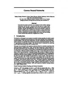
Figure 1: Conditional gradient algorithm for minimizing a smooth function J on F1δ = {f ∈ F1 , γ1 (f ) 6 δ}: going from ft to ft+1 ; see text for details. Conditional gradient algorithm. We assume the function J is convex and L-smooth, that is for all h ∈ L2 (dρ), there exists a gradient J ′ (h) ∈ L2 (dρ) such that for all f ∈ L2 (dρ), 0 6 J(f ) − J(h) − hf − h, J ′ (h)iL2 (dρ) 6

L kf − hk2L2 (dρ) . 2

When X is finite, this corresponds to the regular notion of smoothness from convex optimization (Nesterov, 2004). The conditional gradient algorithm is an iterative algorithm, starting from any point f0 ∈ F1δ and with the following recursion, for t > 0: f¯t

∈ arg min hf, J ′ (ft )iL2 (dρ) f ∈F1δ

ft+1 = (1 − ρt )ft + ρt f¯t . 2 See an illustration in Figure 1. We may choose either ρt = t+1 or perform a line search for ρt ∈ [0, 1]. For all of these strategies, the t-th iterate is a convex combination of the functions f¯0 , . . . , f¯t−1 , and is thus an element of F1δ . It is known that for these two strategies for ρt , we have the following convergence rate:

J(ft ) − inf 6 f ∈F1δ

2L sup kf − gk2L2 (dρ) . t + 1 f,g∈F δ 1

When, r 2 = supv∈V kϕv k2L2 (dρ) is finite, we have kf k2L2 (dρ) 6 r 2 γ1 (f )2 and thus we get a conver-

gence rate of

2Lr 2 δ2 t+1 .

Moreover, the basic FW algorithm may be extended to handle the regularized problem as well (Harchaoui et al., 2013; Bach, 2013; Zhang et al., 2012), with similar convergence rates in O(1/t). Also, the second step in the algorithm, may be replaced by the optimization of J over the convex hull of all functions f¯0 , . . . , f¯t , a variant which is often referred to as fully corrective. In our context where V is a space where local search techniques may be considered, there is also the possibility of fine-tuning the vectors v as well (Bengio et al., 2006). 7

BACH

Adding a new basis function. The conditional gradient algorithm presented above relies on solving at each iteration the “Frank-Wolfe step”: max hf, giL2 (dρ) .

γ(f )6δ

′ for R g = −J (ft ) ∈ L2 (dρ). For the norm γ1 defined through an L1 -norm, we have for f = V ϕv dµ(v) such that γ1 (f ) = |µ|(V):

Z

Z Z

ϕv (x)dµ(v) g(x)dρ(x)

f (x)g(x)dρ(x) = X V Z Z ϕv (x)g(x)dρ(x) dµ(v) = V X Z ϕv (x)g(x)dρ(x) , 6 γ1 (f ) · max v∈V

hf, giL2 (dρ) =

X

X

with equality if and only if µ = µ+ − µ− with µ+R and µ− two non-negative measures, with µ+ (resp. µ− ) supported in the set of maximizers v of | X ϕv (x)g(x)dρ(x)| where the value is positive (resp. negative). This implies that: max hf, giL2 (dρ)

γ1 (f )6δ

Z = δ max ϕv (x)g(x)dρ(x) , v∈V

(1)

X

with the maximizers f of the first problem obtained as δ times convex combinations of ϕv and −ϕv for maximizers v of the second problem. Finitely many observations. When X is finite (or when using the result from Section 2.2), the Frank-Wolfe step in Eq. (1) becomes equivalent to for some vector g ∈ Rn : n n 1 X 1X sup gi f (xi ) = δ max gi ϕv (xi ) , v∈V n γ1 (f )6δ n i=1

(2)

i=1

where the set of solutions of the first problem is the convex hull of the solutions of the second problem. Non-smooth loss functions. In this paper, in our theoretical results, we consider non-smooth loss functions for which conditional gradient algorithms do not converge in general. One possibility is to smooth the loss function, as done by Nesterov (2005): an approximation √ error of ε may be obtained with a smoothness constant proportional to 1/ε. By choosing ε as 1/ t, we obtain a convergence √ rate of O(1/ t) after t iterations. See also Lan (2013). Approximate oracles. The conditional gradient algorithm may deal with approximate oracles; however, what we need in this paper is not the additive errors situations considered by Jaggi (2013), but multiplicative ones on the computation of the dual norm (similar to ones derived by Bach (2013) for the regularized problem). 8

B REAKING

THE

C URSE

OF

D IMENSIONALITY

WITH


Indeed, in our context, we minimize a function J(f ) on f ∈ L2 (dρ) over a norm ball {γ1 (f ) 6 δ}. A multiplicative approximate oracle outputs for any g ∈ L2 (dρ), a vector fˆ ∈ L2 (dρ) such that γ1 (fˆ) = 1, and hfˆ, gi 6 max hf, gi 6 κ hfˆ, gi, γ1 (f )61

for a fixed κ > 1. In Appendix B, we propose a modification of the conditional gradient algorithm that converges to a certain h ∈ L2 (dρ) such that γ1 (h) 6 δ and for which inf γ1 (f )6δ J(f ) 6 J(h) 6 inf γ1 (f )6δ/κ J(f ). Such approximate oracles are not available in general, because they require uniform bounds over all possible values of g ∈ L2 (dρ). In Section 5.5, we show that a weaker form of oracle is sufficient to preserve our generalization bounds. Approximation of any function by a finite number of basis functions. The Frank-Wolfe algorithm may be applied in the function space F1 with J(f ) = 21 E[(f (x) − g(x))2 ], we get a function ft , supported by t basis functions such that E[(ft (x) − g(x))2 ] = O(γ(g)2 /t). Hence, any function in F1 may be approximated with averaged error ε with t = O([γ(g)/ε]2 ) units. Note that the conditional gradient algorithm is one among many ways to obtain such approximation with ε−2 units (Barron, 1993; Kurkova and Sanguineti, 2001). See Section 4.1 for a (slightly) better dependence on ε for convex neural networks.

3. Neural networks with non-decreasing positively homogeneous activation functions In this paper, we focus on a specific family of basis functions, that is, of the form x 7→ σ(w⊤ x + b), for specific activation functions σ. We assume that σ is non-decreasing and positively homogeneous of some integer degree, i.e., it is equal to σ(u) = (u)α+ , for α ∈ {0, 1, . . .}. We focus on these functions for several reasons: – Since they are not polynomials, they may approach any measurable function (Leshno et al., 1993). – By homogeneity, they are invariant by a change of scale of the data; indeed, if all observations x are multiplied by a constant, we may simply change the measure µ defining the expansion of f by the appropriate constant to obtain exactly the same function. This allows us to study functions defined on the unit-sphere. – The special case α = 1, often referred to as the rectified linear unit, has seen considerable recent empirical success (Nair and Hinton, 2010; Krizhevsky et al., 2012), while the case α = 0 (hard thresholds) has some historical importance (Rosenblatt, 1958). Boundedness assumptions. For the theoretical analysis, we assume that our data inputs x ∈ Rd are almost surely bounded by R in ℓq -norm, for q ∈ [2, ∞] (typically q = 2 and q = ∞). We then build the augmented variable z ∈ Rd+1 as z = (x⊤ , R)⊤ ∈ Rd+1 by appending the constant R to 9

BACH

√ x ∈ Rd . We therefore have kzkq 6 2R. By defining the vector v = (w⊤ , b/R)⊤ ∈ Rd+1 , we have: ϕv (x) = σ(w⊤ x + b) = σ(v ⊤ z) = (v ⊤ z)α+ , which now becomes a function of z ∈ Rd+1 . Without loss of generality (and by homogeneity of σ), we may assume that the ℓp -norm of each vector v is equal to 1/R, that is V will be the (1/R)-sphere for the ℓp -norm, where 1/p + 1/q = 1 (and thus p ∈ [1, 2], with corresponding typical values p = 2 and p = 1). This implies that ϕv (x)2 6 2α . Moreover this leads to functions in F1 that are bounded everywhere, that is, ∀f ∈ F1 , f (x)2 6 2α γ1 (f )2 . Note that the functions in F1 are also Lipschitz-continuous for α > 1. Noth that this normalization ensures that γ1 (f ) is homogeneous to the values that f takes, that is, it has the same units. √ Since all ℓp -norms (for p ∈ [1, 2]) are equivalent to each other with constants of at most d with respect to the ℓ2 -norm, all the spaces F1 defined above are equal, but the norms γ1 are of course different and they differ by a constant of at most dα/2 —this can be seen by computing the dual norms like in Eq. (2) or Eq. (1).

Homogeneous reformulation. In our study of approximation properties, it will be useful to consider the the spaceR of function G1 defined for z in the unit sphere Sd ⊂ Rd+1 of the Euclidean norm, such that g(z) = Sd σ(v ⊤ z)dµ(v), with the norm γ1 (g) defined as the infimum of |µ|(Sd ) over all decompositions of g. Note the slight overloading of notations for γ1 (for norms in G1 and F1 ) which should not cause any confusion. In order to prove the approximation properties (with unspecified constants depending only on d), we may assume that p = 2, since the norms k · kp for p ∈ [1, ∞] are equivalent to k · k2 with a constant that grows at most as dα/2 with respect to the ℓ2 -norm. We thus focus on the ℓ2 -norm in all proofs in Section 4. We may go from G1 (a space of real-valued functions defined on the unit ℓ2 -sphere in d + 1 dimensions) to the space F1 (a space of real-valued functions defined on the ball of radius R for the ℓ2 -norm) as follows: α/2 2 1 x kxk g p – Given g ∈ G1 , we define f ∈ F1 , with f (x) = R22 + 1 . If 2 2 R kxk + R 2 R g may be represented as Sd σ(v ⊤ z)dµ(v), then the function f that we have defined may be represented as α kxk2 α/2 Z x 1 2 ⊤ dµ(v) f (x) = +1 v p 2 2 2 R kxk2 + R R + Sd α Z Z ⊤ x/R = σ(w⊤ x + b)dµ(Rw, b), v dµ(v) = 1 d d S S + that is γ1 (f ) 6 γ1 (g), because we have assumed that (w⊤ , b/R)⊤ is on the (1/R)-sphere. α – Conversely, given f ∈ F1 , for z = (t⊤ , a)⊤ ∈ Sd , we define g(z) = g(t, a) = f ( Rt a )a , 1 ⊤ ⊤ d which we define as such on the set of z = (t , a) ∈ R ×R (of unit norm) such that a > √2 .

10

B REAKING

THE

C URSE

OF

D IMENSIONALITY

WITH


p √ Since we always assume kxk2 6 R, we have kxk22 + R2 6 2R, and the value of g(z, a) for a > √12 is enough to recover f from the formula above. √ On that portion {a > 1/ 2} of the sphere Sd , this function exactly inherits the differentiability properties of f . That is, (a) if f is bounded by 1 and f is (1/R)-Lipschitz-continuous, then g is Lipschitz-continuous with a constant that only depends on d and α and (b), if all derivatives of order less than k are bounded by R−k , then all derivatives of the same order of g are bounded by a constant that only depends on d and α. Precise notions of differentiability may be defined on the sphere, using the manifold structure (see, e.g., Absil et al., 2009) or through polar coordinates (see, e.g., Atkinson and Han, 2012, Chapter 3). See these references for more details. The only remaining important aspect is to define g on the entire sphere, so that (a) its regularity constants are controlled by a constant times the ones on the portion of the sphere where it is already defined, (b) g is either even or odd (this will be important in Section 4). Ensuring that the regularity conditions can be met is classical when extending to the full sphere (see, e.g., Whitney, 1934). Ensuring that the function may be chosen as odd or even may be obtained by multiplying the function g by an infinitely differentiable function which is equal to one for √ a > 1/ 2 and zero for a 6 0, and extending by −g or g on the hemi-sphere a < 0. In summary, we may consider in Section 4 functions defined on the sphere, which are much easier to analyze. In the rest of the section, we specialize some of the general concepts reviewed in Section 2 to our neural network setting with specific activation functions, namely, in terms of corresponding kernel functions and geometric reformulations of the Frank-Wolfe steps. 3.1 Corresponding positive-definite kernels In this section, we consider the ℓ2 -norm on the input weight vectors w (that is p = 2). We may compute for x, x′ ∈ Rd the kernels defined in Section 2.3: kα (x, x′ ) = E[(w⊤ x + b)α+ (w⊤ x′ + b)α+ ], d , and x, x′ ∈ Rd+1 . Given the angle for (Rw, b) distributed uniformly on the unit ℓr 2 -sphere S r kxk22 kx′ k22 x⊤ x′ ϕ ∈ [0, π] defined through + 1 = cos ϕ + 1 + 1, we have explicit expresR2 R2 R2 sions (Le Roux and Bengio, 2007; Cho and Saul, 2009):

k0 (z, z ′ ) = ′

k1 (z, z ) = k2 (z, z ′ ) =

1 (π − ϕ) 2π q q kxk22 R2

+1

kx′ k22 R2

+1

((π − ϕ) cos ϕ + sin ϕ) 2(d + 1)π 2 ′ 2 kxk2 kx k2 + 1 + 1 2 2 R R (3 sin ϕ cos ϕ + (π − ϕ)(1 + 2 cos2 ϕ)). 2π[(d + 1)2 + 2(d + 1)]

There are key differences and similarities between the RKHS F2 and our space of functions F1 . The RKHS is smaller than F1 (i.e., the norm in the RKHS is larger than the norm in F1 ); this implies 11

BACH

that approximation properties of the RKHS are transferred to F1 . In fact, our proofs rely on this fact. However, the RKHS norm does not lead to any adaptivity, while the function space F1 is (see more details in Section 5). This may come as a paradox: both the RKHS F2 and F1 have similar properties, but one is adaptive while the other one is not. A key intuitive difference is as follows: R R given a function f expressed as f (x) =R V ϕv (x)p(v)dτ (v), then γ1 (f ) = V |p(v)|dτ (v), while the squared RKHS norm is γ2 (f )2 = V |p(v)|2 dτ (v). For the L1 -norm, the measure p(v)dτ (v) may tend to a singular distribution with a bounded norm, while this is not true for the L2 -norm. For example, the function (w⊤ x + b)α+ is in F1 , while it is not in F2 in general. 3.2 Incremental optimization problem for α = 0 We consider the problem in Eq. (2) for the special case α = 0. For z1 , . . . , zn ∈ Rd+1 and a vector y ∈ Rn , the goal is to solve (as well as the corresponding problem with y replaced by −y):

max

v∈Rd+1

n X i=1

yi 1v⊤ zi >0 = max

v∈Rd+1

X

i∈I+

|yi |1v⊤ zi >0 −

X

i∈I−

|yi |1v⊤ zi >0 ,

where I+ = {i, yi > 0} and I− = {i, yi < 0}. As outlined by Bengio et al. (2006), this is equivalent to finding an hyperplane parameterized by v that minimizes a weighted mis-classification rate (when doing linear classification). Note that the norm of v has no effect.

NP-hardness. This Pn problem is NP-hard in general. Indeed, if we assume that all yi are equal to −1 or 1 and with i=1 yi = 0, Pthen we have a balanced binary classification problem (we need to assume n even). The quantity ni=1 yi 1v⊤ zi >0 is then n2 (1 − 2e) where e is the corresponding classification error for a problem of classifying at positive (resp. negative) the examples in I+ (resp. I− ) by thresholding the linear classifier v ⊤ z. Guruswami and Raghavendra (2009) showed that for all (ε, δ), it is NP-hard to distinguish between instances (i.e., configurations of points xi ), where a halfspace with classification error at most ε exists, and instances where all half-spaces have an error of at leastP 1/2−δ. Thus, it is NP-hard to distinguish between instances where there v ∈ Rd+1 such Pexists n n n d+1 v ∈ R , i=1 yi 1v⊤ zi >0 6 nδ. that i=1 yi 1v⊤ zi >0 > 2 (1 − 2ε) and instances where for all P Thus, it is NP-hard to distinguish instances where maxv∈Rd+1 ni=1 yi 1v⊤ zi >0 > n2 (1 − 2ε) and ones where it is less than n2 δ. Since this is valid for all δ and ε, this rules out a constant-factor approximation.

Convex relaxation. Given linear binary classification problems, there are several algorithms to approximately find a good half-space. These are based on using convex surrogates (such as the hinge loss or the logistic loss). Although some theoretical results do exist regarding the classification performance of estimators obtained from convex surrogates (Bartlett et al., 2006), they do not apply in the context of linear classification. 12

B REAKING

THE

C URSE

OF

D IMENSIONALITY

WITH


3.3 Incremental optimization problem for α = 1 We consider the problem in Eq. (2) for the special case α = 1. For z1 , . . . , zn ∈ Rd+1 and a vector y ∈ Rn , the goal is to solve (as well as the corresponding problem with y replaced by −y): max

kvkp 61

n X

yi (v ⊤ zi )+ = max

kvkp 61

i=1

X

i∈I+

(v ⊤ |yi |zi )+ −

X

i∈I−

(v ⊤ |yi |zi )+ ,

where I+ = {i, yi > 0} and I− = {i, yi < 0}. We have, with ti = |yi |zi ∈ Rd+1 , using convex duality: max

kvkp 61

n X

yi (v ⊤ zi )+ =

max

kvkp 61

i=1

=

max

kvkp 61

=

X

i∈I+

X

i∈I+

(v ⊤ ti )+ − max

bi ∈[0,1]

max

max

max

min

X

i∈I−

bi vi⊤ ti

b∈[0,1]I+

=

max

−

X

i∈I−

max bi v ⊤ ti

bi ∈[0,1]

min v [T+⊤ b+ − T−⊤ b− ]

b∈[0,1]I+ kvkp 61 b∈[0,1]I−

=

(v ⊤ ti )+

b∈[0,1]I−

⊤

max v ⊤ [T+⊤ b+ − T−⊤ b− ] by Fenchel duality,

kvkp 61

min

b+ ∈[0,1]I+ b− ∈[0,1]I−

kT+⊤ b+ − T−⊤ b− kq ,

where T+ ∈ Rn+ ×d has rows ti , i ∈ I+ and T− ∈ Rn− ×d has rows ti , i ∈ I− , with v ∈ arg maxkvkp 61 v ⊤ (T+⊤ b+ − T−⊤ b− ). The problem thus becomes max

min

b+ ∈[0,1]n+ b− ∈[0,1]n−

kT+⊤ b+ − T−⊤ b− kq .

P For the problem of maximizing | ni=1 yi (v ⊤ zi )+ |, then this corresponds to ⊤ ⊤ ⊤ ⊤ max maxn min n kT+ b+ − T− b− kq , maxn min n kT+ b+ − T− b− kq . b+ ∈[0,1]

+

b− ∈[0,1]

b− ∈[0,1]

−

−

b+ ∈[0,1]

+

This is exactly the Hausdorff distance between the two convex sets {T+⊤ b+ , b+ ∈ [0, 1]n+ } and {T−⊤ b− , b− ∈ [0, 1]n− } (referred to as zonotopes, see below). Given the pair (b+ , b− ) achieving the Hausdorff distance, then we may compute the optimal v as v = arg maxkvkp 61 v ⊤ (T+⊤ b+ − T−⊤ b− ). Note this has not changed the problem at all, since it is equivalent. It is still NP-hard in general (König, 2014). But we now have a geometric interpretation with potential approximation algorithms. See below and Section 6. Zonotopes. A zonotope A is the Minkowski sum of a finite number of segments from the origin, that is, of the form A = [0, t1 ] + · · · + [0, tr ] = 13

r nX i=1

o bi ti , b ∈ [0, 1]r ,

BACH

t1 + t2 + t3

t1 t3 t2 0

0

0

0

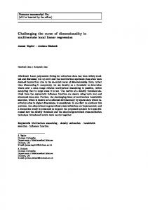
Figure 2: Two zonotopes in two dimensions: (left) vectors, and (right) their Minkowski sum (represented as a polygone).

0

0 0

0

Figure 3: Left: two zonotopes (with their generating segments) and the segments achieving the two sides of the Haussdorf distance. Right: approximation by ellipsoids.

for some vectors ti , i = 1, . . . , r (Bolker, 1969). See an illustration in Figure 2. They appear in several areas of computer science (Edelsbrunner, 1987; Guibas et al., 2003) and mathematics (Bolker, 1969; Bourgain et al., 1989). In machine learning, they appear naturally as the affine projection of a hypercube; in particular, when using a higher-dimensional distributed representation of points in Rd with elements in [0, 1]r , where r is larger than d (see, e.g., Hinton and Ghahramani, 1997), the underlying polytope that is modelled in Rd happens to be a zonotope. In our context, the two convex sets {T+⊤ b+ , b+ ∈ [0, 1]n+ } and {T−⊤ b− , b− ∈ [0, 1]n− } defined above are thus zonotopes. See an illustration of the Hausdorff distance computation in Figure 3 (middle plot), which is the core computational problem for α = 1. Approximation by ellipsoids. Centrally symmetric convex polytopes (w.l.o.g. centered around zero) may be approximated by ellipsoids. In our set-up, we could use the minimum volume enclosing ellipsoid (see, e.g. Barvinok, 2002), which can be computed exactly when the polytope is given through its vertices, or up to a constant factor when the polytope is such that quadratic functions may be optimized with a constant factor approximation. For zonotopes, the standard semi-definite relaxation of Nesterov (1998) leads to such constant-factor approximations, and thus the minimum volume inscribed ellipsoid √ may be computed up to a constant. Given standard results (see, e.g. Barvinok, 2002), a (1/ d)-scaled version of the ellipsoid is inscribed in this polytope, √ and thus the ellipsoid is a provably good approximation of the zonotope with a factor scaling as d. However, the approximation ratio is not good enough to get any relevant bound for our purpose (see Sec14

B REAKING

THE

C URSE

OF

D IMENSIONALITY

WITH


tion 5.5), as for computing the Haussdorff distance, we care about potentially vanishing differences that are swamped by constant factor approximations. Nevertheless, the ellipsoid approximation may prove useful in practice, in particular because the ℓ2 Haussdorff distance between two ellipsoids may be computed in polynomial time (see Appendix E). 3.4 Incremental optimization problem for α > 2 We consider the problem in Eq. (2) for the remaining cases α > 2. For z1 , . . . , zn ∈ Rd+1 and a vector y ∈ Rn , the goal is to solve (as well as the corresponding problem with y replaced by −y): n X 1 X 1 1X yi (v ⊤ zi )α+ = max (v ⊤ |yi |1/α zi )α+ − (v ⊤ |yi |1/α zi )α+ , α α kvkp 61 kvkp 61 α

max

i=1

i∈I+

i∈I−

where I+ = {i, yi > 0} and I− = {i, yi < 0}. We have, with ti = |yi |1/α zi ∈ Rd+1 , and β ∈ (1, 2] defined by 1/β + 1/α = 1 (we use the fact that the function u → 7 uα /α and v 7→ v β /β are Fenchel-dual to each other): n

1X max yi (v ⊤ zi )α+ = α kvkp 61 i=1

X 1 X 1 (v ⊤ ti )α+ − (v ⊤ ti )α+ α α kvkp 61 i∈I+ i∈I− n n X 1 o 1 o X max bi v ⊤ ti − bβi max bi vi⊤ ti − bβi − = max bi >0 bi >0 β β kvkp 61 max

i∈I−

i∈I+

=

max min max v ⊤ [T+⊤ b+ − T−⊤ b− ] −

I b∈R++

I b∈R+−

kvkp 61

1 1 kb+ kββ + kb− kββ β β

by Fenchel duality, 1 1 = max min kT+⊤ b+ − T−⊤ b− kq − kb+ kββ + kb− kββ , (3) I+ I− β β b+ ∈[0,1] b− ∈[0,1] where T+ ∈ Rn+ ×d has rows ti , i ∈ I+ and T− ∈ Rn− ×d has rows ti , i ∈ I− , with v ∈ arg maxkvkp 61 (T+⊤ b+ − T−⊤ b− )⊤ v. Contrary to the case α = 1, we do not obtain exactly a formulation as a Hausdorff distance. However, if we consider the convex sets Kλ+ = {T+⊤ b+ , b+ > 0, kb+ kβ 6 λ} and Kµ− = {T−⊤ b− , b− > 0, kb− kβ 6 µ}, then, a solution of Eq. (3) may be obtained from Hausdorff distance computations between Kλ+ and Kµ− , for certain λ and µ.

4. Approximation properties In this section, we consider the approximation properties of the set F1 of functions defined on Rd . As mentioned earlier, the norm used to penalize input weights w or v is irrelevant for approximation properties as all norms are equivalent. Therefore, we focus on the case q = p = 2 and ℓ2 -norm constraints. Because we consider homogeneous activation functions, we start by studying the set G1 of functions defined on the unit ℓ2 -sphere Sd ⊂ Rd+1 . We denote by τd the uniform probability measure on Sd . 15

BACH

R ⊤ The set G1 is defined as the set of functions on the sphere such R that g(z) = Sd σ(v z)p(z)dτd (z), also define with the norm γ1 (g) equal to the smallest possible value of Sd |p(z)|dτd (z). R We may 2 the corresponding squared RKHS norm by the smallest possible value of Sd |p(z)| dτd (z), with the corresponding RKHS G2 . In this section, we first consider approximation properties of functions in G1 by a finite number of neurons (only for α = 1). We then study approximation properties of functions on the sphere by functions in G1 . It turns out that all our results are based on the approximation properties of the corresponding RKHS G2 : we give sufficient conditions for being in G2 , and then approximation bounds for functions which are not in G2 . Finally we transfer these to the spaces F1 and F2 , and consider in particular functions which only depend on projections on a low-dimensional subspace, for which the properties of G1 and G2 (and of F1 and F2 ) differ. Approximation properties of neural networks with finitely many neurons have been studied extensively (see, e.g., Petrushev, 1998; Pinkus, 1999; Makovoz, 1998; Burger and Neubauer, 2001). In Section 4.7, we relate our new results to existing work from the literature on approximation theory, by showing that our results provide an explicit control of the various weight vectors which are needed for bounding the estimation error in Section 5. 4.1 Approximation by a finite number of basis functions A key quantity that drives the approximability by a finite number of neurons is the variation norm γ1 (g). As shown in Section 2.5, any function g such that γ1 (g) is finite, may be approximated in L2 (Sd )-norm with error ε with n = O(γ1 (g)2 ε−2 ) units. For α = 1 (rectified linear units), we may improve the dependence in ε, through the link with zonoids and zonotopes, as we now present. If we decompose the signed measure R µ as µ = µ+ − µR− where µ+ and µ− are positive measures, then, for g ∈ G1 , we have g(z) = Sd (v ⊤ z)+ dµ+ (v) − Sd (v ⊤ z)+ dµ− (v) = g+ (z) − g− (z), which is a decomposition of g as a difference of positively homogenous convex functions. Positively homogenous convex functions h may be written as the support function of a compact convex set K (Rockafellar, 1997), that is, h(z) = maxy∈K y ⊤ z, and the set K characterizes the function h. The functions g+ and g− defined above are not any convex positively homogeneous functions, as we now describe. Pr If the measure µ+ is supported by finitely many points, that is, µ (v) = + i=1 ηi δ(v − vi ) with Pt Pt Pt ⊤ ⊤ ⊤ η > 0, then g+ (z) = i=1 ηi (vi z)+ = i=1 (ηi vi z)+ = i=1P (ti z)+ for ti = ηi vi . Thus the corresponding set K+ is the zonotope [0, t1 ] + · · · + [0, tr ] = { ri=1 bi ti , b ∈ [0, 1]r } already defined in Section 3.3. Thus the functions g+ ∈ G1 and g− ∈ G1 for finitely supported measures µ are support functions of zonotopes. When the measure µ is not constrained to have finite support, then the sets K+ and K− are limits of zonotopes, and thus, by definition, zonoids (Bolker, 1969), and thus functions in G1 are differences of support functions of zonoids. Zonoids are a well-studied set of convex bodies. They are centrally symmetric, and in two dimensions, all centrally symmetric compact convexs sets are (up to translation) zonoids, which is not true in higher dimensions (Bolker, 1969). Moreover, the problem of approximating a zonoid by a zonotope with a small number of segments (Bourgain et al., 1989;

16

B REAKING

THE

C URSE

OF

D IMENSIONALITY

WITH


Matouˇsek, 1996) is essentially equivalent to the approximation of a function g by finitely many neurons. The number of neurons directly depends on the norm γ1 , as we now show. Proposition 1 (Number of units - α = 1) Let ε ∈ (0, 1/2). For any g function R in G1 , there exists a measure µ supported on at most r points in V, so that for all z ∈ Sd . |g(z) − Sd (v ⊤ z)+ dµ(v)| 6 εγ(g), with r 6 C(d)ε−2d/(d+3) , for some constant C(d) that depends only on d. Proof Without loss of generality, we assume γ(g) = 1. It is shown by Matouˇsek (1996) that for any probability measure µ (positive and with finite mass) on the sphere Sd , there exists a set of r points v1 , . . . , vr , so that for all z ∈ Sd , r 1 X ⊤ |vi z| 6 ε, |v z|dµ(v) − r Sd

Z

⊤

(4)

i=1

with r 6 C(d)ε−2+6/(d+3) = C(d)ε−2d/(d+3) , for some constant C(d) that depends only on d. We may then simply write 1 g(z) = (v z)+ dµ(v) = 2 d S Z

⊤

µ+ (Sd ) (v z)dµ(v)+ 2 Sd

Z

⊤

Z

dµ+ (v) µ− (Sd ) |v z| − µ+ (Sd ) 2 Sd ⊤

Z

Sd

|v ⊤ z|

dµ− (v) , µ− (Sd )

and approximate the last two terms with error εµ± (Sd ) with r terms, leading to an approximation of εµ+ (Sd ) + εµ− (Sd ) = εγ1 (g) = ε, with a remainder that is a linear function q ⊤ z of z, with kqk2 6 1. We may then simply add two extra units with vectors q/kqk2 and weights −kqk2 and kqk2 . We thus obtain, with 2r + 2 units, the desired approximation result. Note that Bourgain et al. (1989, Theorem 6.5) showed that the scaling in ε in Eq. (4) is not improvable, if the measure is allowed to have non equal weights on all points and the proof relies on the non-approximability of the Euclidean ball by centered zonotopes. This results does not apply here, because we may have different weights µ− (Sd ) and µ+ (Sd ). Note that the proposition above is slightly improved in terms of the scaling in ε. The simple use of conditional gradient leads to r 6 ε−2 γ(g)2 , with a better constant (independent of d) but a worse scaling in ε—also with a result in L2 (Sd )-norm and not uniformly on the ball {kxkq 6 R}. Note also that the conditional gradient algorithm gives a constructive way of building the measure. Moreover, the proposition above is related to the result from Makovoz (1998, Theorem 2), which applies for α = 0 but with a number of neurons growing as ε−2d/(d+1) , or to the one of Burger and Neubauer (2001, Example 3.1), which applies to a piecewise affine sigmoidal function but with a number of neurons growing as ε−2(d+1)/(d+3) (both slightly worse than ours). 4.2 Sufficient conditions for finite variation In this section and the next one, we study more R precisely the RKHS G2 (and thus obtain similar results for G1 ⊃ G2 ). The kernel k(x, y) = Sd (v ⊤ x)+ (v ⊤ y)+ dτd (v) defined on the sphere Sd belongs to the family of dot-product kernels (Smola et al., 2001) that only depends on the dotproduct x⊤ y, although in our situation, the function is not particularly simple (see formulas in 17

BACH

Section 3.1). The analysis of these kernels is similar to one of translation-invariant kernels; for d = 1, i.e., on the 2-dimensional sphere, it is done through Fourier series; while for d > 1, spherical harmonics have to be used as the expansion of functions in series of spherical harmonics make the computation of the RKHS norm explicit (see a review of spherical harmonics in Appendix D.1 with several references therein). Since the calculus is tedious, all proofs are put in appendices, and we only present here the main results. In this section, we provide simple sufficient conditions for belonging to G2 (and hence G1 ) based on the existence and boundedness of derivatives, while in the next section, we show how any Lipschitz-function may be approximated by functions in G2 (and hence G1 ) with precise control of the norm of the approximating functions. The derivatives of functions defined on Sd may be defined in several ways, using the manifold structure (see, e.g., Absil et al., 2009) or through polar coordinates (see, e.g., Atkinson and Han, 2012, Chapter 3). For d = 1, the two-dimensional sphere S 1 may be parameterized by a single angle and thus the notion of derivatives and the proof of the following result is simpler and based on Fourier series (see Appendix C.2). For the general proof based on spherical harmonics, see Appendix D.2.

Proposition 2 (Finite variation on the sphere) Assume that g : Sd → R is such that all i-th order derivatives exist and are upper-bounded by η for i ∈ {0, . . . , s}, where s is an integer such that s > (d − 1)/2 + α + 1. Assume g is even if α is odd (and vice-versa); then g ∈ G2 and γ2 (g) 6 C(d, α)η, for a constant C(d, α) that depends only on d and α. We can make the following observations: – Tightness of conditions: as shown in Appendix D.5, there are functions g, which have bounded first s derivatives and do not belong to G2 while s 6 d2 + α (at least when s − α is even). Therefore, the affine scaling in d2 + α is not improvable (but the constant may be). – Dependence on α: for any d, the higher the α, the stricter the sufficient condition. Given that the estimation error grows slowly with α (see Section 5.1), low values of α would be preferred in practice. – Dependence on d: a key feature of the sufficient condition is the dependence on d, that is, as d increases the number of derivatives has to increase linearly in d/2. This is another instantiation of the curse of dimensionality: only very smooth functions in high dimensions are allowed. – Special case d = 1, α = 0: differentiable functions on the sphere in R2 , with bounded derivatives, belong to G2 , and thus all Lipschitz-continuous functions, because Lipschitz-continuous functions are almost everywhere differentiable with bounded derivative (Adams and Fournier, 2003). 4.3 Approximation of Lipschitz-continuous functions In order to derive generalization bounds for target functions which are not sufficiently differentiable (and may not be in G2 or G1 ), we need to approximate any Lipschitz-continuous function, with a function g ∈ G2 with a norm γ2 (g) that will grow as the approximation gets tighter. We give 18

B REAKING

THE

C URSE

OF

D IMENSIONALITY

WITH


precise rates in the proposition below. Note the requirement for parity of the function g. The result below notably shows the density of G1 in uniform norm in the space of Lipschitz-continuous functions of the given parity, which is already known since our activation functions are not polynomials (Leshno et al., 1993). Proposition 3 (Approximation of Lipschitz-continuous functions on the sphere) For δ greater than a constant depending only on d and α, for any function g : Sd → R such that for all x, y ∈ Sd , g(x) 6 η and |g(x) − g(y)| 6 ηkx − yk2 , and g is even if α is odd (and vice-versa), then there exists h ∈ G2 , such that γ2 (h) 6 δ and δ δ −1/(α+(d−1)/2) . log sup |h(x) − g(x)| 6 C(d, α)η η η x∈Sd This proposition is shown in Appendix C.3 for d = 1 (using Fourier series) and in Appendix D.4 for all d > 1 (using spherical harmonics). We can make the following observations: – Dependence in δ and η: as expected, the main term in the error bound (δ/η)−1/(α+(d−1)/2) is a decreasing function of δ/η, that is when the norm γ2 (h) is allowed to grow, the approximation gets tighter, and when the Lipschitz constant of g increases, the approximation is less tight. – Dependence on d and α: the rate of approximation is increasing in d and α. In particular the approximation properties are better for low α. – Special case d = 1 and α = 0: up to the logarithmic term we recover the result of Prop. 2, that is, the function g is in G2 . – Tightness: in Appendix D.5, we provide a function which is not in the RKHS and for which the tightest possible approximation scales as δ−2/(d/2+α−2) . Thus the linear scaling of the rate as d/2 + α is not improvable (but constants are). 4.4 Linear functions In this section, we consider a linear function on Sd , that is g(x) = v ⊤ x for a certain v ∈ Sd , and compute its norm (or upper-bound thereof) both for G1 and G2 , which is independent of v and finite. In the following propositions, the notation ≈ means asymptotic equivalents when d → ∞. Proposition 4 (Norms of linear functions on the sphere) Assume that g : Sd → R is such g(x) = 2dπ ≈ 2π. If α = 1, then γ1 (g) 6 2, v ⊤ x for a certain v ∈ Sd . If α = 0, then γ1 (g) 6 γ2 (g) = d−1 and for all α > 1, γ1 (g) 6 γ2 (g) =

d 4π Γ(α/2+d/2+1) d−1 α Γ(α/2)Γ(d/2+1)

≈ Cdα/2 .

We see that for α√= 1, the γ1 -norm is less than a constant, and is much smaller than the γ2 -norm (which scales as d). For α > 2, we were not able to derive better bounds for γ1 (other than the value of γ2 ). 4.5 Functions of projections If g(x) = ϕ(w⊤ x) for some unit-norm w ∈ Rd+1 and ϕ a function defined on the real-line, then the value of the norms γ2 and γ1 differ significantly. Indeed, for γ1 , we may consider a new variable 19

BACH

x ˜ ∈ S1 ⊂ R2 , with x ˜1 = w⊤ x, and the function g˜(x) = ϕ(˜ x1 ). We may then apply Prop. 2 to g˜ with d = 1. That is, if ϕ is (α + 1)-times differentiable with bounded derivatives, there exists R ⊤ ˜(˜ v )σ(˜ v x ˜)d˜ µ, with γ1 (˜ g ) = |˜ µ|(S1 ). If we consider any vector a decomposition g˜(˜ x) = S 1 µ d+1 d+1 t ∈ R which is orthogonal to w in R , then, we may define a measure µ supported in the circle defined by the two vectors w and t and which is equal to µ ˜ on that circle. The total variation of µ is the one of µ ˜ while g can be decomposed using µ and thus γ1 (g) 6 γ1 (˜ g ). Similarly, Prop. 3 could also be applied (and will for obtaining generalization bounds), also our reasoning works for any low-dimensional projections: the dependence on a lower-dimensional projection allows to reduce smoothness requirements. However, for the RKHS norm γ2 , this reasoning does not apply. For example, a certain function ϕ exists, which is s-times differentiable, as shown in Appendix D.5, for s 6 d2 + α (when s − α is even), and is not in G2 . Thus, given Prop. 2, the dependence on a uni-dimensional projection does not make a difference regarding the level of smoothness which is required to belong to G2 . 4.6 From the unit-sphere Sd to Rd+1 We now extend the results above to functions defined on Rd , to be approximated by functions in F1 and F2 . More precisely, we first extend Prop. 2 and Prop. 3, and then consider norms of linear functions and functions of projections. Proposition 5 (Finite variation) Assume that f : Rd → R is such that all i-th order derivatives exist and are upper-bounded on the ball {kxkq 6 R} by η/Ri for i ∈ {0, . . . , k}, where s is the smallest integer such that s > (d−1)/2+α+1; then f ∈ F2 and γ2 (f ) 6 C(d, α)η, for a constant C(d, α) that depends only on d and α. Proof By assumption, the function x 7→ f (Rx) has all its derivatives bounded by a constant times η. α Moreover, we have defined g(t, a) = f ( Rt a )a so that all derivatives are bounded by η. The result then follows immediately from Prop. 2.

Proposition 6 (Approximation of Lipschitz-continuous functions) For δ larger than a constant that depends only on d and α, for any function f : Rd → R such that for all x, y such that kxkq 6 R and kykq 6 R, |f (x)| 6 η and |f (x) − f (y)| 6 ηR−1 kx − ykq , there exists g ∈ F2 such that γ2 (g) 6 δ and sup |f (x) − g(x)| 6 C(d, α)η

kxkq 6R

δ −1/(α+(d−1)/2) η

log

δ . η

Proof With the same reasoning as above, we obtain that g is Lipschitz-continuous with constant η, we thus get the desired approximation error from Prop. 3.

Linear functions. If f (x) = w⊤ x + b, with kwk2 6 η and b 6 ηR, then for α = 1, it is straightforward that γ1 (f ) 6 2Rη. Moreover, we have γ2 (f ) ∼ CRη. For other values of α, we 20

B REAKING

THE

C URSE

OF

D IMENSIONALITY

WITH


also have γ1 -norms less than a constant (depending only of α) times Rη. The RKHS norms are bit harder to compute since linear functions for f leads to linear functions for g only for α = 1. Functions of projections. If f (x) = ϕ(w⊤ x) where kwk2 6 η and ϕ : R → R is a function, then the norm of f is the same as the norm of the function ϕ on the interval [−Rη, Rη]. This is a consequence of the fact that the total mass of a Radon measure remains bounded even when the support has measure zero (which might not be the case for the RKHS defined in Section 2.3). For the RKHS, there is no such results and it is in general not adaptive. More generally, if f (x) = Φ(W ⊤ x) for W ∈ Rd×s with the largest singular value of W less than η, and Φ a function from Rs to R, then for kxk2 6 R, we have kW ⊤ xk2 6 Rη, and thus we may apply our results for d = s. ℓ1 -penalty on input weights (p=1). When using an ℓ1 -penalty on input weights instead of an ℓ2 penalty, the results in Prop. 5 and 6 are unchanged (only the constants that depend on d are changed). Moreover, when kxk∞ 6 1 almost surely, functions of the form f (x) = ϕ(w⊤ x) where kwk1 6 η and ϕ : R → R is a function, will also inherit from properties of ϕ (without any dependence on dimension). Similarly, for functions of the form f (x) = Φ(W ⊤ x) for W ∈ Rd×s with all columns of ℓ1 -norm less than η, we have kW ⊤ xk∞ 6 Rη and we can apply the s-dimensional result. 4.7 Related work In this section, we show how our results from the previous sections relate to existing work on neural network approximation theory. Approximation of Lipschitz-continuous functions with finitely many neurons. In this section, we only consider the case α = 1, for which we have two approximation bounds: Prop. 6 which approximates any η-Lipschitz-continuous function by a function with finite γ1 -norm less than δ and uniform error less than η(δ/η)−2/(d+1) log (δ/η), and Prop. 1 which shows that a function with γ1 -norm less than δ, may be approximated with r neurons with uniform error δr −(d+3)/(2d) . Thus, given r neurons, we get an approximation of the original function with uniform error η(δ/η)−2/(d+1) log (δ/η) + δr −(d+3)/(2d) . We can optimize over δ, and use δ = ηn(d+1)/(2d) , to obtain a uniform approximation bound proportional to η(log n)n−1/d , for approximating an η-Lipschitz-continuous function with n neurons. Approximation by ridge functions. The approximation properties of single hidden layer neural networks have been studied extensively, where they are often referred to as “ridge function” approximations. As shown by Pinkus (1999, Corollary 6.10)—based on a result from Petrushev (1998), the approximation order of n−1/d for the rectified linear unit was already known, but only in L2 norm (and without the factor log n), and without any constraints on the input and output weights. In this paper, we provide an explicit control of the various weights, which is needed for computing estimation errors. Moreover, while the two proof techniques use spherical harmonics, the proof of Petrushev (1998) relies on quadrature formulas for the associated Legendre polynomials, while 21

BACH

ours relies on the relationship with the associated positive definite kernels, is significantly simpler, and offers additional insights into the problem (relationship with convex neural networks and zonoids). Maiorov (2006, Theorem 2.3) also derives a similar result, but in L2 -norm (rather than uniform norm), and for sigmoidal activation functions (which are bounded). Note finally, that the order O(n−1/d ) cannot be improved (DeVore et al., 1989, Theorem 4.2). Also, Maiorov and Meir (2000, Theorem 5) derive similar upper and lower bounds based on a random sampling argument which is close to using random features in the RKHS setting described in Section 2.3.

5. Generalization bounds Our goal is to derive the generalization bounds outlined in Section 2.4. That is, given some distribution over the pairs (x, y) ∈ X × Y, a loss function ℓ : Y × R → R, our aim is to find a function f : Rd → R such that J(f ) = E[ℓ(y, f (x))] is small, given some i.i.d. observations (xi , yi ), i = 1, . . . , n. We consider the empirical risk minimization framework over a space of functions F, equipped with aP norm γ (in our situations, F1 and F2 , equipped with γ1 or γ2 ). The empirical risk Jˆ(f ) = n1 ni=1 ℓ(yi , f (xi )), is minimized by constraining f to be in the ball F δ = {f ∈ F, γ(f ) 6 δ}. We assume√that almost surely, kxkq 6 R, that the function u 7→ ℓ(y, u) is G-Lipschitz-continuous ⊤ ⊤ on {|u| 6 √ 2δ}, and that almost surely, ℓ(y, 0) 6 Gδ. As before z denotes z = (x , R) so that kzkq 6 2R. This corresponds to the following examples: – Logistic regression and support vector machines: we have G = 1. √ 2 √ ∞ }. – Least-squares regression: we take G = max { 2δ + kyk∞ , kyk 2δ Approximation errors inf f ∈F δ J(f ) − inf f ∈F J(f ) will be obtained from the approximation results from Section 4 by assuming that the optimal target function f∗ has a specific form. Indeed, we have: n o inf J(f ) − J(f∗ ) 6 G inf sup |f (x) − f∗ (x)| . f ∈F δ

f ∈F δ

kxkq 6R

ˆ ) − J(f )| using Rademacher complexities. We now deal with estimation errors supf ∈F δ |J(f 5.1 Estimation errors and Rademacher complexity ˆ The following proposition bounds the uniform deviation between J and its empirical counterpart J. This result is standard (see, e.g., Bartlett and Mendelson, 2003) and may be extended in bounds that hold with high-probability. Proposition 7 (Uniform deviations) We have the following bound on the expected uniform deviation: Gδ ˆ )| 6 4 √ E sup |J(f ) − J(f C(p, d, α), n γ1 (f )6δ with the following constants: 22

B REAKING

THE

C URSE

OF

D IMENSIONALITY

WITH


p – for α > 1, C(p, d, α) 6 α 2 log(d + 1) for p = 1 and C(p, d, α) 6

√α p−1

√ – for α = 0, C(p, d, α) 6 C d + 1, where C is a universal constant.

for p ∈ (1, 2]

Proof We use the standard framework of Rademacher complexities and get: ˆ )| E sup |J(f ) − J(f γ1 (f )6δ

6

6

6

6

n 1 X 2E sup τi ℓ(yi , f (xi )) using Rademacher random variables τi , γ1 (f )6δ n i=1 n n 1 X 1 X τi ℓ(yi , 0) + 2E sup τi [ℓ(yi , f (xi )) − ℓ(yi , 0)] 2E sup γ1 (f )6δ n i=1 γ1 (f )6δ n i=1 X 1 n Gδ 2 √ + 2GE sup τi f (xi ) using the Lipschitz-continuity of the loss, n γ(f )6δ n i=1 n 1 X Gδ ⊤ α τi (v zi )+ using Eq. (2). 2 √ + 2GδE sup n kvkp 61/R n i=1

We then take different routes for α > 1 and α = 0. For α > 1, we have the upper-bound

X 1 n Gδ ⊤ ˆ τi v zi E sup |J(f ) − J(f )| 6 2 √ + 2GδαE sup n kvkp 61/R n γ1 (f )6δ i=1

using the α-Lipschitz-cont. of (·)α+ on [−1, 1],

n

X

Gδ Gαδ

6 2√ + 2 E τi zi

. Rn n q i=1

From Kakade et al. (2009), we get the following bounds on Rademacher complexities: – If p ∈ (1, 2], then q ∈ [2, ∞), and Ek – If p = 1, then q = ∞, and Ek Overall, we have Ek

Pn

i=1 τi zi kq

6

Pn

Pn

i=1 τi zi kq

i=1 τi zi kq

√

6

√ √ q − 1R n =

√1 R p−1

√

n

√ p 6 R n 2 log(d + 1).

nRC(p, d) with C(p, d) defined above, and thus

Gδα Gδ ˆ )| 6 2 √ (1 + αC(p, d)) 6 4 √ C(p, d). E sup |J(f ) − J(f n n γ(f )6δ For α = 0, we can simply go through the VC-dimension of half-hyperplanes, which is equal to d, 1 Pn and Theorem 6 from Bartlett and Mendelson (2003), that shows that E supv∈Rd+1 n i=1 τi 1v⊤ zi 6 C

√ d+1 √ , n

where C is a universal constant.

23

BACH

Note that using standard results from Rademacher complexities, we have, r with probability greater 2 2Gδ ˆ )| + √ than 1 − u, sup |J(f ) − Jˆ(f )| 6 E sup |J(f ) − J(f log . n u γ1 (f )6δ γ1 (f )6δ

5.2 Generalization bounds for ℓ2 -norm constraints on input weights (p = 2) We now provide generalization bounds for the minimizer of the empirical risk given the contraint that γ1 (f ) 6 δ for a well chosen δ, that will depend on the assumptions regarding the target function f∗ , listed in Section 1. In this section, we consider an ℓ2 -norm on input weights w, while in the next section, we consider the ℓ1 -norm. The two situations are summarized and compared in Table 1, where we consider that √ kxk∞ 6 r almost surely, which implies that our bound R will depend on dimension as R 6 r d. Our generalization bounds are expected values of the excess expected risk for a our estimator (where the expectation is taken over the data). Affine functions. We assume f∗ (x) = w⊤ x + b, with kwk2 6 η and |b| 6 Rη. Then, as seen in Section 4.6, f∗ ∈ F1 with γ1 (f∗ ) 6 C(α)ηR. From Prop. 7, we thus get a generalization bound √ times a constant (that may depend on α), which is the same as assuming directly proportional to GRη n that we optimize over linear predictors only. The chosen δ is then a constant times Rη, and does not grow with n, like in parametric estimation (although we do use a non-parametric estimation procedure). P Projection pursuit. We assume f∗ (x) = kj=1 fj (wj⊤ x), with kwj k2 6 η and each fj bounded by ηR and 1-Lipschitz continuous. From Prop. 6, we may approach each x 7→ fj (wj⊤ x) by a function with γ1 -norm less than δηR and uniform approximation C(α)ηRδ−1/α log δ. This leads to a total approximation error of kC(α)GηRδ−1/α log δ for a norm less than kδηR. For α > 1, from Prop. 7, the estimation error is

kGRηδ √ , n

with an overall bound of C(α)kGRη( √δn +

δ−1/α log δ). With δ = nα/2(α+1) (which grows with n), we get an optimized generalization bound log n , with a scaling independent of the dimension d (note however that R typiof C(α)kGRη n1/(2α+2) √ √ cally grow with d, i.e., r d, if we have a bound in ℓ∞ -norm for all our inputs x). For α = 0, from Prop. 5, the target function belongs to F1 with a norm less than kGRη, leading to √ kGRη d an overall generalization bound of √n . Note that when the functions fj are exactly the activation functions, the bound is better, as these functions directly belong to the space F1 . Multi-dimensional projection pursuit. We extend the situation above, by assuming f∗ (x) = P k ⊤ d×s having all singular values less than η and each F bounded j j=1 Fj (Wj x) with each Wj ∈ R by ηR and 1-Lipschitz continuous. From Prop. 6, we may approach each x 7→ Fj (Wj⊤ x) by a function with γ1 -norm less than δηR and uniform approximation C(α, s)ηRδ−1/(α+(s−1)/2) log δ. This leads to a total approximation error of kC(α, s)GηRδ−1/(α+(s−1)/2) log δ. 24

B REAKING

THE

function space ⊤ w x+b

k X fj (wj⊤ x), wj ∈ Rd

C URSE

OF

D IMENSIONALITY

k · k2 , α > 1

kd1/2

log n


k · k1 , α > 1

α=0

√ log d 1/2 q( n )

(dq)1/2 n1/2

kq 1/2 (log d)1/(α+1) log n n1/(2α+2)

k(dq)1/2 n1/2

d1/2 n1/2

1/(2α+2)

WITH

n j=1 X k kq 1/2 (log d)1/(α+(s+1)/2) (dq)1/2 d1/(s+1) kd1/2 fj (Wj⊤ x), Wj ∈ Rd×s log n log n 1/(2α+s+1) log n 1/(2α+s+1) 1/(s+1) n n n j=1 Table 1: Summary of generalization bounds. See text for details.

√ √ For α > 1, the estimation error is kGRηδ/ n, with an overall bound of C(α, s)kGRη(δ/ n + δ−1/(α+(s−1)/2) log δ). With δ = n(α+(s−1)/2)/(2α+s−1) , we get an optimized bound of C(α,s)kGRη log n. n1/(2α+s+1) For α = 0, we have an overall bound of C(s)kGRη(δ−2/(s−1) log δ + (n/d)(s−1)/(s+1) , we get a generalization bound scaling as

C(s)kGRη (n/d)1/(s+1)

√ δ√ d ), n

and with δ =

log(n/d).

Note that for s = d and k = 1, we recover the usual Lipschitz-continuous assumption, with a rate of C(α,d)kGRη log n. n1/(2α+d+1) We can make the following observations: √ – Summary table: when we know a bound r on all dimensions of x, then we may take R = r d; this is helpful in comparisons in Table 1. – Dependence on d: when making only a global Lipschitz-continuity assumption, the generalization bound has a bad scaling in n, i.e., as n−1/(2α+d+1) , which goes down to zero slowly when d increases. However, when making structural assumptions regarding the dependence on unknown lower-dimensional subspaces, the scaling in d disappears. – Comparing different values of α: the value α = 0 always has the best scaling in n, but constants are better for α > 1 (among which α = 1 has the better scaling in n). – Bounds for F2 : The simplest upper bound for the penalization by the space F2 depends √ on the approximation√properties of F2 . For linear functions and α = 1, it is less than dηR, √ d . For the other values of α, there is a constant C(d). Otherwise, there with a bound GRη n is no adaptivity and all other situations only lead to upper-bounds of O(n−1/(2α+d+1) ). See more details in Section 5.4. – Sample complexity: Note that the generalization bounds above may be used to obtain sample complexity results such as dε−2 for affine functions, (εk−1 d−1/2 )−2α−2 for projection pursuit, and (εk−1 d−1/2 )−s−1−2α for the generalized version (up to logarithmic terms). – Relationship to existing work: Maiorov (2006, Theorem 1.1) derives similar results for neural networks with sigmoidal activation functions (that tend to one at infinity) and the square loss 25

BACH

only, and for a level of smoothness of the target function which grows with dimension (in this case, once can get easily rates of n−1/2 ). Our result holds for problems where only bounded first-order derivatives are assumed. Lower bounds. In the sections above, we have only provided generalization bounds. Although interesting, deriving lower-bounds for the generalization performance when the target function belongs to certain function classes is out of the scope of this paper. Note however, that results from Sridharan (2012) suggest that the Rademacher complexities of the associated function classes provide such lower-bounds. For general Lipschitz-functions, these Rademacher complexities decreases as n− max{d,2} (von Luxburg and Bousquet, 2004). 5.3 Generalization bounds for ℓ1 -norm constraints on input weights (p = 1) We consider the same three situations, assuming that linear predictors have at most q non-zero elements. We assume that each component of x is almost surely bounded by r (i.e., a bound in ℓ∞ -norm). Affine functions. We assume f∗ (x) = w⊤ x + b, with kwk2 6 η and |b| 6 Rη. Given that we √ have assumed that w has at most w non-zeros, we have kwk1 6 qη. √ √ Grη q log(d) √ times a Then, f∗ ∈ F1 with γ1 (f ) 6 C(α)ηr q. From Prop. 7, we thus get a rate of n constant (that may depend on α), which is the same as assuming directly that we optimize over linear predictors only (Bühlmann and Van De Geer, 2011). We recover a high-dimensional phenomenon √ (although with a slow rate in 1/ n), where d may be much larger than n, as long as log d is small √ compared to n. The chosen δ is then a constant times rη q (and does not grow with n). P Projection pursuit. We assume f∗ (x) = kj=1 fj (wj⊤ x), with kwj k2 6 η (which implies kwj k1 6 √ √ qη given our sparsity assumption) and each fj bounded by ηr q and 1-Lipschitz continuous. We √ may approach each x 7→ fj (wj⊤ x) by a function with γ1 -norm less than δηr q and uniform approx√ √ imation C(α)ηr qδ−1/α log δ. This leads to a total approximation error of kC(α)Gηr qδ−1/α log δ √ for a norm less than kδηr q. √ √ For α > 1, the estimation error is kGrηδ√nq log d , with an overall bound of C(α)kGr qη(δ−1/α log δ+ √ √ d)1/(2α+2) δ √log d , ). With δ = (n/ log d)α/2(α+1) , we get an optimized bound of C(α)kGr qη log n(log n n1/(2α+2) with a scaling only dependent in d with a logarithmic factor. √ For α = 0, the√target function belongs to F1 with a norm less than kGr qη, leading to an overal bound of kGrη√nq log d (the sparsity is not helpful in this case). P Multi-dimensional projection pursuit. We assume f∗ (x) = kj=1 Fj (Wj⊤ x) with each Wj ∈ Rd×s , having all columns with ℓ2 -norm less than η (note that this is a weaker requirement than having all singular values that are less than η). If we assume that each of these columns has at √ most q non-zeros, then the ℓ1 -norms are less than r q and we may use the approximation properties 26

B REAKING

THE

C URSE

OF

D IMENSIONALITY

WITH


√ described at the end of Section 4.6. We also assume that each Fj is bounded by ηr q and 1Lipschitz continuous (with respect to the ℓ2 -norm). √ We may approach each x 7→ Fj (Wj⊤ x) by a function with γ1 -norm less than δηr q and uni√ −1/(α+(s−1)/2) form approximation C(α, s)ηr qδ log δ. This leads to a total approximation error √ −1/(α+(s−1)/2) log δ. of kC(α, s)Gηr qδ √ √ √ log d/ n, with an overall bound which is equal to For α > 1, the estimation error is kGr qηδ √ √ d ). With δ = (n/ log d)(α+(s−1)/2)/(2α+s−1) , we C(α, s)kGr qη(δ−1/(α+(s−1)/2) log δ + δ √log n √ C(α, s)kGr qη(log d)1/(2α+s+1) get an optimized bound of log n. n1/(2α+s+1) √ C(s)kGr qη

For α = 0, we have the bound (n/d)1/(s+1) log(n/d), that is we cannot use the sparsity as the problem is invariant to the chosen norm on hidden weights. We can make the following observations: – High-dimensional variable selection: when k = 1, s = q and W1 is a projection onto q √

qη(log d)1/(2α+s+1)

variables, then we obtain a bound proportional to log n, which exhibits a n1/(2α+s+1) high-dimensional scaling in a non-linear setting. Note that beyond sparsity, no assumption is made (in particular regarding correlations between input variables), and we obtain a highdimensional phenomenon where d may be much larger than n. – Group penalties: in this paper, we only consider ℓ1 -norm on input weights; when doing joint variable selection for all basis functions, it may be worth using a group penalty (Yuan and Lin, 2006; Bach, 2008a). 5.4 Relationship to kernel methods and random sampling The results presented in the two sections above were using the space F1 , with an L1 -norm on the outputs weights (and either an ℓ1 - or ℓ2 -norm on input weights). As seen in Sections 2.3 and 3.1, when using an L2 -norm on output weights, we obtain a reproducing kernel Hilbert space F2 . As shown in Section 6, the space F2 is significantly smaller than F1 , and in particular is not adaptive to low-dimensional linear structures, which is the main advantage of the space F1 . However, algorithms for F2 are significantly more efficient, are there is no need for the conditional gradient algorithms presented in Section 2.5. The first possibility is to use the usual RKHS representer theorem with the kernel functions computed in Section 3.1, leading to a computation complexity of O(n2 ). Alternatively, as shown by Rahimi and Recht (2007), one may instead sample m basis functions that is m different hidden units, keep the input weights fixed and optimize only the output √ layer with a squared ℓ2 -penalty. This will quickly (i.e., the error goes down as 1/ m) approach the non-parametric estimator based on penalizing by the RKHS norm γ2 . Note that this argument of random sampling has been used to study approximation bounds for neural networks with finitely many units (Maiorov and Meir, 2000). Given the usage of random sampling with L2 -penalties, it is thus tempting to sample weights, but now optimize an ℓ1 -penalty, in order to get the non-parametric estimator obtained from penalizing 27

BACH

by γ1 . When the number of samples m tends to infinity, we indeed obtain an approximation that converges to γ1 (this is simply a uniform version of the law of large numbers). However, the rate of convergence does depend on the dimension d, and in general exponentially many samples would be needed for a good approximation—see Bach (2013, Section 6) for a more precise statement in the related context of convex matrix factorizations. 5.5 Sufficient condition for polynomial-time algorithms In order to preserve the generalization bounds presented above, it is sufficient to be able solve the problem, for any y ∈ Rn and z1 , . . . , zn ∈ Rd+1 : n 1 X ⊤ α yi (v zi )+ , (5) sup kvkp =1 n i=1

up to a constant factor. That is, there exists κ > 1, such that for all y and z, we may compute vˆ such that kˆ v kp = 1 and X X 1 n 1 1 n ⊤ α ⊤ α yi (ˆ v zi )+ > yi (v zi )+ . sup n κ kvkp =1 n i=1

i=1

This is provably NP-hard for α = 0 (see Section 3.2), and we conjecture it is the same for α > 1. Once such algorithm is available, the approximate conditional gradient presented in Section 2.5 leads to an estimator with the same generalization bound. However, this is only a sufficient condition, and a simpler sufficient condition may be obtained. In the following, we consider V = {v ∈ Rd+1 , kvk2 = 1} and basis functions ϕv (z) = (v ⊤ z)α+ (that is we specialize to the ℓ2 -norm penalty on weight vectors). We consider a new variation norm γˆ1 which has to satisfy the following assumptions: ˆ where for any v ∈ V, there – Lower-bound on γ1 : It is defined from functions ϕˆvˆ , for vˆ ∈ V, ˆ exists vˆ ∈ V such that ϕv = ϕˆvˆ . This implies that the corresponding space Fˆ1 is larger than F1 and that if f ∈ F1 , then γˆ1 (f ) 6 γ1 (f ). X 1 n yi ϕˆvˆ (zi ) may be com– Polynomial-time algorithm for dual norm: The dual norm sup ˆ n i=1 vˆ∈V puted in polynomial time. – Performance guarantees for random direction: There exists κ > 0, such that for any vectors z1 , . . . , zn ∈ Rd+1 with ℓ2 -norm less than R, and random standard Gaussian vector y ∈ Rn , X 1 n R (6) yi ϕˆvˆ (xi ) 6 κ √ . sup n ˆ n vˆ∈V i=1

We may also replace the standard Gaussian vectors by Rademacher random variables.

We can then penalize by γˆ instead of γ. Since γˆ1 6 γ1 , approximation properties are transferred, and because of the result above, the Rademacher complexity for γˆ1 -balls scales as well as for γ1 balls. In the next section, we show convex relaxations which cannot achieve these and leave the existence or non-existence of such norm γˆ1 as an open problem. 28

B REAKING

THE

C URSE

OF

D IMENSIONALITY

WITH


6. Convex relaxations of the Frank-Wolfe step In this section, we provide approximation algorithms for the following problem of maximizing, for a given y ∈ Rn and vectors z1 , . . . , zn : n

1X yi (v ⊤ zi )α+ sup kvkp =1 n i=1

These approximation algorithms may be divided in three families, as they may be based on (a) geometric interpretations as linear binary classification or computing Haussdorff distances (see Section 3.2 and Section 3.3), (b) on direct relaxations, on (c) relaxations of sign vectors. For simplicity, we only focus on the case p = 2 (that is ℓ2 -constraint on weights) and on α = 1 (rectified linear units). 6.1 Semi-definite programming relaxations We present two relaxations, which are of the form described in Section 5.5 (leading to potential generalization bounds) but do not attain the proper approximation scaling (as was checked empirically). Note that all relaxations that end up being Lipschitz-continuous functions of z, will have at least the same scaling than the set of these qfunctions. The Rademacher complexity of such functions is well√ known, that is 1/ n for d = 1, logn n for d = 2 and n−1/d for larger d (von Luxburg and Bousquet, 2004). Unfortunately, the decay in n is too slow to preserve generalization bounds (which would √ require a scaling in 1/ n). d-dimensional relaxation.

1 ⊤ 1 ⊤ 2 vq zi + 2 |v zi |. We may then use |v ⊤ zi | = zi⊤ vv ⊤ zi . By denoting V = vv ⊤ ,

We denote ui = (v ⊤ zi )+ =

2ui − v ⊤ zi = |v ⊤ zi | and, for kvk2 = 1, kvv ⊤ zi k2 =

the constraint that ui = (v ⊤ zi )+ = 21 v ⊤ zi + 12 |v ⊤ zi | is equivalent to q kV zi k2 6 2ui − v ⊤ zi 6 zi⊤ V zi and V < 0, tr V = 1, rank(V ) = 1. We obtain a convex relaxation when removing the rank constraint, that is sup

V | tr V zi zj |,

29

BACH

U J and the usual semi-definite contraints J⊤ V ⊤ ⊤ straint that 4Uii + zi V zi − 4δi Jzi = tr V zi zi⊤

kf k2 with equality if and only if q = 0. This shows that γ2 (f ) = kf k.

Appendix B. Approximate conditional gradient with multiplicative oracle In this section, we wish to minimize a smooth convex function J(h) on for h in a Hilbert-space over ˆ such that a norm ball {γ(h) 6 δ}. A multiplicative approximate oracle outputs for any g ∈ Rn , h ˆ = 1, and γ(h) ˆ gi 6 max hh, gi 6 κ hh, ˆ gi, hh, γ(h)61

for a fixed κ > 1. We now propose a modification of the conditional gradient algorithm that conˆ 6 inf γ(h)6δ/κ J(h). verges to a certain h such that γ(h) 6 δ and for which inf γ(h)6δ J(h) 6 J(h) We assume the smoothness of the function J with respect to the norm γ, that is, for a certain L > 0, for all h, h′ such that γ(h) 6 δ, then J(h′ ) 6 J(h) + hJ ′ (h), h′ − hi +

L γ(h − h′ )2 . 2

(7)

We consider the following recursion ˆ t = −δ × output of approximate oracle at −J ′ (ht ) h ˆ t ). ht+1 ∈ arg min J((1 − ρ)ht + ρh ρ∈[0,1]

ˆ t ] with the In the previous recursion, one may replace the minimization of J on the segment [ht , h minimization of its upper-bound of Eq. (7) taken at h = ht . From the recursion, all iterates are in the γ-ball of radius δ. Following the traditional convergence proof for the conditional gradient method (Dunn and Harshbarger, 1978; Jaggi, 2013), we have, for any ρ in [0, 1]: ˆ t i + 2ρ2 δ2 J(ht+1 ) 6 J(ht ) − ρhJ ′ (ht ), ht − h ˆt h = J(ht ) − ρJ ′ (ht )⊤ ht + κhJ ′ (ht ), i + 2ρ2 δ2 κ 6 J(ht ) − ρJ ′ (ht )⊤ ht − max { − hJ ′ (ht ), hi} + 2ρ2 δ2 . γ(h)6δ/κ

If we take h∗ the minimizer of J on {γ(h) 6 δ/κ}, we get:

J(ht+1 ) 6 J(ht ) − ρhJ ′ (ht ), ht − h∗ i + 2ρ2 δ2 .

Then, by using J(ht ) > J(h∗ ) + hJ ′ (ht ), h∗ − ht i, we get:

J(ht+1 ) − J(h∗ ) 6 (1 − ρ)[J(ht ) − J(h∗ )] + 2ρ2 δ2 .

This is valid for any ρ ∈ [0, 1]. If J(ht ) − J(h∗ ) 6 0 for some t, then by taking ρ = 0 it remains the same of all greater t. Therefore, up to (the potentially never happening) point where J(ht ) − J(h∗ ) 6 0, we can apply the regular proof of the conditional gradien to obtain: J(ht ) 6 2 2 inf γ(h)6δ/κ J(h) + 4ρ t δ , which leads to the desired result. Note that a similar reasoning may be used for ρ = 2/(t + 1). 36

B REAKING

THE

C URSE

OF

D IMENSIONALITY

WITH


Appendix C. Proofs for the 2-dimensional sphere (d = 1) In this section, we consider only the case d = 1, where the sphere Sd is isomorphic to [0, 2π] (with periodic boundary conditions). RWe may then compute the norm γ2 in closed form. Indeed, if we 2π 1 can decompose g as g(θ) = 2π 0 p(ϕ)σ(cos(ϕ − θ))dϕ, then the decomposition of g into the k-th frequency elements (the combination of the two k-th elements of the Fourier series) is equal to, for σ(u) = (u)α+ , and for k > 0: gk (θ) = = = = =

= =

Z 1 2π g(η) cos k(θ − η)dη π 0 Z 2π Z 1 2π 1 p(ϕ)σ(cos(η − ϕ))dϕ cos k(θ − η)dη through the decomposition of g, π 0 2π 0 Z 2π Z 2π 1 σ(cos(η − ϕ)) cos k(θ − η)dη dϕ p(ϕ) 2π 2 0 0 Z 2π Z 2π 1 σ(cos η) cos k(θ − ϕ − η)dη dϕ by a change of variable, p(ϕ) 2π 2 0 0 Z 2π Z 2π 1 p(ϕ) cos k(θ − ϕ) σ(cos η) cos kη dη 2π 2 0 0 Z 2π σ(cos η) sin kη dη dϕ by expanding the cosine, + sin k(θ − ϕ) 0 Z 2π Z 2π 1 1 σ(cos η) cos kη dη p(ϕ) cos k(θ − ϕ) + 0 by a parity argument, 2π 0 π 0 Z 2π 1 σ(cos η) cos kη dη. λk pk (θ) with λk = 2π 0

For k = 0, the same equality holds (except that the two coefficients g0 and p0 are divided by 2π except of π). Thus we may express kpk2L2 (Sd ) as kpk2L2 (Sd ) = =

X k>0

kpk k2L2 (Sd ) =

X

λk 6=0

kpk k2L2 (Sd ) +

X

λk =0

kpk k2L2 (Sd )

X 1 X kgk k2L2 (Sd ) + kpk k2L2 (Sd ) . 2 λk

λk 6=0

λk =0

If we minimize over p, we thus need to have kpk k2L2 (Sd ) = 0 for λk = 0, and we get γ2 (g)2 =

X 1 kgk k2L2 (Sd ) . λ2k

(8)

λk 6=0

We thus simply need to compute λk and its decay for all values of α, and then relate them to the smoothness properties of g, which is standard for Fourier series. 37

BACH

C.1 Computing λk We now detail the computation of λk = (·)α+ . We have for α = 0: 1 2π

Z

1 2π

2π

1cos η>0 cos kη dη =

0

R 2π 0

1 2π

σ(cos η) cos kη dη for the different functions σ =

Z

π/2

cos kη dη =

−π/2

kπ 1 sin if k 6= 0. πk 2

For k = 0 it is equal to 12 . It is equal to zero for all other even k, and different from zero for all odd k, with λk going to zero as 1/k. We have for α = 1: Z 2π 1 (cos η)+ cos kη dη = 2π 0

1 2π

Z

π/2

cos η cos kη dη −π/2 π/2

1 1 [ cos(k + 1)η + cos(k − 1)η] dη 2 2 −π/2 1 π 2 π 2 sin(k + 1) + sin(k − 1) 4π k + 1 2 k−1 2 kπ kπ − cos 2 cos 2 1 1 − for k 6= 1. = 2π k+1 k−1 π(k2 − 1) 1 2π

= = =

Z

For k = 1, it is equal to 1/4. It is equal to zero for all other odd k, and different from zero for all even k, with λk going to zero as 1/k2 . For α = 2, we have: Z 2π 1 (cos η)2+ cos kη dη = 2π 0 = = = = =

1 2π

Z

π/2

1 (cos η) cos kη dη = 2π −π/2 2

π/2

Z

π/2

−π/2

1 + cos 2η cos kη dη 2

1 1 1 [ cos kη + cos(k + 2)η + cos(k − 2)η] dη 4 4 −π/2 2 π 1 π 1 π 1 2 sin k + sin(k + 2) + sin(k − 2) 4π k 2 k+2 2 k−2 2 π sin(k 2 ) 2 1 1 − − 4π k k+2 k−2 sin(k π2 ) 2k2 − 8 − k2 + 2k − k2 − 2k 4π k(k2 − 4) −8 sin(k π2 ) for k ∈ / {0, 2}. 4πk(k2 − 4) 1 2π

Z

For k = 0, it is equal to 1/4, and for k = 2, it is equal to 1/8. It is equal to zero for all other even k, and different from zero for all odd k, with λk going to zero as 1/k3 . The general case for α > 2 will be shown for for all d in Appendix D.2: for all α ∈ N, λk is different from zero for k having the opposite parity of α, with a decay as 1/kα+1 . All values from k = 0 to α are also different from zero. All larger values with the same parity as α are equal to zero. 38

B REAKING

THE

C URSE

OF

D IMENSIONALITY

WITH


C.2 Proof of Prop. 2 for d = 1 We only consider the proof for d = 1. For the proof for general d, see Appendix D.3. Given the zero values of λk given above, if g has the opposite parity than α (that is, is even when α is odd, and vice-versa), then we may define p through its Fourier series, which is obtained by multiplying the one of g by a strictly positive sequence growing as kα+1 . Thus, if g is such that its (α + 1)-th order derivative is squared-integrable, then p defined above is squared-integrable, that is, g ∈ G2 . Moreover, if all derivatives of order less than (α + 1) are bounded by η, p is squared-integrable and kpk2L2 (Sd ) is upper-bounded by a constant times η 2 , i.e., γ2 (g)2 6 C(α)2 η 2 . Note that we could relax the assumption that g is even (resp. odd) by adding all trigonometric polynomials of order less than α. C.3 Proof of Prop. 3 for d = 1 Again, we only consider the proof for d = 1. For the proof for general d, see Appendix D.4. Without loss of generality, we assume that η = 1. For d = 1, we essentially want to approximate a Lipschitz-continuous function by a function which is (α + 1)-times differentiable. For α = 0, then the function g is already in G2 with a norm less than one, because Lipschitzcontinuous functions are almost everywhere differentiable with bounded derivative (Adams and Fournier, 2003). We thus now consider α > 0. Given λk defined above and r ∈ (0, 1), we define pˆ through X k pˆk (θ) = λ−1 k gk (θ)r . k,λk 6=0

Our goal is to show that for r chosen close enough to 1, then the function gˆ defined from pˆ has small enough norm γ2 (ˆ g ) 6 kˆ pkL2 (Sd ) , and is close to g. Computation of norm.

We have kˆ pk2L2 (Sd ) =

X

k,λk 6=0

2k 2 λ−2 k r kgk kL2 (Sd ) .

Since g is 1-Lipschitz-continuous with constant 1, then it has a squared-integrable derivative f = g′ with norm less than 1 (Adams and Fournier, 2003), so that X kf k2L2 (Sd ) = kfk k2L2 (Sd ) 6 1. k>0

α+1 ): This implies that using λ−1 k = O(k 2 ′ 2 kˆ pk2L2 (Sd ) 6 λ−2 0 kg0 kL2 (Sd ) + kg kL2 (Sd )

−2 max r 2k λ−2 6 C + Ckg ′ k2L2 (Sd ) max r 2k k2α , k k

k>1,λk 6=0

39

k>1

BACH

because kg0 k2L2 (Sd ) and kf k2L2 (Sd ) are bounded by 1. We may now compute the derivative of k 7→ r 2k k2α with respect to k (now considered a real number), that is 2αk 2α−1 r 2k +k2α r 2k 2 log r, which is equal to zero for αk = log 1r , that is k = logα 1 , r

the maximum being then e−2α ( logα 1 )2α = O((1 − r)−2α ), by using the concavity of the logarithm. r

Thus kˆ pkL2 (Sd ) 6 C(1 − r)−α . This defines gˆ with γ(ˆ g ) 6 C(1 − r)−α .

Computing distance between gˆ and g. We have: Z 2π X X 1 Z 2π 1 k k g(η)r cos k(θ − η)dη + g(η)dη gˆ(θ) = gk (θ)r = π 0 2π 0 k>0 k>0 Z Z 2π 1 1 2π X k r cos k(θ − η) g(η)dη − g(η)dη = π 0 2π 0 k>0 Z Z 2π 1 2π 1 1 = g(η)dη − Real g(η)dη π 0 2π 0 1 − rei(θ−η) Z Z 2π 1 − r cos(θ − η) 1 2π 1 = g(η)dη − g(η)dη π 0 (1 − r cos(θ − η))2 + r 2 (sin(θ − η))2 2π 0 Z Z 2π 1 2π 1 − r cos(θ − η) 1 = g(η)dη g(η)dη − π 0 1 + r 2 − 2r cos(θ − η) 2π 0 Z 2π Z 2π 1 − r 2 + 1 + r 2 − 2r cos(θ − η) 1 1 g(η)dη = g(η)dη − 2π 0 1 + r 2 − 2r cos(θ − η) 2π 0 Z 2π 1 1 − r2 = g(η)dη. 2 2π 0 1 + r − 2r cos(θ − η) We have, for any θ ∈ [0, 2π] Z 2π 1 1 − r2 |ˆ g (θ) − g(θ)| = [g(η) − g(θ)]dη 2π 0 1 + r 2 − 2r cos(θ − η) Z 2π 1 − r2 1 |g(η) − g(θ)|dη 6 2π 0 1 + r 2 − 2r cos(θ − η) Z π 1 1 − r2 = |g(θ) − g(θ + η)|dη by periodicity, 2π π 1 + r 2 − 2r cos η Z 1 − r2 1 π/2 |g(θ) − g(θ + η)|dη by parity of g, = π π/2 1 + r 2 − 2r cos η Z √ 1 − r2 1 π/2 6 2| sin η|dη π π/2 1 + r 2 − 2r cos η because the distance on the sphere is bounded by the sine, Z π 1 − r2 2 sin η dη 6 π 0 1 + r 2 − 2r cos η Z 1 1 1 − r2 = dt by the change of variable t = cos θ, π 0 1 + r 2 − 2rt 40

B REAKING

THE

C URSE

D IMENSIONALITY

OF

6 C(1 − r)

Z

0

1

WITH

1 1 + r 2 − 2rt


dt

1 1 1 + r2 −1 log(1 + r 2 − 2rt) = C(1 − r) log . = C(1 − r) 2r 2r (1 − r)2 0 It can be easily checked that for any r ∈ (1/2, 1), the last function is less than a constant times 5 1 1/α ∈ (1/2, 1), an 2 C(1 − r) log 1−r . We thus get for δ large enough, by taking r = 1 − (C/δ) error of (C/δ)1/α log(C/δ)−1/α = O(δ−1/α log δ). This leads to the desired result.

Appendix D. Approximations on the d-dimensional sphere In this appendix, we first review tools from spherical harmonic analysis, before proving the two main propositions regarding the approximation properties of the Hilbert space G2 . Using spherical harmonics in our set-up is natural and is common in the analysis of ridge functions (Petrushev, 1998) and zonotopes (Bourgain and Lindenstrauss, 1988). D.1 Review of spherical harmonics theory In this section, we review relevant concepts from spherical harmonics. See Frye and Efthimiou (2012); Atkinson and Han (2012) for more details. Spherical harmonics may be seen as extension of Fourier series to spheres in dimensions more than 2 (i.e., with our convention d > 1). For d > 1, we consider the sphere Sd = {x ∈ Rd+1 , kxk2 = 1} ⊂ Rd+1 , as well as its normalized 2π (d+1)/2 the surface area of the rotation-invariant measure τd (with mass 1). We denote by ωd = Γ((d+1)/2) d sphere S . Definition and links with Laplace-Beltrami operator. For any k > 1 (for k = 0, the constant function is the corresponding basis element), there is an orthonormal basis of spherical har 2k+d−1 k+d−2 d k d−1 . They are such hYki , Ysi iSd = Rmonics, Ykj : S → R, 1 6 j 6 N (d, k) = Y (x)Y dτ (x) = δ δ . d sj ij ki d sk S

Each of these harmonics may be obtained from homogeneous polynomials in Rd with an Euclidean Laplacian equal to zero, that is, if we define a function Hk (y) = Yki (y/kyk2 )kykk2 for y ∈ Rd+1 , then Hk is a homogeneous polynomial of degree k with zero Laplacian. From the relationship between the Laplacian in Rd+1 and the Laplace-Beltrami operator ∆ on Sd , Yki is an eigenfunction of ∆ with eigenvalue −k(k + d − 1). Like in Euclidean spaces, the Laplace-Beltrami operator may be used to characterize differentiability of functions defined on the sphere (Frye and Efthimiou, 2012; Atkinson and Han, 2012). Legendre polynomials.

We have the addition formula N (d,k)

X

Ykj (x)Ykj (y) = N (d, k)Pk (x⊤ y),

j=1

41

BACH

where Pk is a Legendre polynomial of degree k and dimension d + 1, defined as (Rodrigues’ formula): d k Γ(d/2) (1 − t2 )k+(d−2)/2 . (1 − t2 )(2−d)/2 Pk (t) = (−1/2)k Γ(k + d/2) dt They are also referred to as Gegenbauer polynomials. For d = 1, Pk is the k-th Chebyshev polynomial, such that Pk (cos θ) = cos(kθ) for all θ (and we thus recover the Fourier series framework of Appendix C). For d = 2, Pk is the usual Legendre polynomial. The polynomial Pk is even (resp. odd) when k is even (resp. odd), and we have Z 1 ωd 1 Pk (t)Pj (k)(1 − t2 )(d−2)/2 dt = δjk . ωd−1 N (d, k) −1 For small k, we have P0 (t) = 1, P1 (t) = t, and P2 (t) =

(d+1)t2 −1 . d

The Hecke-Funk formula leads to, for any linear combination Yk of Ykj , j ∈ {1, . . . , N (d, k)}: Z 1 Z ωd−1 ⊤ f (t)Pk (t)(1 − t2 )(d−2)/2 dt. f (x y)Yk (y)dτd (y) = Yk (x) ωd −1 Sd R Decomposition of functions in L2 (Sd ). Any function g : Sd → R, such that Sd g(x)dτd (x) = 0 may be decomposed as (d,k) Z (d,k) ∞ NX ∞ NX X X Ykj (y)Ykj (x)g(y)dτd (y) hYkj , giYkj (x) = g(x) = =

k=1 j=1

k=1 j=1 ∞ X

gk (x) with gk (x) = N (d, k)

k=1

Z

Sd

Sd

g(y)Pk (x⊤ y)dτd (y).

This is the decomposition in harmonics of degree k. Note that Z ⊤ yg(y)dτd (y) g1 (x) = x d Sd

w⊤ x,

is the linear part of g R(i.e., if g(x) = g1 = g). Moreover, if g does not have zero mean, we may define g0 (x) = Sd g(y)dτd (y) as the average value of g. Since the harmonics of different degrees are orthogonal to each other, we have the Parseval formula: X kgk2Sd = kgk k2Sd . k>0

Decomposition of functions of one-dimensional projections. If g(x) = ϕ(x⊤ v) for v ∈ Sd and ϕ : [−1, 1] → R, then Z ϕ(v ⊤ y)Pk (x⊤ y)dτ (y) gk (x) = N (d, k) Sd Z 1 ωd−1 ⊤ = N (d, k) ϕ(t)Pk (t)(1 − t2 )(d−2)/2 dt Pk (x v) ωd −1 NX Z 1 (d,k) ωd−1 2 (d−2)/2 ⊤ Ykj (x)Ykj (y), ϕ(t)Pk (t)(1 − t ) dt Pk (x v) = ωd −1 j=1

42

B REAKING

THE

C URSE

=

ωd−1 Pk (x⊤ v) ωd

Z

=


Z


OF

D IMENSIONALITY

WITH


and kgk k2L2 (Sd )

=

1 −1 1

−1 Z 1 −1

2 (d−2)/2

ϕ(t)Pk (t)(1 − t )

dt

ϕ(t)Pk (t)(1 − t )

Ykj (y)2

j=1

ϕ(t)Pk (t)(1 − t2 )(d−2)/2 dt 2 (d−2)/2

2 NX (d,k)

dt

2

N (d, k)Pk (1)

2

N (d, k).

D.2 Computing the RKHS norm γ2 Like for the case d = 1, we may compute the RKHS norm γ2 P of a function g in closed form given its decomposition in the basis of spherical harmonics g = k>0 gk . If we can decompose R g(x) = Sd p(w)σ(w⊤ x)dτd (w) for a certain function p : Sd → R, then we have, for k > 0:

= = =

=

Z

g(y)Pk (x⊤ y)dτd (y) Z Z p(w)σ(w⊤ y)Pk (x⊤ y)dτd (y)dτd (w) N (d, k) d d ZS S Z ⊤ ⊤ σ(w y)Pk (x y)dτd (y) dτd (w) p(w) N (d, k) Sd Sd Z 1 Z ωd−1 2 (d−2)/2 ⊤ σ(t)Pk (t)(1 − t ) dt dτd (w) p(w)Pk (x w) N (d, k) ωd −1 Sd using the Hecke-Funk formula, Z 1 ωd−1 σ(t)Pk (t)(1 − t2 )(d−2)/2 dt. λk pk (x) with λk = ωd −1

gk (x) = N (d, k)

Sd

R1 If k ≡ α mod. 2, then λk ∝ 12 −1 tα Pk (t)(1 − t2 )(d−2)/2 dt = 0, for k > α since Pk is orthogonal to all polynomials of degree strictly less than k for that dot-product. Otherwise, λk 6= 0, since tα may be decomposed as combination with non-zero coefficients of polynomials Pj for j ≡ α mod. 2, j 6 α. We now provide an explicit formula extending the proof technique (for α = 1) of Schneider (1967) and Bourgain and Lindenstrauss (1988) to all values of α. We have, by α successive integration by parts, for k > α + 1: Z

1

tα

d k

dt 0 Z α = (−1) α!

(1 − t2 )k+(d−2)/2 dt

1

d k−α−1 d k−α 2 k+(d−2)/2 α 2 k+(d−2)/2 (1 − t ) dt = −(−1) α! (1 − t ) dt dt 0 t=0 d k−α−1 X k + (d − 2)/2 = −(−1)α α! using the binomial formula, (−1)j t2j dt j t=0 j>0

43

BACH

d k−α−1 k + (d − 2)/2 j 2j = −(−1) α! (−1) t for 2j = k − α − 1, j dt t=0 k + (d − 2)/2 α = −(−1) α! (−1)j (2j)! for 2j = k − α − 1. j α

Thus λk

k + (d − 2)/2 ωd−1 k Γ(d/2) α (−1/2) (−1) α! (−1)j (2j)! for 2j = k − α − 1, = − j ωd Γ(k + d/2) = − = −

Γ(k + d2 ) Γ(d/2) ωd−1 (−1/2)k (−1)α α! (−1)j Γ(2j + 1) ωd Γ(k + d/2) Γ(j + 1)Γ(k + d2 − j)

Γ(d/2) ωd−1 (−1/2)k (−1)α α! k ωd Γ(k + d/2) Γ( 2 −

Γ(k + d2 )

α 2

+

1 k 2 )Γ( 2

+

d 2

+

α 2

+

1 2)

(−1)(k−α−1)/2 Γ(k − α)

1 α!(−1)(k−α−1)/2

Γ(d/2)Γ(k − α) . − + 21 )Γ( k2 + d2 + α2 + 12 ) √ By using Stirling formula Γ(x) ≈ xx−1/2 e−x 2π, we get an equivalent when k or d tends to infinity as a constant (that depends on α) times =

d− 2π

2k

Γ( k2

α 2

dd/2+1/2 kk/2−α/2+1/2 (k + d)−k/2−d/2−α/2 . Note that all exponential terms cancel out. Moreover, when k tends to infinity and d is considered constant, then we get the equivalent k−d/2−α−1/2 , which we need for the following sections. Finally, when d tends to infinity and k is considered constant, then we get the equivalent d−α/2−k/2+1/2 . We will also need expressions of λk for k = 0 and k = 1. For k = 0, we have: Z 1 Z 1 √ du α 2 d/2−1 (1 − u)α/2 ud/2−1 √ t (1 − t ) dt = with t = 1 − u, 2 1−u 0 0 Z 1 1 1 Γ(α/2 + 1/2)Γ(d/2) = , (1 − u)α/2+1/2−1 ud/2−1 du = 2 0 2 Γ(α/2 + 1/2 + d/2) using the normalization factor of the Beta distribution. This leads to λ0 =

d − 1 1 Γ(α/2 + 1/2)Γ(d/2) ωd−1 1 Γ(α/2 + 1/2)Γ(d/2) = , ωd 2 Γ(α/2 + 1/2 + d/2) 2π 2 Γ(α/2 + 1/2 + d/2)

which is equivalent to d1/2−α/2 as d tends to infinity. Moreover, for k = 1, we have (for α > 0): Z 1 Z 1 Z 1 du α−1 2 d/2 2 d/2 α d (1 − u)α/2−1/2 ud/2 √ t (1 − t ) dt = −α (1 − t ) dt = −α t dt 2 1−u 0 0 0 Z 1 Γ(α/2)Γ(d/2 + 1) . (1 − u)α/2−1 ud/2+1−1 du = −α/2 = −α/2 Γ(α/2 + d/2 + 1) 0 This leads to, for α > 0: λ1 = (−1/2)

2d−1 Γ(α/2)Γ(d/2 + 1) d − 1 α Γ(α/2)Γ(d/2 + 1) (−α/2) = , d 2π Γ(α/2 + d/2 + 1) d 4π Γ(α/2 + d/2 + 1) 44

B REAKING

THE

C URSE

OF

D IMENSIONALITY

WITH


which is equivalent to d−α/2 as d tends to infinity. Finally, for α = 0, λ1 =

d−1 2dπ .

More generally, we have |λk | ∼ C(d)k−(d−1)/2−α−1 .

Computing the RKHS norm.

Given g with the correct parity, then we have γ2 (g)2 =

X k>0

2 λ−2 k kgk kL2 (Sd ) .

D.3 Proof of Prop. 2 for d > 1 Given the expression of λk from the section above, the proof is essentially the same than for d = 1 in Appendix C.3. If g is s-times differentiable with all derivatives bounded uniformly by η, then is equal to g = ∆s/2 f for a certain function f such that kf kL2 (Sd ) 6 η (where ∆ is the Laplacian on the sphere) (Frye and Efthimiou, 2012; Atkinson and Han, 2012). Moreover, since g has the correct parity, γ2 (g)2 6 kpk2L2 (Sd ) 6

X

k>1,λk 6=0

2 λ−2 k kgk kL2 (Sd )

Also, gk are eigenfunctions of the Laplacian with eigenvalues k(k + d − 1). Thus, we have kgk k22 6 kfk k2L2 (Sd )

1 2 2s s 6 kfk kL2 (Sd ) /k , [k(k + d − 1)]

−2s leading to γ2 (g)2 6 max λ−2 kf k2L2 (Sd ) 6 max kd−1+2α+2 k−2s kf k2L2 (Sd ) 6 C(d)η 2 , if s > k k k>2

k>2

(d − 1)/2 + α + 1, which is the desired result. D.4 Proof of Prop. 3 for d > 1 Without loss of generality we assume that η = 1, and we follow the same proof as for = 1 in Ap√ dp d pendix C.3. We have assumed that for all x, y ∈ S , |g(x) − g(y)| 6 ηkx − yk2 = η 2 1 − x⊤ y. Given the decomposition in the k-th harmonics, with gk (x) = N (d, k)

Z

Sd

g(y)Pk (x⊤ y)dτd (y),

we may now define, for r < 1: pˆ(x) =

X

k λ−1 k r gk (x),

k,λk 6=0

which is always defined when r ∈ (0, 1) because the series is absolutely convergent. This defines a function gˆ that will have a finite γ2 -norm and be close to g. 45

BACH

Computing the norm. Given our assumption regarding the Lipschitz-continuity of g, we have g = ∆1/2 f with f ∈ L2 (Sd ) with norm less than 1 (Atkinson and Han, 2012). Moreover kgk k2L2 (Sd ) 6 Ck2 kfk k2L2 (Sd ) . We have kˆ pk2L2 (Sd ) =

X

k,λk 6=0

2k 2 λ−2 k r kgk kL2 (Sd )

6 C(d, α) max kd−1+2α r 2k kf k2L2 (Sd ) because λk = Ω(k−d/2−α−1/2 ), k>0

6 C(d, α)(1 − r)−d+1−2α (see Appendix C.3). The function pˆ thus defines a function gˆ ∈ G1 by gˆk = λk pk , for which γ2 (g) 6 C(d, α)(1 − r)(−d+1)/2−α . Approximation properties. We now show that g and gˆ are close to each other. Because of the parity of g, we have gˆk = r k gk . We have, using Theorem 4.28 from Frye and Efthimiou (2012): Z X X k k gˆ(x) = r = g(y)Pk (x⊤ y)dτd (y) r N (d, k) k>0

= =

Z Z

Sd

k>0

g(y) Sd

Sd

k>0

X k ⊤ g(y) r N (d, k)Pk (x y) dτd (y) 1 − r2 dτd (y). (1 + r 2 − 2r(x⊤ y))(d+1)/2

Moreover, following Bourgain and Lindenstrauss (1988), we have: Z 1 − r2 [g(x) − g(y)] g(x) − gˆ(x) = dτd (y) (1 + r 2 − 2r(x⊤ w))(d+1)/2 Sd Z 1 − r2 [g(x) − g(y)] = 2 dτd (y) by parity of g, (1 + r 2 − 2r(x⊤ w))(d+1)/2 Sd , y ⊤ x>0 Z √ p 1 − r2 |g(x) − gˆ(x)| 6 2 1 − x⊤ y dτd (y). (1 + r 2 − 2r(x⊤ y))(d+1)/2 Sd , y ⊤ x>0 As shown by Bourgain and Lindenstrauss (1988, Eq. (2.13)), this is less than a constant that depends 1 . We thus get for δ large enough, by taking 1 − r = (C/δ)1/(α+(d−1)/2) ∈ on d times (1 − r) log 1−r (0, 1), an error of (C/δ)1/(α+(d−1)/2) log(C/δ)−1/(α+(d−1)/2) ] = O(δ1/(α+(d−1)/2) log δ), which leads to the desired result. D.5 Finding differentiable functions which are not in G2 In this section, we consider functions on the sphere which have the proper parity with respect to α, which are s-times differentiable with bounded derivatives, but which are not in G2 . We then provide optimal approximation rates for these functions. 46

B REAKING

THE

C URSE

OF

D IMENSIONALITY

WITH


d We assume that s − α is even, we consider g(x) = (w⊤ x)s+ for a certain arbitrary w ∈ S . As R1 ωd−1 ⊤ computed at the end of Appendix D.1, we have kgk k2L2 (Sd ) = ωd Pk (x v) −1 ϕ(t)Pk (t)(1 − 2 R ω 2 (d−2)/2 ⊤ v) 1 ϕ(t)P (t)(1− t ) dt N (d, k). Given the computations from Appendix D.2, ωd−1 P (x k k −1 d 2 t2 )(d−2)/2 dt goes down to zero as k−d−2s−1 , while N (d, k) grows as kd−1 . In order to use the

computation of the RKHS norm derived in Appendix D.2, we need to make sure that g has the proper parity. This can de done by removing all harmonics with k 6 s (note that these harmonics are also functions of w⊤ x, and thus the function that we obtain is also a function of w⊤ x). That function then has a squared RKHS norm equal to X kgk k2L2 (Sd ) λ−2 k . k>s,λk 6=0

The summand has an asymptotic equivalent proportional to k−d−2s−1 kd−1 kd+2α+1 = kd+2α−2s−1 . Thus if d + 2α − 2s > 0, the series is divergent (the function is not in the RKHS), i.e., if s 6 α + d2 . Best approximation by a function in G2 . The squared norm of the k-th harmonic kgk k2L2 (Sd ) goes X down to zero as k−2s−2 and the squared RKHS norm of a h is equivalent to khk k2L2 (Sd ) kd+2α+1 .

k>0 P Given δ, we may then find the function h such that γ2 (h)2 = k>0 khk k2L2 (Sd ) kd+2α+1 6 δ2 with P smallest L2 (Sd ) norm distance to g, that is, k>0 kgk − hk k2L2 (Sd ) . The optimal approximation is P P hk = αk gk for some αk ∈ R+ , with error k>0 (1 − αk )2 kgk k2L2 (Sd ) ∼ k>0 (1 − αk )2 k−2s−2 and P P squared γ2 -norm k>0 α2k kd+2α+1 k−2s−2 = k>0 α2k kd+2α−2s−1 . The optimal αk is obtained by considering a Lagrange multiplier λ such that (αk − 1)k−2s−2 + λαk kd+2α−2s−1 = 0, that is, αk = (k−2s−2 + λk d+2α−2s−1 )−1 k−2s−2 = (1 + λk d+2α+1 )−1 . We then have X X α2k kd+2α−2s−1 = (1 + λk d+2α+1 )−2 kd+2α−2s−1 k>0

k>0 ∞

≈

Z

∝

Z

(1 + λtd+2α+1 )−2 td+2α−2s−1 dt by approximating a series by an integral,

0

∞

(1 + u)−2 d(td+2α−2s ) with the change of variable u = λtd+2α+1

0

∝ λ−(d+2α−2s)/(d+2α+1) up to constants,

which should be of order δ2 (this gives the scaling of λ as a function of δ). Then the squared error is X X λ2 t2d+4α+2 (1 − αk )2 k−2s−2 = k−2s−2 (1 + λk d+2α+1 )2 k>0 k>0 Z ∞ λ2 t2d+4α−2s dt ≈ (1 + λtd+2α+1 )2 0 ≈ λ2 λ−(2d+4α−2s+1)/(d+2α+1) = λ−(2d+4α−2s+1−2d−4α−2)/(d+2α+1)

= λ(2s+1)/(d+2α+1) ≈ δ−2(2s+1)/(d+2α−2s) , 47

BACH

and thus the (non-squared) approximation error scales as δ−(2s+1)/(d+2α−2s) . For s = 1, this leads to a scaling as δ−3/(d+2α−2) . D.6 Proof of Prop. 4 For α = 1, by writing v ⊤ x = (v ⊤ x)+ − (−v ⊤ x)+ we obtain the upperbound γ1 (g) 6 2. For all other situations, we may compute 2

γ2 (g)

=

X kgk k2L2 (Sd ) k>0

λ2k

.

For g a linearRfunction gk = 0 exceptR for k = 1, for which, we have g1 (x) = v ⊤ x, and thus kgk k2L2 (Sd ) = Sd (v ⊤ x)2 dτd (x) = v ⊤ ( Sd xx⊤ τd (x))v = 1. This implies that γ2 (g) = λ−1 1 . Given

the expression (from Appendix D.2) λ1 =

d−1 α Γ(α/2)Γ(d/2+1) d 4π Γ(α/2+d/2+1)

for α > 1 and λ1 =

d−1 2dπ .

Appendix E. Computing ℓ2 -Haussdorff distance between ellipsoids We assume that we are given two ellipsoids defined as (x−a)⊤ A−1 (x−a) 6 1 and (x−b)⊤ B −1 (x− b) 6 1 and we want to compute their Hausdorff distance. This leads to the two equivalent problems max w⊤ (a − b) − kB 1/2 wk2 + kA1/2 wk2 ,

kwk2 61

max min ka + A1/2 u − b − B 1/2 vk2 ,

kuk2 61 kvk2 61

which are related by w = a+A1/2 u−b−B 1/2 v. We first review classical methods for optimization of quadratic functions over the ℓ2 -unit ball. Minimizing convex quadratic forms over the sphere. We consider the following convex optimization problem, with Q < 0; we have by Lagrangian duality: 1 ⊤ x Qx − q ⊤ x kxk2 61 2 λ 1 max min x⊤ Qx − q ⊤ x + (kxk22 − 1) λ>0 x∈Rd 2 2 1 λ max − q ⊤ (Q + λI)−1 q − with x = (Q + λI)−1 q. λ>0 2 2 min

If kQ−1 qk2 6 1, then λ = 0 and x = Q−1 q. Otherwise, at the optimum, λ > 0 and kxk22 = q ⊤ (Q+ 1 ⊤ −1 ⊤ −1 λI)−2 q = 1, which implies 1 6 λ+λmin (Q) q Q q, which leads to λ 6 q Q q −λmin(Q), which is important to reduce the interval of possible λ. The optimal λ may then be obtained by binary search (from a single SVD of Q). 48

B REAKING

THE

C URSE

OF

D IMENSIONALITY

WITH


Minimizing concave quadratic forms over the sphere. We consider the following non-convex optimization problem, with Q < 0, for which strong Lagrangian duality is known to hold (Boyd and Vandenberghe, 2004): 1 1 min − x⊤ Qx + q ⊤ x = min − x⊤ Qx + q ⊤ x kxk2 61 2 kxk2 =1 2 λ 1 max min − x⊤ Qx + q ⊤ x + (kxk22 − 1) d λ>0 x∈R 2 2 λ 1 ⊤ max − q (λI − Q)−1 q − with x = (Q − λI)−1 q. 2 λ>λmax (Q) 2 1 At the optimum, we have q ⊤ (λI − Q)−2 q = 1, which implies 1 6 [λ−λmax kqk22 , which leads (Q)]2 to 0 6 λ − λmax (Q) 6 kqk2 . We may perform binary search on λ from a single SVD of Q.

Computing the Haussdorff distance.

We need to compute:

1 ka + A1/2 u − b − B 1/2 vk22 kuk2 61 kvk2 61 2 λ 1 = max max min ka + A1/2 u − b − B 1/2 vk22 + (kvk22 − 1) 2 kuk2 61 λ>0 kvk2 61 2 λ 1 1 = max max − + ka − b + A1/2 uk2 − (a − b + A1/2 u)⊤ B(B + λI)−1 (a − b + A1/2 u) 2 2 2 kuk2 61 λ>0 λ λ = max max − + (a − b + A1/2 u)⊤ (B + λI)−1 (a − b + A1/2 u) λ>0 2 2 kuk2 61 max min

with v = (B + λI)−1 B 1/2 (a − b + A1/2 u). The interval in λ which is sufficient to explore is λ ∈ [0, −λmin (B) + (ka − bk22 + λmax (A1/2 ))2 ],

which are bounds that are independent of u. Given λ > 0, we have the problem of λ µ λ min max (a − b + A1/2 u)⊤ (B + λI)−1 (a − b + A1/2 u) − (kuk22 − 1) − d µ>0 u∈R 2 2 2 λ µ − λ = min max (a − b)⊤ (B + λI)−1 (a − b) + + λu⊤ A1/2 (B + λI)−1 (a − b) µ>0 u∈Rd 2 2 1 − u⊤ (µI − λA1/2 (B + λI)−1 A1/2 )u 2 λ µ−λ ⊤ −1 = min (a − b) (B + λI) (a − b) + µ>0 2 2 +λ2 (a − b)⊤ (B + λI)−1 A1/2 (µI − λA1/2 (B + λI)−1 A1/2 )−1 A1/2 (B + λI)−1 (a − b) µ We have u = ( I − A1/2 (B + λI)−1 A1/2 )−1 A1/2 (B + λI)−1 (a − b), leading to w ∝ (λ−1 B − λ µ−1 A + I)(a − b). We need µλ > λmax (A1/2 (B + λI)−1 A1/2 ). Moreover µ 0 6 − λmax (A1/2 (B + λI)−1 A1/2 ) 6 kA1/2 (B + λI)−1 (a − b)k. λ 49

BACH

This means that the ℓ2 -Haussdorff distance may be computed by solving in λ and µ, by exhaustive search with respect to λ and by binary search (or Newton’s method) for µ. The complexity of each iteration is that of a singular value decomposition, that is O(d3 ). For more details on optimization of quadratic functions on the unit-sphere, see Forsythe and Golub (1965).

Acknowledgments The author was partially supported by the European Research Council (SIERRA Project), and thanks Nicolas Le Roux for helpful discussions. The author also thanks Varun Kanade for pointing the NP-hardness linear classification result. The main part of this work was carried through while visiting the Centre de Recerca Matemàtica (CRM) in Barcelona.

50

Breaking the Curse of Dimensionality with Convex Neural Networks

Breaking the Curse of Dimensionality with Convex Neural Networks

Suggest Documents

Breaking the curse of dimensionality in regression

Convex Neural Networks - NIPS Proceedings

Challenging the curse of dimensionality in ...

The curse of dimensionality in official statistics?

Curse of Dimensionality - Journal of Neuroscience

Curse of Dimensionality: Local versus Non-Local

A CURSE-OF-DIMENSIONALITY-FREE NUMERICAL ... - MAE

Convex Neural Networks - UniversitÃ© de MontrÃ©al

Breaking the Curse with Monte Carlo Methods arXiv:1704.08213v1

"Breaking the Curse" (pdf) - Tax Justice Network

Breaking the Curse (pdf) - Tax Justice Network

Breaking the Curse (pdf) - Tax Justice Network

Overcoming the curse of dimensionality: Solving high-dimensional ...

Measuring the curse of dimensionality and its effects ...

The curse of dimensionality for numerical integration on general

Algorithms for Overcoming the Curse of Dimensionality for Certain ...

Fighting the curse of dimensionality: compressive sensing in ...

Towards beating the curse of dimensionality for gravitational waves ...

The Curse of Dimensionality in Data Mining and Time ... - CiteSeerX

Projection methods and the curse of dimensionality - CiteSeerX

Several Approaches to Break the Curse of Dimensionality

On the effects of dimensionality on data analysis with neural networks

Fighting the curse of dimensionality: compressive sensing in ...

Taming the Curse of Dimensionality in Kernels and ... - CiteSeerX