th
30 Space Symposium, Technical Track, Colorado Springs, Colorado, United States of America Presented on May 21, 2014
Commercial Space Operations Center (ComSpOC): A Commercial Alternative for Space Situational Awareness (SSA)
Brendan Houlton Analytical Graphics Inc.,
[email protected] Dan Oltrogge Analytical Graphics Inc.,
[email protected] ABSTRACT The dramatic reduction in cost of SSA-related technology, coupled with AGI’s industry-leading SSA Software Suite (SSS) and partnering sensor organizations, has spurred AGI to create the Commercial Space Operations Center (ComSpOC). In this paper we examine current capabilities of ComSpOC as characterized by orbit determination performance against well-known reference orbits and non-cooperative maneuver detection and characterization. We then delve into a characterization of the space objects that ComSpOC is slated to track, describe the ComSpOC sensor network and assess the relative contributions of each sensor type by orbit regime. Finally, we examine ComSpOC application to the Launch and Early Orbit Phase (LEOP) and resources for proper track association. INTRODUCTION Large scale space situational awareness (SSA) operations have historically required high performance systems spread out at multiple sites around the world. This drove the cost and complexity of these systems to the extent that commercial alternatives were impractical. While the requirement for site diversity remains, the cost of collection systems and technology required to achieve exquisite SSA has reduced dramatically. As such, Analytical Graphics Inc. is embarking on the first commercial global SSA system. AGI has stood up the Commercial Space Operations Center (ComSpOC) which will operate a global sensor network continuously with the target of generating and maintaining a high accuracy catalog of 100K objects or more by 2019. The ComSpOC will deliver products such as high definition ephemeris (HiDEph); a high accuracy special perturbations quality ephemeris with a three dimensional (3D) time varying realistic covariance. These HiDEph ephemerides will exceed all current government requirements for SSA accuracy. A byproduct of the HiDEph ephemeris will be timely, detailed maneuver characterization for all active maneuvering resident space objects TM (RSOs). These and a number of other supporting products will be offered via subscription to the SpaceBook , the TM next generation space catalog. The ComSpOC will populate the SpaceBook by fielding and operating a robust sensor network. When fully outfitted, the ComSpOC will have a global network of sensors of all types including optical, radar, passive radio frequency (RF) interferometry and space based optical sensors.
Copyright © 2014 by B. Houlton and D. Oltrogge. All rights reserved.
Page 1 of 33
th
30 Space Symposium, Technical Track, Colorado Springs, Colorado, United States of America Presented on May 21, 2014
ORBIT DETERMINATION ACCURACY One of the guiding principles of the Commercial Space Operations Center (ComSpOC) is to provide high definition ephemerides (HiDEph) whose quality meets or exceeds any government standard for space situational awareness. In order to achieve this goal, the ComSpOC frequently looks at reference cases in all orbit regimes to ensure that its network of sensors is optimally calibrated to provide the highest accuracy results possible. While the ComSpOC will support all orbit regimes, this paper will focus on spacecraft in geostationary earth orbit (GEO) as this is particularly challenging for existing SSA systems. This portion of the paper will examine results generated by the ComSpOC as compared to Wide Area Augmentation Service (WAAS) payloads hosted on GALAXY-15 (NORAD ID 28884) and ANIK-F1R (NORAD ID 28868). Sensor Calibration In order to obtain exquisite ephemerides for all spacecraft in GEO, it is important to understand the performance of the sensors being used to track those resident space objects (RSOs). Ideally, characterization is performed by comparing metric observations to relative “truth” cases where the position of the RSO is well known. However, in geostationary orbit there is distinct lack of available truth cases. While Global Positioning System (GPS) satellites are a suitable substitute for calibrating deep space sensors, the ComSpOC also leverages RSOs who host WAAS payloads to maintain its sensor calibration. WAAS has a requirement to report its position to within 1 10m which makes these RSOs excellent candidates to use for calibration. Passive Radio Frequency Interferometry Sensor Calibration Passive radio frequency (RF) interferometry sensors are sensors which listen for a particular frequency emitting from a spacecraft. Using multiple baselines of these sensors, it is possible to triangulate the location of a transmitting RSO with exquisite precision using the Time Difference of Arrival (TDOA) and Frequency Difference of Arrival (FDOA) measurements. This particular phenomenology is also extremely sensitive to maneuvers since the FDOA measurement is sensitive to changes in velocity. Regardless of the phenomenology, the process of calibration involves comparing measurements taken by sensors and comparing them to truth; a process known as residuals versus reference (RvR). The RvR compares the measurements to the truth source without solving for any additional biases thereby allowing the operator to assess the precision and accuracy of the sensor. Below are six RvR plots (Figures 1-6) for GALAXY-15. These RvR plots show the performance of three baselines in a network of passive RF interferometry sensors in both TDOA and FDOA.
Figure 1: RvR of TDOA Measurements from Passive RF Baseline 1
Figure 2: RvR of TDOA Measurements from Passive RF Baseline 2
Copyright © 2014 by B. Houlton and D. Oltrogge. All rights reserved.
Page 2 of 33
th
30 Space Symposium, Technical Track, Colorado Springs, Colorado, United States of America Presented on May 21, 2014
Figure 3: RvR of TDOA Measurements from Passive RF Baseline 3
Figure 4: RvR of FDOA Measurements from Passive RF Baseline 1
Figure 5: RvR of FDOA Measurements from Passive RF Baseline 2
Figure 6: RvR of FDOA Measurements from Passive RF Baseline 3
In all three cases, the TDOA measurements are good to less than 30 nanoseconds 1-sigma which translates into less than 30 feet in delta range at geostationary orbit. The FDOA measurements are equally precise; generally good to less than 0.04 Hz 1-sigma. Optical Sensor Calibration Optical sensor measure the light returned from a distance object and convert that to an angle measurement based on a known start background. Optical sensors are complimentary to the passive RF interferometry sensors because they provide some additional precision in in-track and cross-track where the interferometry sensors are precise in range. The ComSpOC will maximize these optical systems by employing optimized sensor scheduling to ensure that measurements are taken at the appropriate cadence. The following figures (7-8) show example calibration of optical sensors in the ComSpOC network.
Copyright © 2014 by B. Houlton and D. Oltrogge. All rights reserved.
Page 3 of 33
th
30 Space Symposium, Technical Track, Colorado Springs, Colorado, United States of America Presented on May 21, 2014
Figure 7: RvR of Right Ascension Measurements from a ComSpOC Optical Site
Figure 8: RvR of Declination Measurements from a ComSpOC Optical Site
The Right Ascension measurements are good to less than 0.4 arcsec (1-sigma) and 0.3 arcsec (1-sigma) in Declination. This translates to accuracies less than 100m at GEO. Accuracy Comparisons Using these calibrations, we performed orbit determination and maneuver characterization for both GALAXY15 and ANIK-F1R. The following examples will show comparisons between WAAS vs. HiDEph and WAAS vs. the public catalog. GALAXY-15 – Position Uncertainty As part of normal processing, the ComSpOC generates a time dynamic, 6x6 covariance matrix for all RSOs. This allows us better understand the uncertainty in the orbit. Leveraging our network of sensors, the ComSpOC is able to generate orbits with uncertainty less than 500m in all three axes. Figure 9 below shows the 3-sigma position uncertainty for GALAXY-15 over the tracking period. GALAXY-15 – WAAS vs. HiDEph Figure 10 below shows the comparison between WAAS (“truth”) and the solution generated by the ComSpOC. The solution generated by the ComSpOC is consistently within 100 meters of WAAS showing good consistency in geostationary orbit. This solution also includes two non-cooperatively characterized maneuvers which will be detailed in the following section.
Copyright © 2014 by B. Houlton and D. Oltrogge. All rights reserved.
Page 4 of 33
th
30 Space Symposium, Technical Track, Colorado Springs, Colorado, United States of America Presented on May 21, 2014
Figure 9: 3-Sigma Position Uncertainty in Radial, InTrack and Cross-Track for Galaxy 15
Figure 10: Range from HiDEph Ephemeris to WAAS Ephemeris for Galaxy-15
GALAXY-15 – WAAS vs. TLE
Maneuvers Figure 11: Range from TLE Ephemeris to WAAS Ephemeris for GALAXY-15 Figure 11 shows the comparison between WAAS (“truth”) and the public catalog data. The difference between the WAAS data and the public catalog data ranges between 2km and 40km over the same time span.
Copyright © 2014 by B. Houlton and D. Oltrogge. All rights reserved.
Page 5 of 33
th
30 Space Symposium, Technical Track, Colorado Springs, Colorado, United States of America Presented on May 21, 2014
Figure 12: Orbit Traces for HiDEph, WAAS and Space-Track.org Figure 12 shows the orbit traces for the HiDEph ephemeris, the WAAS ephemeris and the ephemeris generated from TLE’s downloaded from Space-Track.org. Consistent with the range plots shown above, the HiDEph and WAAS overlap nicely while the TLE derived ephemeris is offset in longitude. ANIK-F1R – Position Uncertainty Similar to that of GALAXY-15, the 3-sigma position uncertainty is consistently less than 400m in all three axes over the collection period. This type of uncertainty allows for high confidence in conjunction screening and maneuver characterization. Figure 13 shows the position uncertainty for ANIK-F1R in the radial, in-track and crosstrack directions. ANIK-F1R – WAAS vs. HiDEph Figure 14 shows the range between the HiDEph solution for ANIK-F1R and the WAAS (“truth”) data. The solution is consistently around 40 meters which is exceptionally accurate for geostationary orbit. The ability to maintain this consistency over long time periods is also critical for efficient spacecraft operations and safety of flight. Additionally, there are three maneuvers which were non-cooperatively characterized over this time period which will be detailed later in this report.
Figure 13: 3-Sigma Position Uncertainty in Radial, InTrack and Cross-Track for ANIK-F1R
Figure 14: Range from HiDEph Ephemeris to WAAS Ephemeris for ANIK-F1R
ANIK-F1R – WAAS vs. TLE
Copyright © 2014 by B. Houlton and D. Oltrogge. All rights reserved.
Page 6 of 33
th
30 Space Symposium, Technical Track, Colorado Springs, Colorado, United States of America Presented on May 21, 2014
Maneuvers Figure 15: Range from TLE Ephemeris to WAAS Ephemeris for ANIK-F1R Figure 15 shows the comparison between WAAS (“truth”) and the public catalog data for ANIK-F1R. The difference between the WAAS data and the public catalog data ranges between 1 km and 22 km over the same time span.
Figure 16: Orbit Traces for HiDEph, WAAS and Space-Track.org Figure 16 shows the orbit traces for the HiDEph ephemeris (light blue), the WAAS ephemeris (green) and the ephemeris generated from TLEs from Space-Track.org (red). Consistent with the range plots shown above, the HiDEph and WAAS overlap nicely while the TLE derived ephemeris is offset in inclination and eccentricity.
Copyright © 2014 by B. Houlton and D. Oltrogge. All rights reserved.
Page 7 of 33
th
30 Space Symposium, Technical Track, Colorado Springs, Colorado, United States of America Presented on May 21, 2014
Orbit Accuracy Summary Orbit accuracy is foundational to improved space situational awareness (SSA). The Commercial Space Operations Center (ComSpOC) is focused on delivering the highest quality ephemerides for all space objects; meeting or exceeding all government standards for orbit accuracy. Leveraging commercially viable sensors; the ComSpOC is able to offer a dramatic improvement in both positional accuracy and uncertainty around orbit predictions. This accuracy can be extended to all objects in all orbit regimes and as the ComSpOC continues to TM build out its sensor network (discussed later in this paper) it will continue to deliver a richer SpaceBook (enhanced catalog) to subscribers. MANEUVER CHARACTERIZATION CAPABILITIES A key element to the overall accuracy of the high definition ephemerides (HiDEph) distributed via the TM SpaceBook is the ability to non-cooperatively characterize satellite maneuvers. Leveraging the SSA Software Suite’s Maneuver Detection and Characterization algorithms, the ComSpOC will automatically detect and characterize the nature of each maneuver performed by all active spacecraft in near real time and store that information in the database. One of the primary benefits of this characterization is improved custody of all active spacecraft. Legacy SSA systems require a period of “settling” after a maneuver which causes the orbit prediction to differ significantly from the actual location of the spacecraft. By characterizing the maneuver in real time, you significantly improve your prediction accuracy and improve overall custody of the spacecraft. Below are two examples of near real time non-cooperative maneuver characterization by the ComSpOC for GALAXY-15 (NORAD ID 28884) and ANIK-F1R (NORAD ID 28868). AGI evaluated measurement data between the dates of 20 Feb 2014 and 1 Mar 2014 for GALAXY-15 and between 8 Feb 2014 and 1 Mar 2014 for ANIK-F1R. As previously mentioned, each of these satellites hosts a WAAS payload, providing position data accurate to with 10 meters for comparison purposes to ensure the accuracy of our maneuver characterization. Galaxy 15 (NORAD ID 28884) The ComSpOC assessed that Galaxy-15 performed two maneuvers over the time period evaluated. The first of these maneuvers was a cross-track maneuver performed on 23 Feb 2014. The first indicators of the maneuver were divergent residual ratios and failing the Filter-Smoother consistency test as shown in Figures 17 and 18 below.
Figure 17: Residual Ratios for Galaxy 15 without Maneuver Correction
Figure 18: Filter-Smoother Position Consistency without Maneuver Characterization
Copyright © 2014 by B. Houlton and D. Oltrogge. All rights reserved.
Page 8 of 33
th
30 Space Symposium, Technical Track, Colorado Springs, Colorado, United States of America Presented on May 21, 2014
The maneuver was automatically detected by the Maneuver Characterization software and run through the multi-hypothesis characterization logic. The maneuver was assessed to be a cross-track maneuver and was submitted for further detailed characterization. Upon completion, the algorithm determined that a maneuver was performed in the negative cross-track direction. The magnitude of the maneuver (ΔV) was 1.74132 meters/sec (m/s) and the burn center was 23 Feb 2014 06:10:12.724 Zulu. With the maneuver well characterized, we see our residual ratios and position consistency return to the expected plus or minus three sigma in Figures 19 and 20.
Figure 19: Residual Ratios for Galaxy 15 with Cross-Track Maneuver Characterized
Figure 20: Filter-Smoother Position Consistency for Galaxy 15 with Cross-Track Maneuver Characterized As previously mentioned, failure to characterize maneuvers in near real time can cause your prediction accuracy to suffer. Within just a few hours of the maneuver being performed, the orbit prediction for Galaxy 15 is now off by more than 25 kilometers (km) when compared to the actual position of Galaxy 15.
Figure 21: Orbit Trace for Galaxy 15 with and without maneuver Figure 21 shows the position of Galaxy 15 based on the latest prediction before the maneuver (in red) and the position of Galaxy 15 based on characterizing the maneuver in near real time. As you can see, there is significant separation between the orbit prediction (without knowledge of the maneuver) and the actual position of the Copyright © 2014 by B. Houlton and D. Oltrogge. All rights reserved.
Page 9 of 33
th
30 Space Symposium, Technical Track, Colorado Springs, Colorado, United States of America Presented on May 21, 2014
spacecraft at T+7 hours after the maneuver. Figure 22 below shows the separation between the orbit prediction and the actual in radial, in-track, cross-track and combined range.
Figure 22: Radial, In-Track, Cross-Track and Range Difference between Prediction and Actual Position for Galaxy 15 th
A second maneuver was detected on the 26 of February. This time, the initial detection logic determined that it was likely an in-track maneuver. The maneuver was submitted for additional characterization and it was determined that it was a maneuver in the positive in-track direction. The magnitude of the maneuver (ΔV) was 0.04618 m/s and the burn center was 26 Feb 2014 11:33:54.665. Figures 23 and 24 shows the residual ratios and position consistency without the maneuver and Figures 25 and 26 shows the residual ratios and position consistency with the maneuver characterized.
Figure 23: Residual Ratios for Galaxy 15 without Maneuver Characterization
Figure 24: Position Consistency for Galaxy 15 without Maneuver Characterization
Copyright © 2014 by B. Houlton and D. Oltrogge. All rights reserved.
Page 10 of 33
th
30 Space Symposium, Technical Track, Colorado Springs, Colorado, United States of America Presented on May 21, 2014
Figure 25: Residual Ratios for Galaxy 15 with In-track Maneuver Characterized
Figure 26: Position Consistency for Galaxy 15 with Intrack Maneuver Characterized
In this case, the maneuver is much smaller and in the velocity direction so the difference between the prediction and actual is less exaggerated (as seen in Figure 27). However, in the absence of new data, the uncertainty around the prediction is substantially larger than the uncertainty around the actual as seen in Figure 28.
Figure 27: Radial, In-Track, Cross-Track and Range Difference between Prediction and Actual Position for Galaxy 15
Copyright © 2014 by B. Houlton and D. Oltrogge. All rights reserved.
Page 11 of 33
th
30 Space Symposium, Technical Track, Colorado Springs, Colorado, United States of America Presented on May 21, 2014
Figure 28: Difference between Prediction and Actual for In-track Maneuver by Galaxy 15
ANIK-F1R (NORAD ID 28868) The ComSpOC assessed that Anik-F1R performed three maneuvers over the time period evaluated. The first of these maneuvers was a cross-track maneuver performed on 18 Feb 2014. As was the case with Galaxy 15, the first indicators of the maneuver were divergent residual ratios and failing the Filter-Smoother consistency test as shown in Figures 29 and 30 below.
Figure 29: Residual Ratios for ANIK-F1R without Maneuver Characterization
Figure 30: Position Consistency for ANIK-F1R without Maneuver Characterization
The maneuver was assessed to be a cross-track maneuver and was submitted for further characterization. Upon completion, the algorithm determined that a maneuver was performed in the negative cross-track direction. The magnitude of the maneuver (ΔV) was -1.60653 m/s and the burn center was 18 Feb 2014 02:56:02.254 Zulu. With the maneuver well characterized, we see our residual ratios and position consistency return to the expected plus or minus three sigma in Figures 31 and 32.
Copyright © 2014 by B. Houlton and D. Oltrogge. All rights reserved.
Page 12 of 33
th
30 Space Symposium, Technical Track, Colorado Springs, Colorado, United States of America Presented on May 21, 2014
Figure 31: Residual Ratios for ANIK-F1R with Cross-track Maneuver Characterized
Figure 32: Position Consistency for ANIK-F1R with Cross-track Maneuver Characterized
Again, we compare the difference between the latest prediction prior to the maneuver and the ephemeris with the maneuver characterized and we see that by not characterizing the maneuver in near real time we have a significant difference between the predicted orbital position and the actual. Figure 13 shows a graphical depiction of the difference between the predicted orbit (red) and the actual orbit (light blue) of ANIK-F1R.
Figure 33: Difference Between Prediction and Actual for Cross-track Maneuver by Anik-F1R In Figure 34, we see the difference in position between the predicted orbit and the actual orbit in radial, intrack, cross-track and combined range space.
Copyright © 2014 by B. Houlton and D. Oltrogge. All rights reserved.
Page 13 of 33
th
30 Space Symposium, Technical Track, Colorado Springs, Colorado, United States of America Presented on May 21, 2014
Figure 34: Radial, In-Track, Cross-Track and Range Difference Between Prediction and Actual Position for ANIK-F1R The second maneuver detected for ANIK-F1R was actually the first in a two-burn maneuver series. The ComSpOC detected two in-track burns in opposite direction separated by twelve hours. The first of these burns occurred on 20 Feb 2014. The divergent residual ratios and failed position consistency test indicated the presence of at least one maneuver. Figure 35 shows the residual ratios and Figure 36 shows the position consistency for ANIK-F1R prior to solving for any maneuver.
Figure 35: Residual Ratios for ANIK-F1R without Maneuver Characterization
Figure 36: Position Consistency for ANIK-F1R without Maneuver Characterization
The maneuver characterization algorithm initial identified this as an in-track maneuver. However, after solving for the maneuver and processing additional tracks, it was determined that this was likely a two-burn in-track maneuver. Figure 37 shows the residual ratios for ANIK-F1R after solving for the initial in-track hypothesis.
Copyright © 2014 by B. Houlton and D. Oltrogge. All rights reserved.
Page 14 of 33
th
30 Space Symposium, Technical Track, Colorado Springs, Colorado, United States of America Presented on May 21, 2014
Figure 37: Residual Ratios for ANIK-F1R with First Maneuver Only Characterized The algorithm detected the second maneuver and determined that a two-burn in-track hypothesis was more appropriate. It applied this hypothesis and completed the characterization, the results of which are shown in Figures 38 and 39.
Figure 38: Residual Ratios for ANIK-F1R with Two-Burn In-Track Maneuver Characterized
Figure 39: Position Consistency for ANIK-F1R with TwoBurn In-Track Maneuver Characterized
The magnitude of the first of the two burns was 0.05974 m/s in the positive in-track direction and was centered at 20 Feb 2014 14:27:31.506. The second of the two burns was 0.03806 m/s in the negative in-track direction and was centered at 21 Feb 2014 02:25:16.261; approximately 11 hours and 58 minutes after the first burn. Figure 40 shows the difference between the prediction without any maneuver knowledge (red), the prediction with only the first maneuver characterized (yellow) and the actual position of the spacecraft based on both maneuvers (light blue).
Copyright © 2014 by B. Houlton and D. Oltrogge. All rights reserved.
Page 15 of 33
th
30 Space Symposium, Technical Track, Colorado Springs, Colorado, United States of America Presented on May 21, 2014
Figure 40: Difference between Prediction and Actual for ANIK-F1R Two-Burn In-Track Maneuver Figure 41 shows the difference in position between the actual location of ANIK-F1R and the prediction without any solution for either maneuver in radial, in-track, cross-track and combined range space. Figure 42 shows the difference in position between the actual location of ANIK-F1R and the prediction with only the first maneuver characterized in radial, in-track, cross-track and combined range space.
Figure 41: Radial, In-Track, Cross-Track and Combined Range between Prediction and Actual ANIK-F1R Location, No Maneuvers
Figure 42: Position Radial, In-Track, Cross-Track and Combined Range between Prediction and Actual ANIK-F1R Location, First Maneuver Only
Figure 43 shows the difference between the actual location of ANIK-F1R and the predictions without any maneuvers (fuchsia) and with only the first maneuver characterized (black).
Copyright © 2014 by B. Houlton and D. Oltrogge. All rights reserved.
Page 16 of 33
th
30 Space Symposium, Technical Track, Colorado Springs, Colorado, United States of America Presented on May 21, 2014
Figure 43: Range between Actual ANIK-F1R Location and Predictions with No Maneuver and with Only One Maneuver Maneuver Characterization Summary Timely and accurate maneuver detection and characterization is critical to a number of elements of SSA including: improved safety of flight, improved efficiency of operations and better association of incoming observations. The first two are extremely important to preventing a catastrophic collision in space and extending the life of expensive spacecraft on orbit. The last is critical to sorting out clustered or frequently maneuvering spacecraft. All are valuable to anyone who operates in or relies on space for any reason.
Copyright © 2014 by B. Houlton and D. Oltrogge. All rights reserved.
Page 17 of 33
th
30 Space Symposium, Technical Track, Colorado Springs, Colorado, United States of America Presented on May 21, 2014
COMSPOC SENSOR NETWORK While the ComSpOC sensor network continues to evolve and grow rapidly, it has substantial capabilities today. A depiction of the sensors anticipated to be contributing to ComSpOC is shown in Figure 44. Depending upon the customer’s needs, orbit regime and coverage and timeliness requirements, the ComSpOC tracking network may consist of optical telescopes (shown in blue), radio telescopes and long-baseline arrays (shown in red), and radar sensors (shown in green).
Figure 44: Anticipated tracking sensor data partners and data contributors to the ComSpOC Optical Sensors Weather can have a major impact on optical sensor availability, with percentage cloud cover being a major concern. Percent cloud cover for the past 60 years is shown in Figure 45. Comparison of Figure 44 with Figure 45 readily shows that our ComSpOC optical sensors are taking advantage of optimal cloud-free locations, notably in Australia, South America, South Africa, and southwestern United States (all having relatively good cloud-free statistics.
Copyright © 2014 by B. Houlton and D. Oltrogge. All rights reserved.
Page 18 of 33
th
30 Space Symposium, Technical Track, Colorado Springs, Colorado, United States of America Presented on May 21, 2014
Figure 45: Median Percent Cloud Cover derived from NCAR “Reanalysis2” data (figure used by permission, 1Earth) Optical Sensor Overview The ComSpOC optical network is comprised of multiple optical tracking entities, telescope sizes and capabilities. Commercialization of telescope time and hardware advances in optics, image processing enable ComSpOC to achieve high-quality tracking out to GEO, with the ability to track objects down to roughly basketball size of 20 cm and even lower as shown in Figure 46. Optical sensor performance varies widely by hardware. Two key metrics for the performance of contributing optical sensors is minimum trackable visual magnitude and field of view. For the principal optical sensors participating in the ComSpOC (shown in Figure 47), visual magnitude is anticipated to be between 16 and 18, with corresponding fields-of-view ranging from 0.5° and 1.0° for single telescope systems up to 2π-steradian fields-ofview for all-sky-staring optical systems.
Figure 46: Expected ComSpOC Optical System Limiting Visual Magnitude
Figure 47: Expected ComSpOC Optical System Limiting Visual Magnitudes vs Fields-of-View
Copyright © 2014 by B. Houlton and D. Oltrogge. All rights reserved.
Page 19 of 33
th
30 Space Symposium, Technical Track, Colorado Springs, Colorado, United States of America Presented on May 21, 2014
Passive RF Sensor Overview The ComSpOC passive RF network continues to evolve, but likely will include a mix of both long and shortbaseline passive RF sensors. The exquisite level of orbit determination performance achievable using such sensors has already been presented above. Radar Sensors ComSpOC is actively exploring data arrangements with radar operator organizations as well; one such radar potential tracking resource is the AMISR radar, shown in Figure 48 and Figure 49. AGI has led tracking campaigns against positionally-well-known reference RSOs to demonstrate solved-for median orbit accuracies of approximately 30 meters as shown in Figure 50. From these efforts, analyses and discussions, it is estimated that such radars will be able to conservatively see objects between five and ten centimeters in diameter for altitudes up to 700 km, and larger objects out to Middle Earth Orbit (MEO) such as GLONASS, etc.
Target Figure 48: Potential Radar Tracking Resource
Figure 49: Radar Sensor Field-of-Regard
Figure 50: ODTK Filter Real-Time Uncertainty From 14-Track PFISR Solution
Copyright © 2014 by B. Houlton and D. Oltrogge. All rights reserved.
Page 20 of 33
th
30 Space Symposium, Technical Track, Colorado Springs, Colorado, United States of America Presented on May 21, 2014
IMPORTANCE OF MULTI-PHENOMENOLOGY SENSORS FOR LEO & GEO Each space track observing sensor tends to have its strengths and weaknesses. Optical sensors are relatively cheap and inexpensive to operate, perform well in the GEO regime, but can be hampered by cloud obscuration. Meanwhile, radars require large amounts of power and eventually reach their range limit as they are subject to a one over relative range to the fourth power signal loss. Passive sensors work extremely well for active satellites that are transmitting varying amplitude signals (i.e. not continuous wave), but these are ineffective for nontransmitting active satellites or for debris. Optical Sensor Viewing Requirements at LEO 2
As shown by Vallado in Figure 51, the portion of a LEO satellite’s orbit in which a ground-based optical observer can successfully track is typically constrained to the segment inside the red circle. The optical sensor typically must be in darkness, the satellite in sunlight, with enough solar reflection toward the ground sensor to be observable. Meanwhile for GEO, when mapped out to 6 Earth radii (at geosynchronous altitude), the Earth’s terminator has a much smaller footprint and penumbral lighting helps further reduce the impacts of terminator constraints. This allows optical sensors to be quite effective at GEO, with only several weeks a year where GEO belt eclipsing occurs.
2
Figure 51: Optical sensor viewing requirements in LEO orbit regime (used by permission, Vallado ) ComSpOC’s emphasis on obtaining observational data from optical, passive RF and radar from a global collection of geographically diverse sensors and sites (including southern hemisphere sensors) will help ensure good coverage and orbit accuracy across all orbit regimes.
Copyright © 2014 by B. Houlton and D. Oltrogge. All rights reserved.
Page 21 of 33
th
30 Space Symposium, Technical Track, Colorado Springs, Colorado, United States of America Presented on May 21, 2014
CHARACTERIZATION OF THE SPACE POPULATION TM Our ultimate ComSpOC goal is to create a timely, accurate and complete SpaceBook of space objects via the commercial ComSpOC. To accomplish that, we need a sensor network which is sufficiently diverse, both geographically and phenomenologically such that observations can be obtained on all Resident Space Objects (RSOs) of possible interest. In order to determine the sensor types and locations required, we must therefore fully characterize the space population that the ComSpOC is intended to track. What Can Be Learned From Space Population Models? The latest versions of ESA’s MASTER (2009) space population model and NASA’s ORDEM (2014) model can be used to learn much about the expected population of space objects. For this section we invoke MASTER 2009 to portray the Resident Space Objects (RSO) space population as binned by 1 – 5 cm, 5 – 10 cm, > 10 cm, and then (in aggregate) > 1 cm object sizes. Key observations are that the 687436 RSOs of the size 1-to-5 cm dominate the profile of objects sized 1 cm and above. As well, the 25770 objects estimated for objects 10 cm or greater across all orbit regimes corresponds well with the summation of: 1. The current public catalog size of 15,000 objects 2. The non-public analyst satellite list 3. objects smaller than “basketball-size” beyond LEO which the public catalog does not include
Figure 52: Number of Objects Between 1 - 5 cm
Figure 53: Number of Objects Between 5 - 10 cm
Figure 54: Number of Objects Larger Than 10 cm
Figure 55: Total Number of Objects > 1 cm
Copyright © 2014 by B. Houlton and D. Oltrogge. All rights reserved.
Page 22 of 33
th
30 Space Symposium, Technical Track, Colorado Springs, Colorado, United States of America Presented on May 21, 2014
Similarly, spatial density of objects is characterized by object size and orbit regime in Figure 56 through Figure 59. Again, the spatial density profile for 1-to-5 cm objects is very similar to the overall spatial density profile for all objects larger than 1 cm.
Figure 56: Spatial Density of Objects 1 - 5 cm
Figure 57: Spatial Density of Objects 5 - 10
Figure 58: Spatial Density of Objects Larger than 10 cm
Figure 59: Total Spatial Density of Objects > 1 cm
GEO Space Object Characterization and Coverage Geosynchronous Earth Orbit (GEO) Resident Space Objects (RSOs) are of particular and immediate interest to ComSpOC due to heavy customer interest for safety of flight, Radio Frequency Interference (RFI) mitigation and SSA. Figure 60 depicts the distribution of GEO RSOs. The lack of objects outside of the typical lunisolar-driven ±15° orbit inclination precession is clearly evident in the graph.
Figure 60: Number of Objects in GEO as Function of Latitude (based upon MASTER 2009)
Copyright © 2014 by B. Houlton and D. Oltrogge. All rights reserved.
Page 23 of 33
th
30 Space Symposium, Technical Track, Colorado Springs, Colorado, United States of America Presented on May 21, 2014
For ComSpOC, longitudinal distribution of both active and non-active GEO objects is of greater interest than latitude. Unfortunately, the MASTER 2009 and ORDEM 2014 space population models do not permit characterization of objects in right ascension or longitude dimensions. But we can easily assess the GEO ±250 km longitudinal distribution of the public catalog from CelesTrak as shown in Figure 61 through Figure 63. For the 423 actives & 976 non-active RSOs distributed within 250 km of GEO, the access to these 1399 RSOs afforded by a ground observer subject to a 25° minimum elevation angle can be assessed as shown in Figure 64 through Figure 66. These metrics of GEO coverage can in turn be combined with weather statistics to provide a rough estimate of GEO track orbit accuracy, effectiveness and cost.
Figure 61: Binning of GEO ACTIVE Objects
Figure 62: Binning of GEO RSOs That Aren’t Active Sats
Figure 63: Binning of All GEO Objects
Figure 64: Active GEO Sats Visible by Location
Figure 65: Non-active GEO RSOs Visible by Location
Figure 66: Total GEO Sats Visible by Location
Copyright © 2014 by B. Houlton and D. Oltrogge. All rights reserved.
Page 24 of 33
th
30 Space Symposium, Technical Track, Colorado Springs, Colorado, United States of America Presented on May 21, 2014
Low Earth Orbit (LEO) Space Objects The LEO regime (0 – 2000 km altitude) is estimated (by MASTER 2009) to consist of over 300,000 objects down to 1 cm, distributed as shown in Figure 67.
Figure 67: Distribution of LEO RSOs by Latitude
Figure 68: Altitude distribution of orbital Resident Space Objects as of 2011
Public Catalog LEO 3D Spatial Density Distribution To gain additional insights into where objects “reside” in space, we now characterize the public catalog. A depiction of RSO altitude distribution is provided in Figure 68. Comparison of currently tracked 14,844-object catalog (as of 27 Feb 2014 from Space-Track.org) with the 720,000 1 cm or larger objects estimated by MASTER 2009 yields Figure 69. To perform the characterization, once-yearly TLE catalog files were obtained from CelesTrak corresponding to the month of March, for 2005 to 2014. The three-dimensional depictions (Figure 70 through Figure 79) were created using AGI’s new STK volumetric display capability, currently in development. These spatial density time sequences clearly show the extensive growth in the space population over the past decade. Two large fragmentation generation events are also readily apparent: the FengYun 1C intercept on 11 January 2007 as well as the Iridium 33/Cosmos 2251 collision on 10 February 2009. Previous statistics generated by the authors indicate that the median date of RSO introduction into the SpaceTrack catalog was 2001, meaning that an equal number of objects were cataloged after 2001 as were cataloged from 2001 back to the beginning of the space program. The skewed nature of this date is largely due to these large fragmentation events. Figure 69: Comparison of Currently Tracked Objects with Estimated Space Population to 1 cm
Copyright © 2014 by B. Houlton and D. Oltrogge. All rights reserved.
Page 25 of 33
th
30 Space Symposium, Technical Track, Colorado Springs, Colorado, United States of America Presented on May 21, 2014
Figure 70: March 2005 LEO spatial density
Figure 71: March 2006 LEO spatial density
Figure 72: March 2007 LEO spatial density
Figure 73: March 2008 LEO spatial density
Figure 74: March 2009 LEO spatial density
Copyright © 2014 by B. Houlton and D. Oltrogge. All rights reserved.
Page 26 of 33
th
30 Space Symposium, Technical Track, Colorado Springs, Colorado, United States of America Presented on May 21, 2014
Figure 75: March 2010 LEO spatial density
Figure 76: March 2011 LEO spatial density
Figure 77: March 2012 LEO spatial density
Figure 78: March 2013 LEO spatial density
Figure 79: March 2014 LEO spatial density
Copyright © 2014 by B. Houlton and D. Oltrogge. All rights reserved.
Page 27 of 33
th
30 Space Symposium, Technical Track, Colorado Springs, Colorado, United States of America Presented on May 21, 2014
Public Catalog GEO 3D Spatial Density Distribution In similar fashion we present the spatial density characterization for the GEO environment, as shown in Figure 80 through Figure 90. Although the GEO spatial density increase is not as dramatic as for LEO, increased spatial density is still evident when comparing Figure 80 with Figure 90. The greatest spatial density regions in GEO can clearly be seen as highlighted in Figure 90, namely, in the neighborhood of ECI right ascension values of α≈+35° East & 145° West.
Figure 80: May 2004 GEO spatial density
Figure 81: May 2005 GEO spatial density
Figure 82: May 2006 GEO spatial density
Figure 83: May 2007 GEO spatial density
Figure 84: May 2008 GEO spatial density
Copyright © 2014 by B. Houlton and D. Oltrogge. All rights reserved.
Page 28 of 33
th
30 Space Symposium, Technical Track, Colorado Springs, Colorado, United States of America Presented on May 21, 2014
Figure 85: May 2009 GEO spatial density
Figure 86: May 2010 GEO spatial density
Figure 87: May 2011 GEO spatial density
Figure 88: May 2012 GEO spatial density
Densest GEO regions at α≈+35° & -145° Figure 89: May 2013 GEO spatial density
Figure 90: May 2014 GEO spatial density
Copyright © 2014 by B. Houlton and D. Oltrogge. All rights reserved.
Page 29 of 33
th
30 Space Symposium, Technical Track, Colorado Springs, Colorado, United States of America Presented on May 21, 2014
Comparison of Figure 70 with Figure 79 reveals a marked increase in spatial density over the past decade. We rely on the relatively high atmospheric densities of the 11-year solar cycle to clear out the low altitude LEO population. But as seen in Figure 91, we’re presently in an unusually low solar cycle, and Schatten estimates for the next cycle are low as well.
Figure 91: Recent Solar Flux Predictions. Schatten predictions of solar flux are compared with measured data (used by permission, Vallado2) Figure 92 thru Figure 95 contain spatial density quantifications for both LEO and GEO regimes.
Figure 92: LEO spatial Density
Figure 93: LEO Spatial Density (top-down view)
Figure 94: GEO Spatial Density
Figure 95: GEO Spatial Density (top-down view)
Copyright © 2014 by B. Houlton and D. Oltrogge. All rights reserved.
Page 30 of 33
th
30 Space Symposium, Technical Track, Colorado Springs, Colorado, United States of America Presented on May 21, 2014
COMSPOC DEPLOYMENT AND LEOP SUPPORT ComSpOC experts are actively working with the commercial and small satellite communities to help ensure that satellites are deployed using international standards, IADC guidelines and best practices. This is particularly important for mass deployments of satellites. An example of such best practices that AGI has played a key role in 3 the planning of is the deployment of the QB50 mission in 2016, as shown in the deployment sequence shown in Figure 96 and Figure 97. By incorporating individually-addressable and triggered deployment devices, upper stage thrusting during deployment, and selecting orbit altitudes which will help minimize impingement on ISS and other space operators, QB50 will present an easily identifiable, track-able profile having reduced risk of track misassociation and eliminating inter-QB50 recontact risk.
Figure 96: Proposed QB50 deployment under upper stage along-track thrusting
Figure 97: QB50 deployment yields well-ordered and identified “string of pearls” configuration
Unfortunately, the domestic and international space communities have not fully embraced these good deployment practices, leading to mass deployments of “bunched” small satellites having identical (or nearly so) radar and optical characteristics. Negative aspects of such deployment schemes can be seen in Figure 98 and Figure 99. Not only do such strategies introduce high recontact risk but they also make proper object and track association difficult.
Figure 98: Hypothetical bunched bad deployment, with no thrusting by deployer and little or no inter-satellite relative velocity at deployment
Figure 99: En masse, high recontact risk of hypothetical bunched deployment one orbit after launch
Copyright © 2014 by B. Houlton and D. Oltrogge. All rights reserved.
Page 31 of 33
th
30 Space Symposium, Technical Track, Colorado Springs, Colorado, United States of America Presented on May 21, 2014
For poorly-deployed missions such as our above fictional case, a combination of radar and passive RF sensors can be used to help sort out objects and more rapidly regain SSA knowledge. Anticipated ComSpOC radars will have the capability to discriminate between neighboring objects as shown in Figure 100. Meanwhile, commercially-available short- and long-baseline passive RF techniques can track objects and collect observations as shown in Figure 101 through Figure 103.
Figure 100: Tracking of Formation-flown Tandem-X and TerraSAR-X by the AMISR Radar
Figure 101: Short-baseline Passive RF “waterfall” Diagram
Passive RF tracking of the RAX-2 CubeSat. During this pass, RAX-2 started in beacon mode and switch to downlink mode around 20:01 UTC.
Figure 102: Short-baseline Passive RF “waterfall” diagram. All Four CubeSats in the 437 MHz Range are Visible.
Figure 103: Associated Antenna Position (green) Versus Satellite Track (magenta) of Multiplydeployed CubeSats from RAX-2 Mission
Copyright © 2014 by B. Houlton and D. Oltrogge. All rights reserved.
Page 32 of 33
th
30 Space Symposium, Technical Track, Colorado Springs, Colorado, United States of America Presented on May 21, 2014
ACKNOWLEDGEMENTS The authors would like to express their gratitude for the analytical contributions of our ComSpOC Analysis Team, including Tom Johnson, Doug Cather, Pat North, Tim Carrico, T.S. Kelso, Sal Alfano and Jens Ramrath. Our thanks also to the AGI development team that is implementing the new STK volumetric analysis capability. We’d like to express our sincere thanks as well to SRI International (SRI) for providing the data and content of Figure 48 thru Figure 50 and Figure 100 for the Poker Flat Incoherent Scatter Radar (PFISR) and Figure 101 thru Figure 103 for the Allen Telescope Array (ATA). PFISR is operated by SRI on behalf of the National Science Foundation (NSF) under NSF Cooperative Agreement AGS-1133009. SRI manages and operates the ATA at the Hat Creek Radio Observatory in Northern California.
1
A. J. Van Dierendonck and B. Elrod. Ranging signal control and ephemeris time determination for geostationary satellite navigation payloads. ION National Technical Meeting, 1994. 2 th Fundamentals of Astrodynamics and Applications, 4 Ed., Vallado, D.A. 3 Oltrogge, D.L., “QB50 Proposed Deployment ConOps,” 2014 CubeSat Workshop, California Polytechnic University, 25 April 2014.
Copyright © 2014 by B. Houlton and D. Oltrogge. All rights reserved.
Page 33 of 33