Hindawi Publishing Corporation Shock and Vibration Volume 2015, Article ID 789384, 11 pages http://dx.doi.org/10.1155/2015/789384
Research Article Bridge Damage Severity Quantification Using Multipoint Acceleration Measurement and Artificial Neural Networks Pang-jo Chun,1 Hiroaki Yamashita,2 and Seiji Furukawa2 1
Department of Civil and Environmental Engineering, Ehime University, Matsuyama, Ehime 790-8577, Japan West Nippon Expressway Engineering Shikoku Company Ltd., Takamatsu, Kagawa 760-0072, Japan
2
Correspondence should be addressed to Pang-jo Chun;
[email protected] Received 1 March 2015; Revised 6 April 2015; Accepted 7 April 2015 Academic Editor: Jiawei Xiang Copyright © 2015 Pang-jo Chun et al. This is an open access article distributed under the Creative Commons Attribution License, which permits unrestricted use, distribution, and reproduction in any medium, provided the original work is properly cited. The deterioration of bridges as a result of ageing is a serious problem in many countries. To prevent the failure of these deficient bridges, early damage detection which helps us to evaluate the safety of bridges is important. Therefore, the present research proposed a method to quantify damage severity by use of multipoint acceleration measurement and artificial neural networks. In addition to developing the method, we developed a cheap and easy-to-make measurement device which can be made by bridge owners at low cost and without the need for advance technical skills since the method is mainly intended to apply to small to midsized bridges. In addition, the paper gives an example application of the method to a weathering steel bridge in Japan. It can be shown from the analysis results that the method is accurate in its damage identification and mechanical behavior prediction ability.
1. Introduction The deterioration of bridges as a result of ageing, which can cause bridge disasters, is a serious problem in many countries. For example, the number of bridges increased rapidly during the high economic growth of the 1960s and early 1970s in Japan, and now they have exceeded their expected lifespan of 50 years [1]. The Ministry of Land, Infrastructure, Transport and Tourism of Japan [2] reported that the percentage of bridges more than 50 years old is around 18% now, and this will rise to 43% in ten years. In the United States, the American Society of Civil Engineers (ASCE) [3] reported that the average age of the nation’s 607,380 bridges is currently 42 years, and one in nine of the nation’s bridges are rated as structurally deficient. As a result, over two hundred million trips are taken daily across structurally deficient bridges in the nation’s 102 largest metropolitan regions. To prevent the failure of these deficient bridges, developing a method which evaluates their condition is desirable. For that purpose, there has been considerable interest in methods that focus on the vibration characteristics including natural frequencies [4, 5]. Rytter [6] suggested classification of vibration-based structural damage identification methods as follows:
Level 1 (detection): determination that damage is present in the structure; Level 2 (localization): determination of the geometric location of the damage; Level 3 (quantification): quantification of the severity of the damage; Level 4 (prediction): prediction of the remaining service life of the structure. While attempts to achieve more than Level 2 damage assessment, shown above, have been made for long and important bridges (e.g., [7]), previous studies on small to midsized bridges have mainly attempted to achieve Level 1 damage detection by monitoring the changes in natural frequencies [4, 5]. This method takes advantage of the fact that the natural frequencies can be found inexpensively and easily because only one (or a few) point measurement/s is/are required. However, the method has not been put into practical use because the method often overlooks the damage. The authors consider that one of the reasons it has been overlooked is that the amount of information is not enough to evaluate the bridge condition if only natural frequencies are considered.
2
Shock and Vibration 1
1
x1
Input vector .. .
Σ
S
Σ
S
Σ
S
Σ .. .
S .. .
Σ
S
.. .
Σ
S
Σ
S
Σ .. .
S .. .
Σ
S
Output vector
Output layer
Hidden layer Input layer
Figure 1: Typical architecture of feed-forward ANNs.
One of the most effective approaches to solving this problem is multipoint measurement which greatly increases the amount of information. However, this approach has not yet been employed on small to midsized bridges for the following two reasons. Problem 1. It is too costly to prepare a number of measuring devices when taking account of the inspection budget for small to midsized bridges. Problem 2. It is difficult to process, understand, and interpret the large amount of measurement data produced. The purpose of the present research is to develop a method to quantify the damage severity (categorized as level 3 in Rytter’s classification) of small to midsized bridges by resolving the above two problems as follows. Solution for Problem 1. Develop a very cheap and reusable measurement device to reduce inspection costs. The device can be made simply by assembling products freely available on the market; therefore, it can be easily reproduced by anyone. Solution for Problem 2. Accumulate data which explains the relations between the damage pattern of the bridge and multipoint measurement results by using FEM analysis. Then, artificial neural networks (ANNs), which are a form of supervised learning, are trained with the accumulated data. The trained ANNs output the location and degree of damage when the multipoint measurement results are given as input. With the above framework, we can deal with a large amount of data easily and obtain accurate damage quantification results. In addition to developing the method, this paper also gives an example application of a highway bridge in Kochi Prefecture in Japan (hereinafter referred to as “bridge H”). Bridge H is made of weathering steel, which is widely used nowadays because of its low cost and maintenance requirements [8]. It is known that weathering steel forms productive rust layers which reduce the corrosion rate, and therefore the maintenance costs are expected to be lower than those of conventional painted steel bridges. However, it is also known
that weathering steel is not necessarily a maintenance-free material and it is reported that the thickness reduces rapidly when abnormal rust is formed unexpectedly [9]. According to visual inspection results, abnormal rust can be observed on the bottom flange of bridge H; therefore we plan to conduct a long-term follow-up including evaluation of the rust thickness reduction. However, it requires great effort to measure the thickness of the plate. For example, we need to use an ultrasonic thickness gauge after removing the rust by blast cleaning. The authors are therefore planning to inspect bridge H to evaluate the thickness reduction in the future using the developed method which is much easier than the conventional way, and the plan is described in a later chapter.
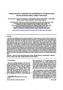
2. Damage Identification by ANNs The present research developed the damage quantification method by using multilayer perceptron feed-forward ANNs [10]. ANNs simulate the structure of the biological nervous system of the human brain and can provide a nonlinear mapping between a set of input data and a set of output data. ANNs consist of multiple layers including an input layer, hidden layer(s), and an output layer as shown in Figure 1, and these layers have nodes interconnected with the nodes of adjoining layers by synapses. 𝑆 in Figure 1 is the activation function which is chosen as the sigmoidal function as in 𝑆 (𝑎) =
1 , 1 + exp (−𝑎)
(1)
where 𝑎 is the input of the activation function. Each synapse has a weight called the synaptic weight which is updated by the supervised learning process that uses the 𝑁 pairs of a known set of input vectors {x𝑛 } (𝑛 = 1 ⋅ ⋅ ⋅ 𝑁) and a corresponding set of target vectors {t𝑛 } (𝑛 = 1 ⋅ ⋅ ⋅ 𝑁). This research has employed the backpropagation method [11] which is typically used for training ANNs. The backpropagation method changes the synaptic weight vector w to minimize recursively the sum squared error norm 𝐸 shown in 𝐸 (w) =
1 𝑁 2 ∑ y (x𝑛 , w) − t𝑛 , 2 𝑛=1
(2)
Shock and Vibration
3
Object bridge
FEM modeling of damaged bridge
FEM analysis
: measurement devices Vector expressing acceleration obtained by multipoint measurement (input data)
Vector expressing damage pattern Vector expressing damage pattern
1
2
.. . Vector expressing damage pattern
Target vectors
N
Vector expressing acceleration results at measurement points Vector expressing acceleration results at measurement points .. . Vector expressing acceleration results at measurement points
Training set Training stage
Input vectors
1
Train ANNs
2
N
Vector expressing damage pattern (output data)
: damage quantification results (final goal) Inspection stage
Figure 2: Overview of the method developed in the present research.
where y is the vector of output variables. The weight vector w is adjusted iteratively based on 𝜕𝐸 + 𝛼Δw(𝑟−1) ) , w(𝑟+1) = w(𝑟) + (−𝜂 (3) 𝜕𝑤 𝑤=𝑤(𝑟) where 𝜂 is defined as the learning rate; 𝛼 is the acceleration coefficient; and 𝑟 in the parenthesis is the iterative number. In this research, 𝜂 and 𝛼 are 0.2 and 0.8, respectively. Due to the accuracy, versatility, and robustness of the ANNs trained by the backpropagation method, ANNs have been applied to a variety of problems including pattern recognition, data mining, and image processing. Figure 2 shows a well-rounded picture of the method developed in this research. First of all, as shown in the leftside of Figure 2 (described as the “training stage”), ANNs are trained using a training set which explains the relation between the damage pattern and the acceleration characteristics at multiple measurement points. In this research, the acceleration characteristics are maximum values and variance of acceleration along the gravity direction calculated from the time-series vibration signal. To develop performance of ANNs, many training sets are required. However, because it is not easy to obtain many pairs of measurement results and damage assessments from actual bridges, the present research has employed FEM analysis, by which a bridge model with arbitrary corrosion damage can be made and analyzed easily. Then, the trained ANNs can be used to quantify the damage severity of an actual bridge as in the right-side of Figure 2 (described as the “inspection stage”). By inputting the acceleration characteristics obtained from multipoint
measurement results to the trained ANNs, it is expected to be possible to identify the location and degree of damage reasonably well. In this framework, the kind of acceleration characteristics used affects the performance. This research uses a maximum value and variance of acceleration calculated from time-series data at multiple measurement points caused by impact load as the acceleration characteristics.
3. Development of the Measurement Device Multipoint measurement results are required for the method developed in the present research as shown in Figure 2. However, it is not easy to prepare a number of commercial accelerometers for the multipoint measurement of small to midsized bridges because the inspection cost should not be very high for those bridges. We therefore developed the portable MEMS accelerometer shown in Figure 3 along with the wiring diagram. The MEMS accelerometer consists of a credit card sized single-board computer Raspberry Pi Model B+ (Raspberry Pi Foundation, 700 MHz CPU, and 512 MB RAM), an MMA8451Q 3-axis accelerometer (Freescale, output data rates being 800 Hz, 14 bit resolution, and selectable scale of ±2 g/±4 g/±8 g), microSDHC card (Transcend, memory size of 2 GB), and mobile battery QE-QL202X (Panasonic, 5,800 mAh battery capacity). The MEMS accelerometer runs for more than 24 hours on a single charge. It is controlled by the python program run by the Raspberry Pi, and for the reference of the reader, the authors provide the source code on their website (http://www.mech .cee.ehime-u.ac.jp/∼chun/acceleration raspberry.py). Since the MEMS accelerometer developed here is much cheaper
Shock and Vibration
1 2 3 4
(a)
MMA8451Q
4
5 6 7 8
(b)
Figure 3: Portable MEMS accelerometer and wiring diagram developed in the present research. 33300
48000
55500
42950
Span 1
Span 2
Span 3
Span 4
A1 M
M
P1
M
M
P2
F A2
P3
M Movable support F Fixed support
Figure 4: Side view of bridge H (unit: mm). Red circles indicate the points where strain was measured.
than that offered commercially, it can be used without entailing a large cost for the multipoint measurement. Specifically, the cost of making one unit is only 5500 JPY (47 USD at the date of January 21, 2015), which is less than 1/50 the cost of the commercial accelerometer owned by the authors. In addition, because the MEMS sensor is portable, it can be reused, which is also expected to reduce costs. Moreover, the device can be made only by building products freely available on the market; therefore it is easy to reproduce by anyone.
250
250 500
8500
500 805 120 305 2700
4. Example Application This chapter describes an application example of the developed method described above. According to a visual inspection, abnormal rust can be observed on bridge H. Therefore, the authors are planning to conduct a long-term followup inspection using the developed method to quantify the damage severity, especially in terms of thickness reduction due to corrosion. 4.1. Dimensions of Bridge H and Future Prediction Based on the Inspection Results. Bridge H is a four-span bridge constructed in 1992 and has four weathering steel I-girders supporting a 305 mm concrete deck as in Figures 4 and 5.
2500 × 3 = 7500
Figure 5: Cross-section drawing of bridge H (unit: mm).
Bridge H is located at a height of 200 m above sea level, and an antifreezing agent is used. As in Figure 6, another bridge is located below bridge H, and the antifreezing agent on the bridge is blown onto the external girder (girder G4) of bridge H due to the valley wind, and this causes severe damage to the girder. It is known that the corrosion damage on weathering steel reduces the thickness very much, which in turn reduces the load bearing capacity. Therefore, to clarify the condition
Shock and Vibration
5 Wind Bridge H
Blown antifreezing agent
Damage at G4 girder Ground Bridge H
(a)
(b)
Figure 6: Panoramic view of the exterior beam of bridge H (a) and the mechanism by which the G4 girder is corroded (b).
The work in [13] states that the thickness reduction does not follow a normal distribution but follows the lognormal distribution. The measurement results conducted by the authors after 20 years of exposure, as shown in Figure 8, also support a lognormal distribution of thickness reduction. As shown in Figure 8(b), the histogram of thickness reduction is not distributed symmetrically, and lognormal distribution fits the histogram better than normal distribution in such a case. The lognormal distribution is expressed as 2
𝑓 (𝑥) = Figure 7: Photos of the bottom flange of the G4 girder at span 2, at which the appearance rating is 2.
of bridge H, a visual examination based on the inspection manual (Table 1) developed by three organizations (the Public Works Research Institute of Japan’s Construction Ministry, the Japan Association of Steel Bridge Construction, and the Kozai Club [12]) was conducted in 2012. Then we found that appearance rating 2, which means severe corrosion damage, was seen on the bottom flange of the G4 girder of span 2. Figure 7 shows a picture of the damaged place. As for the other members, the appearance ratings were from 3 to 5, which means that the members may be safe. It is reported in [12] that the thickness reduction rate differs depending on the appearance grade determined by visual inspection. The above described three organizations have suggested the following equation to predict the thickness reduction based on the exposure test data of 41 weathering steel bridges in Japan: 𝑌 = 𝐴𝑋𝐵 ,
(4)
where 𝑋 is bridge age in years, 𝑌 is the thickness loss (mm), and 𝐴 and 𝐵 are corrosion rate parameters. The work in [12] showed 𝐴 and 𝐵 of the 41 bridges along with the appearance ratings evaluated by Table 1. From there, the mean and standard deviations of the amount of thickness reduction disaggregated by the appearance ratings of 1 to 5 can be derived as in Table 2.
(ln 𝑥 − 𝜇) 1 ), exp (− √2𝜋𝜎𝑥 2𝜎2
(5)
where 𝑥 is the random variable, which is the thickness reduction in this research. 𝜇 and 𝜎 are the location parameter and scale parameter, respectively. These parameters are derived from mean 𝑚 and standard deviation 𝑠 as in the following equations: 𝜇 = ln 𝑚 −
ln (𝑚2 /𝑠2 + 1) 2
𝑚2 𝜎 = √ ln ( 2 + 1). 𝑠
, (6)
Figure 9 shows the lognormal distribution of the thickness reduction of appearance ratings 2 to 4 which can be seen at bridge H at the bridge age of 50 years. As in the figure, the worse the appearance grade is, the greater the thickness reduction will be. The 99% two-sided confidence interval of appearance rating 2 is between 0.07 mm and 18.06 mm. This range is used in a later chapter. 4.2. Development of the FEM Model of Bridge H and Its Validation by a Vehicle Loading Test. As described above and in Figure 2, FEM results are used as training data of ANNs. For that purpose, the commercial FEM program Abaqus/Standard 6.14 (Dassault Syst`emes) was used to model and analyse bridge H. Figure 10 shows an isometric view of the FEM mode. The material properties of the concrete and weathering steel used here are shown in Table 3. In the model, the eightnode isoparametric brick element C3D8R was used for the
6
Shock and Vibration Table 1: Appearance ratings based on corrosion characteristics.
Appearance rating
Corrosion type
Grain size
Corrosion thickness
Color tone
1 (worst)
Laminated flaky corrosion
Larger than 25 mm
Thicker than 800 𝜇m
Varying color tone
2
Imbricate corrosion
5 mm to 25 mm
400 𝜇m to 800 𝜇m
Varying color tone
3
Abnormal corrosion of the early phase
1 mm to 5 mm
Thinner than 400 𝜇m
Varying color tone
4
Protective lust layers
Smaller than 1 mm
Thinner than 400 𝜇m
Dark brown
5 (best)
In the early stage of the formation of protective lust layers
Smaller than 1 mm
Thinner than 200 𝜇m
Light brown
Instance of appearance
15
Frequency
10
5
0 0.0 (a)
0.5 1.0 1.5 Thickness reduction (mm)
2.0
(b)
Figure 8: Photo of exposure test (a) and histogram of thickness reduction after 20 years of exposure (b).
concrete deck, and a shell element with reduced integration S4R was used for the steel girders and cross frames. The number of nodes and elements were 46,580 and 27,172, respectively. To demonstrate the validity of the FEM model, a live load test involving use of a sprinkler truck as shown in Figure 11
was conducted, and the strain at the bottom flange of the G4 girder of span 2 was measured. We measured two points: one at the distance of 8 m from P1 pier and the other at the center of span 2. For reference, red circles to indicate these points are drawn on Figure 4. The measurement frequency was 100 Hz. The truck was driven six times over the bridge to
Shock and Vibration
7 Table 4: Comparison of the first natural frequency between the live load tests and FEM analysis.
Probability density
8
6
Test 4 Test 5 Test 6 FEM
4
2
0
1
0
2 3 Thickness reduction (mm)
4
Rating 2 Rating 3 Rating 4
Figure 9: Probability density function of the thickness reduction with differing appearance ratings.
Figure 10: Isometric view of the FEM model of bridge H. Table 2: Mean and standard deviations of thickness reduction at the bridge age of 50 years disaggregated by appearance rating. (As for appearance rating 5, because only one bridge was tested, the standard deviation is not included in the table.) Appearance rating 1 2 3 4 5
Mean thickness reduction at the bridge age of 50 years
Standard deviation of thickness reduction at the bridge age of 50 years
8.27 mm 2.03 mm 0.32 mm 0.20 mm 0.12 mm
11.37 mm 2.98 mm 0.14 mm 0.05 mm N/A
Table 3: Material properties of concrete and weathering steel.
Young’s modulus Poisson’s ratio Density
Concrete 25 GPa 0.17 2.3 × 10⁻⁹ ton/mm3
Weathering steel 200 GPa 0.3 7.8 × 10⁻⁹ ton/mm3
maximize the bending moment of the G4 girder. The speed of the truck in the first three tests was 5 km/h to 15 km/h so that the dynamic effect could almost be removed, and these results were used to compare the static behavior between the
First natural frequency 3.27 Hz 3.27 Hz 3.32 Hz 3.31 Hz
live load test and the FEM result. The comparison results are shown in Figure 12. The horizontal axis indicates the distance between the edge of span 2 and the front axle, and the vertical axis indicates the strain. Considering the figure, it is safe to say that the FEM result shows good results in that the maximum strain of the FEM result is within the range of the three test results and the shape of the strain curve of the FEM result is similar to that of the test results. On the other hand, the truck speeds in the other three tests were 30 km/h (Test 4) and 50 km/h (Tests 5 and 6) and these results were used to compare the first natural frequency. The test result is shown in Figure 13 and the first natural frequency calculated from the measurement results is shown in Table 4. Table 4 also includes the first natural frequency calculated by FEM analysis for comparison. As shown in the table, the first natural frequency of the FEM result is in reasonable agreement with the live load tests; that is, the FEM result is within the range of live load test results. From these comparison results, it is safe to say that our FEM model is well-verified, and the model is used for further analysis in the next section. 4.3. Training ANNs by FEM Results. This section trains the ANNs by using the FEM results of damaged bridges. Here we modeled the damage only to the bottom flange of the G4 girder at span 2, of which the appearance rating was 2 because it is considered that the thickness of the other members, with an appearance grade more than 3, will not decrease very much in the future. Specifically, the average thickness reduction is only 0.32 mm and 0.20 mm for ratings 3 and 4, which are very small in comparison to the original thicknesses of 19 mm to 32 mm. Figure 14 shows the dimensions of the bottom flange of G4 of span 2. The bottom flange is broken down into seven parts as shown in the figure, from 𝑝1 to 𝑝7 . Then, different random thickness reductions 𝑑1 to 𝑑7 are given to 𝑝1 to 𝑝7 in the FEM model, respectively. The range of 𝑑1 to 𝑑7 is 0.073 mm∼18.062 mm, which is the 99% two-sided confidence interval of rating 2. In future inspections, we are planning to apply the impact force to the deck above the center of the G4 girder using our falling weight impact tester which drops a 20 kg weight from a height of 1.2 m. We simulate the impact force also in the FEM analysis. From the analysis, maximum value and variance of acceleration along the gravity direction are obtained from the time-series data at 18 measurement points (𝑚1 ⋅ ⋅ ⋅ 𝑚18 ) in Figure 14. Since plenty of data is required to train the ANNs appropriately, the present study develops 1500 FEM-damaged bridge models, changing 𝑑1 to 𝑑7 in the FEM models randomly, and then explicit analysis is carried out.
8
Shock and Vibration 40.18 kN 40.18 kN 40.18 kN 40.18 kN (rear) 1.32 m 14.30 kN
4.2 m
14.30 kN 2.45 m (front) (a)
(b)
Figure 11: Sprinkler truck used for live load test. 50 40
20
Microstrain
Microstrain
30 20 10
10
0 0 −10 −20
0
20
40
60
−10
0 10 20 30 Distance between front wheel and P1 (m)
Distance between front wheel and P1 (m) Test 2 Test 3
FEM Test 1
40
Test 2 Test 3
FEM Test 1
(a)
(b)
Figure 12: Comparison between live load tests (vehicle speed is 5 km/h to 15 km/h) and FEM analysis.
Table 5: The number of elements in the input and target vectors.
Input vector Target vector
The number of elements in the vector 2 × 18 = 36 (maximum value and variance of acceleration at 𝑚1 to 𝑚18 ) 7 (𝑑1 to 𝑑7 )
From the analysis, we get input and target data as in Table 5, and these data are used to train the ANNs. We also need to determine the number of hidden layers and nodes in the layers. In the application example, the number of hidden layers is set to 1, and the number of nodes in the hidden layer is 20, which is about half the number of nodes of the input layer and of the output layer. 4.4. Discussion on Accuracy. The accuracy of the method is discussed in this section. Note that this research conducted the ANN-based damage quantification only numerically because the damage to bridge H is not yet severe; that is, the thickness reduction is very small. Nonetheless, numerical analysis is meaningful for planning future inspections
because it is too late to develop the plan after the corrosion damage becomes severe. This paper confirms the accuracy of the developed method by the leave-one-out cross validation as in Figure 15. First of all, the accuracy of the prediction of thickness reduction is confirmed (“Comparison (1)” in Figure 15). Figure 16 shows a histogram of the error calculated by the following equation, which is the mean squared error: 1 7 2 error = √ ∑ (𝑑𝑖 target − 𝑑𝑖 output ) , 7 𝑖=1 target
output
(7)
where 𝑑𝑖 and 𝑑𝑖 are the 𝑑𝑖 of the target and output data, respectively. According to the calculation, it is found that the average of the mean squared error of the amount of thickness reduction is only 0.2 mm. Figure 17 shows an example of the calculation results which are randomly picked up. As shown in the figure, the damage was properly evaluated, and the same conclusion can be obtained from the other cases.
9
50
40
40
30
30 Microstrain
50
20
20 10
10
0
0 −10
−10
0
5
10
15
20
0
5
10 Time (s)
Time (s) Point A Point B
15
Point A Point B (a) Test 4 (30 km/h)
(b) Test 5 (50 km/h)
50 40 30 Microstrain
Microstrain
Shock and Vibration
20 10 0 −10
0
5
10 Time (s)
15
20
Point A Point B (c) Test 6 (50 km/h)
Figure 13: Results of live load tests with higher speed ((a): 30 km/h, (b) and (c): 50 km/h) used to derive natural frequency.
1960 3700 m1 m2
m3
Part 1 (p1 ) Original thickness 28 mm Thickness reduction d1 mm Max width 530 mm
6700 m4
m5
Part 2 (p2 ) Original thickness 25 mm Thickness reduction d2 mm Max width 450 mm
m6
10900 m7 m8 Part 3 (p3 ) Original thickness 19 mm Thickness reduction d3 mm Max width 340 mm
m9
m10
Part 4 (p4 ) Original thickness 25 mm Thickness reduction d4 mm Max width 610 mm
10900 m11 m12
m13
Part 5 (p5 ) Original thickness 25 mm Thickness reduction d5 mm Max width 610 mm
m14
11602 m15 m16
Part 6 (p6 ) Original thickness 28 mm Thickness reduction d6 mm Max width 580 mm
Figure 14: Dimensions of bottom flange of G4 girder of span 2 (unit: mm).
m17
2138 m18
Part 7 (p7 ) Original thickness 32 mm Thickness reduction d7 mm Max width 670 mm
20
10
Shock and Vibration Select one of the sets and calculate N times
{ Input data1 , Target data1 } { Input data2 , Target data2 } .. . { Input datak−1 , Input datak−1 }
{ Input datak , Target datak } FEM
Training by N − 1 ANNs Comparison (1) Comparison (2) sets of data FEM Output datak }
{ Input datak+1 , Input datak+1 } .. . { Input dataN , Target dataN Training data sets
Input data : acceleration characteristics at 18 measurement points Target data , Output data : amount of thickness reduction at 7 parts
Figure 15: Validation of developed method by leave-one-out cross validation.
Frequency
600
400
200
0 0.0
0.5
1.0
1.5
2.0
Root mean squared error (mm)
Figure 16: Histogram of root mean squared error of thickness reduction obtained from leave-one-out cross validation.
Original thickness
d1 28 mm
d2 25 mm
d3 19 mm
d4 25 mm
d5 25 mm
d6 28 mm
d7 32 mm
Error by Eq. (7)
Example dataset 2
Target 27.46 mm 23.58 mm 16.82 mm 23.10 mm Output 27.12 mm 23.21 mm 15.99 mm 24.21 mm Target 27.32 mm 23.42 mm 18.18 mm 24.13 mm Output 26.89 mm 23.12 mm 17.89 mm 24.22 mm
Example dataset 3
Target 26.95 mm 13.14 mm 18.27 mm 14.63 mm 23.00 mm 20.25 mm 27.39 mm 0.42 mm Output 26.89 mm 13.21 mm 17.91 mm 15.38 mm 23.64 mm 20.53 mm 27.20 mm
Example dataset 1
13.04 mm 25.25 mm 29.66 mm 14.23 mm 25.31 mm 29.23 mm 24.60 mm 25.75 mm 31.21 mm 24.24 mm 25.89 mm 30.99 mm
0.73 mm 0.28 mm
Figure 17: Comparison example between target data and output data.
Both the accuracy of the thickness reduction prediction and the accuracy of the mechanical behavior prediction are confirmed here. The 1500 sets of 𝑑1 to 𝑑7 of the target data and output results by ANNs are given to the FEM model, and the maximum stress along the traffic direction at the bottom flange of G4 girder of span 2 (“Comparison (2)” in Figure 15) is compared. Loads applied to the model are design dead load and live load to maximize the bending moment at span 2. These loads are determined in accordance with the specifications for highway bridges in Japan [14]. Figure 18 shows the live load on span 2 and span 4. Note that live load is not applied on spans 1 and 3 because these loads reduce the bending moment at span 2. Figure 19 is a histogram showing how much the maximum stress differs between the target data
and the output data. The average and standard deviations of error are only −0.0028% and 0.4507%, respectively. Therefore it is reasonable to say that the damage evaluation method developed here has enough accuracy to determine the safety of the structure and to decide whether maintenance action is required or not.
5. Concluding Remarks An ANNs-based damage severity quantification method which is categorized as level 3 by Rytter’s classification is proposed in this paper. In addition, an application example of the method to bridge H is also presented here. The method is
Shock and Vibration
11
8.5 m
19 m
10 m
19 m
4.214 kN/m2
16.255 kN/m2
4.214 kN/m2
2.107 kN/m2
8.127 kN/m2
2.107 kN/m2
G4 girder G1 girder
(a)
42.95 m 8.5 m
4.214 kN/m2
G4 girder
2.107 kN/m2
G1 girder
(b)
Figure 18: Design live load on span 2 (a) and span 4 (b). 600
References
500
[1] T. Kitada, “Considerations on recent trends in, and future prospects of, steel bridge construction in Japan,” Journal of Constructional Steel Research, vol. 62, no. 11, pp. 1192–1198, 2006. [2] Ministry of Land-Infrastructure-Transport and Tourism of Japan, 2014 Roads in Japan, Ministry of Land, Infrastructure, Transport and Tourism of Japan, Tokyo, Japan, 2014, http:// www.mlit.go.jp/road/road e/pdf/ROAD2014web.pdf. [3] American Society of Civil Engineers, “2013 Report Card for America’s Infrastructure,” 2013, http://www.infrastructurereportcard.org/a/#p/bridges/overview. [4] O. S. Salawu, “Detection of structural damage through changes in frequency: a review,” Engineering Structures, vol. 19, no. 9, pp. 718–723, 1997. [5] P. C. Chang, A. Flatau, and S. C. Liu, “Review paper: health monitoring of civil infrastructure,” Structural Health Monitoring, vol. 2, no. 3, pp. 257–267, 2003. [6] A. Rytter, Vibration based inspection of civil engineering structures [Ph.D. thesis], University of Aalborg, Aalborg, Denmark, 1993. [7] T. Nagayama, P. Moinzadeh, K. Mechitov et al., “Reliable multihop communication for structural health monitoring,” Smart Structures and Systems, vol. 6, no. 5-6, pp. 481–504, 2010. [8] S. Hara, T. Kamimura, H. Miyuki, and M. Yamashita, “Taxonomy for protective ability of rust layer using its composition formed on weathering steel bridge,” Corrosion Science, vol. 49, no. 3, pp. 1131–1142, 2007. [9] H. Kihira, “Development of corrosion prediction software for designing weathering steel structures with semi-eternal service life,” Nippon Steel Technical Report 87, Nippon Steel, 2003. [10] C. M. Bishop, Pattern Recognition and Machine Learning, Springer, New York, NY, USA, 2006. [11] D. E. Rumelhart, G. E. Hinton, and R. J. Williams, “Learning representations by back-propagating errors,” Nature, vol. 323, no. 6088, pp. 533–536, 1986. [12] The Public Works Research Institute of the Japan’s Construction Ministry, The Japan Association of Steel Bridge Construction, and The Kozai Club, “Report on application of weathering steel to highway bridges (XV),” Tech. Rep. 71, PWRI, 1992. [13] A. Rao, M. Lepech, and A. S. Kiremidjian, “Time-dependent earthquake risk assessment modeling incorporating sustainability metrics,” in Life-Cycle of Structural Systems: Design, Assessment, Maintenance and Management, pp. 50–69, 2014. [14] Japan Road Association, Specifications for Highway Bridges, Maruzen, 2002.
Frequency
400 300 200 100 0
−4
−2
0 Error (%)
2
4
Figure 19: Histogram of the error of maximum stress on the G4 girder obtained from leave-one-out cross validation.
planned to be employed to evaluate the thickness reduction due to corrosion as part of a long-term damage evaluation follow-up plan. In the application example, FEM results were used to train the ANNs, and the accuracy of ANNs is confirmed by leave-one-out cross validation. It was found that the proposed method could evaluate the location and degree of damage well. Furthermore, by using FEM, the accuracy of maximum stress prediction was also validated, which in turn helps us to evaluate the safety of the structure and develop appropriate maintenance strategies. For further work, it is suggested to validate the proposed method using actual damaged bridges because the present study validates the method only numerically. While it would be best to validate the method using actual data concerning bridge H, it will take several years or maybe even decades before thickness reduction becomes obvious. Therefore, we will attempt to validate the method using a scaled damaged bridge model, and this will be reported in our next paper.
Conflict of Interests The authors declare that there is no conflict of interests regarding the publication of this paper.
International Journal of
Rotating Machinery
Engineering Journal of
Hindawi Publishing Corporation http://www.hindawi.com
Volume 2014
The Scientific World Journal Hindawi Publishing Corporation http://www.hindawi.com
Volume 2014
International Journal of
Distributed Sensor Networks
Journal of
Sensors Hindawi Publishing Corporation http://www.hindawi.com
Volume 2014
Hindawi Publishing Corporation http://www.hindawi.com
Volume 2014
Hindawi Publishing Corporation http://www.hindawi.com
Volume 2014
Journal of
Control Science and Engineering
Advances in
Civil Engineering Hindawi Publishing Corporation http://www.hindawi.com
Hindawi Publishing Corporation http://www.hindawi.com
Volume 2014
Volume 2014
Submit your manuscripts at http://www.hindawi.com Journal of
Journal of
Electrical and Computer Engineering
Robotics Hindawi Publishing Corporation http://www.hindawi.com
Hindawi Publishing Corporation http://www.hindawi.com
Volume 2014
Volume 2014
VLSI Design Advances in OptoElectronics
International Journal of
Navigation and Observation Hindawi Publishing Corporation http://www.hindawi.com
Volume 2014
Hindawi Publishing Corporation http://www.hindawi.com
Hindawi Publishing Corporation http://www.hindawi.com
Chemical Engineering Hindawi Publishing Corporation http://www.hindawi.com
Volume 2014
Volume 2014
Active and Passive Electronic Components
Antennas and Propagation Hindawi Publishing Corporation http://www.hindawi.com
Aerospace Engineering
Hindawi Publishing Corporation http://www.hindawi.com
Volume 2014
Hindawi Publishing Corporation http://www.hindawi.com
Volume 2014
Volume 2014
International Journal of
International Journal of
International Journal of
Modelling & Simulation in Engineering
Volume 2014
Hindawi Publishing Corporation http://www.hindawi.com
Volume 2014
Shock and Vibration Hindawi Publishing Corporation http://www.hindawi.com
Volume 2014
Advances in
Acoustics and Vibration Hindawi Publishing Corporation http://www.hindawi.com
Volume 2014