Bridging the Gap Between Design and ... - Semantic Scholar

48

IEEE TRANSACTIONS ON AUTOMATION SCIENCE AND ENGINEERING, VOL. 11, NO. 1, JANUARY 2014

Bridging the Gap Between Design and Implementation of Discrete-Event Controllers Marcos Vicente Moreira and João Carlos Basilio, Member, IEEE

Abstract—Extended labeled Petri nets (ELPNs), i.e., labeled Petri nets with inhibitor arcs, are usually used to model the desired closed-loop behavior of a controlled discrete-event system, and, as such, their states are formed with both the controller and the plant states. However, the control logic is based on the controller states only and the interaction between controller and plant is carried out through sensor readings from the plant and control actions (forced events) from the controller. This makes ELPN not suitable for modeling the controller. Control interpreted Petri nets (CIPNs), on the other hand, include control actions in the places and sensor readings in the transitions as part of their formal structure, and so provide a better formalism for controller modeling. In this paper, we propose a two-step approach to discrete-event controller implementation, as follows: (i) we first propose a set of transformation rules to convert the initial ELPN to an equivalent CIPN, therefore extracting the control logic from the desired closed-loop behavior and (ii) we present a straightforward systematic way to translate the CIPN into a ladder diagram. We apply the results presented here to the implementation of the automation system of a plastic molding machine. Note to Practitioners—The usual approach to the design of manufacturing systems is to model the desired closed-loop system behavior using, for example, Petri nets, and in the sequel to extract the discrete-event controller from this model with the view to implementing the control logic on a Programmable Logic Controller (PLC). So far, the controller extraction is carried out in an ad hoc and intuitive way. In order to overcome the lack of formal methods to deal with controller extraction and implementation, we propose here a set of rules to construct, in a systematic way, the ladder diagram that implements the discrete-event controller. We illustrate the conversion technique proposed here by applying it to the implementation of the automation system of a plastic molding machine. Index Terms—Discrete-event systems (DESs), ladder diagram, manufacturing systems, Petri nets, programmable logic controller (PLC).

I. INTRODUCTION

P

ETRI NET [1]–[3] is one of the formalisms that is suitable to model and visualize the behavior of discrete-event systems (DESs). They have recently been applied successfully to

Manuscript received February 09, 2013; revised May 27, 2013; accepted August 17, 2013. Date of publication October 04, 2013; date of current version January 01, 2014. This paper was recommended for publication by Associate Editor C. N. Hadjicostis and Editor M. C. Zhou upon evaluation of the reviewers’ comments. The work of J. C. Basilio was supported in part by the Brazilian Research Council (CNPq), under Grant 306592/2010-0. The authors are with the COPPE-Programa de Engenharia Elétrica, Universidade Federal do Rio de Janeiro, 21949-900, Rio de Janeiro, RJ, Brazil (e-mail: [email protected]; [email protected]). Color versions of one or more of the figures in this paper are available online at http://ieeexplore.ieee.org. Digital Object Identifier 10.1109/TASE.2013.2281733

several problems ranging from manufacturing systems to web applications [4]–[6]. Among the advantages of Petri nets we may list their capacity to model behaviors such as concurrency, synchronization, and resource sharing. Other advantages of Petri nets include the possibility to describe both the desired closed-loop behavior of controlled DES and its discrete-event controller (DEC). Several methods have been proposed to synthesize DECs. Holloway et al. [7] distinguishes three main approaches: (i) the control theoretic approach [8]–[10]; (ii) the logic controller approach [11]–[13]; and (iii) the controlled behavior approach [14]–[16]. In the logic controller approach, the objective is to directly design a controller defining its input–output behavior, in order to achieve the desired controlled behavior for the closedloop system. This method can be applied to the control of simple processes, and simulation is necessary for the validation of the closed-loop behavior. The controlled behavior approach, on the other hand, is preferable for the design of complex manufacturing systems and consists of modeling the desired closed-loop system behavior, namely, the joint model of the plant and controller, and then to extract the DEC for implementation. This strategy allows properties of interest such as liveness, boundedness, and reversibility to be guaranteed or even previously analyzed using the desired closed-loop model. In using the controlled behavior approach, the desired closedloop behavior of the controlled DES is usually modeled with extended labeled Petri nets (ELPNs), i.e., labeled Petri nets with inhibitor arcs, and, as such, their states are formed with both the controller and the plant states. However, the control logic is based on the controller states only and the interaction between controller and plant is carried out through sensor readings from the plant and control actions (forced events) from the controller. This makes ELPN not suitable for modeling the controller. Control interpreted Petri nets (CIPNs) [17]–[20], on the other hand, include control actions in the places and sensor readings in the transitions as part of their formal structure, and so provide a better formalism for controller modeling. After a CIPN, that models the controller, has been obtained from the ELPN that models the desired closed-loop behavior of the DES, the next step is to generate a code for implementation on a programmable logic controller (PLC) by converting the control logic described by the CIPN into a PLC programming language, e.g., Sequential Function Charts (SFC) [21], [22] or Ladder diagrams [18], [20], [23]–[25]. In [20], a comprehensive survey about methods for the design and implementation of DECs using ladder diagrams and Petri nets is presented. Some of the techniques reviewed in [20] consist of designing and converting Petri nets (or extensions of Petri nets) to ladder diagrams for PLC implementation. How-

1545-5955 © 2013 IEEE

MOREIRA AND BASILIO: BRIDGING THE GAP BETWEEN DESIGN AND IMPLEMENTATION OF DECS

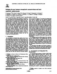
Fig. 1. (a) CIPN where only transition is enabled and (b) incorrect state reached after the occurrence of event when the avalanche effect occurs in the controller code.

ever, there is an important problem that may appear in the implementation of controllers in ladder diagrams: the avalanche effect. The avalanche effect occurs in the PLC implementation of the Petri net controller when the receptivities of two or more consecutive transitions become true at the same scan cycle and, in the controller code, transitions that were not enabled are incorrectly transposed. For example, consider the Petri net of Fig. 1(a). In this case, if event occurs, only transition must fire since only is enabled. Transition will fire only after the second occurrence of event . However, depending on the programming code, both transitions can be transposed in the same scan cycle, leading to the state of the Petri net of Fig. 1(b), which is not the intended behavior of the controller. The earliest conversion methods were based on the so-called Token Passing Logic (TPL) technique [18], [23], whose idea was to use the evolution of the tokens through the Petri net as the main mechanism for controlling the flow of the control logic. Although the methods proposed in these papers were successfully implemented on manufacturing systems, the avalanche effect was not explicitly considered. The avalanche effect was addressed for the first time in [21], who proposed a systematic procedure for avoiding it in ladder implementations of supervisory control systems modeled using automata. The only drawback of the approach presented in [21] is the lack of a formal method to deal with cycles, namely, where to break the loop in an intelligent way for implementation purpose. Jimenez et al. [26] consider the conversion of timed interpreted Petri nets into ladder diagrams. In the method proposed in [26], each transition in the net is translated into a network in the ladder diagram. Differently from [18] and [23], the method presented in [26] cannot be applied to extended Petri nets. It is worth mentioning that the avalanche effect was not addressed in [26] either. In [24], a different approach was proposed as follows: first, Boolean expressions are obtained from the CIPN, and then, these expressions are straightforwardly converted into a ladder code. The weakness of this technique is that the resulting ladder diagram does not provide a simple visualization of the control code, and thus, simple modifications in the control logic cannot be easily implemented in the existing ladder diagram.

49

In [27], the implementation on PLCs of Ramadge–Wonham (RW) supervisors [28] with time delay functions is considered and a method, based on the TPL technique, is proposed for obtaining a ladder diagram from the supervisor. The avalanche effect and other problems associated with the implementation of supervisors on PLC have not been addressed. In [29], a hierarchical control of DESs is proposed. In a lower level, a DEC is designed to force control events to occur and, in a higher level, a supervisor prohibits the occurrence of some events such that the closed-loop system satisfies the specifications given by the designer. The main advantage of this hierarchical frame is that the control and supervision tasks are clearly separated. This strategy has been named as the supervised control of DESs. The supervision and control are both designed in [29] by using GRAFCET. In [30], the implementation of the supervised control in structured text (ST)—one of the five PLC languages defined in the standard IEC 61131-3 [31]—is addressed. First, the system is partitioned into several subsystems, each one having a DEC that performs only simple sequences, with no resource sharing; in this approach, the control logic must be very simple in such a way that the controller can be directly implemented on a PLC. Then, the coordination of the subsystems is managed by a supervisor designed by using the RW supervisory control theory. An evolution algorithm for the implementation of supervisors, and a set of rules for the translation of the supervisor described by automata or Petri nets into an ST code were proposed in [30]. Although the algorithm proposed in [30] avoids the avalanche effect, the method does not approach the implementation of complex DECs with conflicts and resource sharing, and also do not consider DEC modeled by CIPNs and timed Petri nets. More recently, it has been shown in [32] that complex distributed control systems can be implemented by using IEC 61131 languages extended with object oriented programming. The avalanche effect was, again, considered in [25], for complex DEC modeled by timed CIPN. A conversion technique that establishes transformation rules from CIPN to ladder diagrams which preserve the structure of the Petri net and also avoids the avalanche effect were given in [25]. We assume here that the controlled behavior approach is the methodology used to synthesize the DEC. Thus, starting from the ELPN model of the desired closed-loop behavior, we will propose a two-step approach to the implementation of the DEC, as follows: (i) first, a set of transformation rules is used to convert the initial ELPN to an equivalent CIPN, therefore extracting the control logic from the desired closed-loop behavior and (ii) a straightforward systematic way, which is an extension of that proposed in [25], is given to translate the CIPN into a ladder diagram. The translation rules make use of the structure and dynamics of the Petri net to obtain conditions for the firing of transitions and to describe the flow of the control logic. The ladder diagram is built in such a way that the avalanche effect is avoided and its structure allows any modification in the DEC modeled by the CIPN to be easily implemented in the existing ladder diagram. It is worth remarking that, although several works address the problem of modeling closed-loop systems by using labeled Petri nets, from the authors’ knowledge, the problem of extracting a controller from this Petri net model using CIPN has not been addressed in the literature.

50


We present in Section II a brief review of Petri nets and in Section III we first introduce the definition of ELPNs, and, in the sequel, we define CIPNs. We propose in Section IV a set of transformation rules for obtaining a CIPN from an ELPN, and, in Section V, we introduce the method for obtaining the ladder diagram from the CIPN. We illustrate the methodology proposed here with the design of an automation subsystem of a plastic injection molding machine. We present concluding remarks in Section VI. II. PRELIMINARIES A Petri net graph is a bipartite graph that contains two types of nodes: places and transitions. The places are represented by circles and the transitions by bars, and these two types of nodes are connected through directed arcs. The formal definition of a Petri net graph is as follows. Definition 1: A Petri net graph is a weighted bipartite graph , where is the finite set of places, is the finite set of transitions, is the function of ordinary arcs that connect places to transitions, is the function of ordinary arcs that connect transitions to places. The set of input (output) places of a transition is denoted as , and is formed with places such that . Let denote the marking function. Then, represents the number of tokens assigned to place . A marking of a Petri net is the column vector formed with the number of tokens in each place , for , where is the cardinality of . Definition 2: A Petri net is a five-tuple , where is, in accordance with Definition 1, a Petri net graph, and is the initial marking function. A transition is said to be enabled when the number of tokens in each one of its input places is greater than or equal to the weight of the arcs connecting the places to transition , i.e., is enabled if and only if (1) If transition is enabled for a marking and fires, then a new marking is reached. The evolution of the markings is given by the following equation: (2) Finally, we say that a place is a safe place if for all markings of the Petri net reachable from . In order to use the Petri net formalism to model physical systems (e.g., manufacturing systems), it is necessary to label the transitions with events from an event set . This leads to the definition of labeled Petri nets, as follows [33]. Definition 3: A labeled Petri net (LPN) is a seven-tuple , where , is according to Definition 1, a Petri net graph, is the set of events for transition labeling, is the transition labeling function, and is the initial marking function of the system.

Now, let be the set of output transitions of a place . When is an input place of two or more transitions, we have a conflict. Three types of conflicts can be identified, as follows: • Structural conflict. A structural conflict, denoted by , exists when the cardinality of is greater than one. Notice that the existence of a structural conflict is independent of the Petri net marking. • Effective conflict. An effective conflict depends on the marking of the Petri net [3]. An effective conflict, denoted by is formed by a structural conflict and a marking , such that a subset of with at least two transitions are enabled by and the number of tokens in is smaller than the sum of the weights of all arcs connecting place to the enabled transitions of . • Actual conflict. An actual conflict is an effective conflict where the events associated with two or more enabled transitions of occur simultaneously. In the theory of supervisory control this case cannot happen since it is assumed that two distinct events never occur simultaneously. This is actually true when the events are independent [3]. However, PLCs update their inputs synchronously and even when the events are independent, they may be seen by the PLC as occurring at the same time [21]. The resolution of conflicts is not a trivial task in the design of DES and is beyond the scope of this paper. However, since we assume that the DEC synthesis is carried out by using the controlled behavior approach, it is very reasonable to assume that all possible conflicts have already been solved by the designer. We will therefore make the following assumption. A1) All the actual conflicts have been solved by the designer before the implementation of the controller, i.e., in the construction of the ELPN. III. EXTENDED LABELED AND CONTROL INTERPRETED PETRI NETS In this section, we will extend the definition of LPN, which will be used to model the desired behavior of a closed-loop DES, and, in the sequel, we will briefly review the concepts of CIPN, which will be used to describe the controller behavior. The two formalisms are related/interconnected in accordance with the block diagram shown in Fig. 2. A. Extended Labeled Petri Nets (ELPNs) The definition of ELPNs is as follows. Definition 4: An ELPN is an eight-tuple (3) where is, according to Definition 3, a labeled Petri net, and is the inhibitor arc function. The inhibitor arc function allows a larger class of DES to be represented, increasing the modeling power of the labeled Petri net. It can be used to eliminate conflicts since, if there is a inhibitor arc connecting a place to a transition , then transition will be disabled if the number of tokens in is greater than or equal to the weight of the arc that connects


Fig. 2. Closed-loop system.

to , i.e., . The inhibitor arc is graphically represented by a solid line terminating with a small circle. The desired closed-loop behavior of a large class of DES, mainly manufacturing systems, can be modeled by the ELPN introduced in Definition 4; for example, all Petri net models for manufacturing systems presented in [14] can be described by a labeled Petri net; it is worth remarking that all conflicts are avoided in [14] with the so-called choice-synchronization structure, which is a particular case of firing priority attribution. In [2] and [3], several DES modeled by ELPNs are presented. We say that a transition of an ELPN is observable if one of the following conditions associated with the labeling event holds true: (i) the event has a sensor to indicate its occurrence; (ii) the event is a command signal sent by the controller to the plant; (iii) the event is associated with a time delay; and (iv) the event is associated with the synchronization of internal conditions observable by the controller; for instance, the synchronization in the end of two concurrent processes that is verified by the controller to command the start of a third process. We will suppose in this paper that all transitions of the ELPN are observable by the controller. B. Control Interpreted Petri Nets (CIPNs) The CIPN has additional structures to deal with sensors and actuators. The inputs of the CIPN, associated with transitions, are signals sent from sensors to inform the occurrence of events, and the outputs, associated with places, are impulse actions commanded to the plant. In order to include timers, the CIPN is also T-timed. Therefore, the set of transitions of the CIPN, , can be partitioned as , where is the set of transitions with no firing delays and is the set of timed transitions. Definition 5: A CIPN is a 13-tuple (4) where is an extended Petri net, and are the sets of conditions and input events associated with the transitions in , respectively,

51

is the function that associates to each transition in an event from and a condition from , denotes the set of delays associated with timed transitions, is the timing function that associates to each timed transition a delay from , is the set of impulse actions, associated with safe places in , and is the action assigning function, where denotes the set of safe places. Notice in Definition 5 that it is assumed that every transition is associated with a condition in and an event in . Transition may fire when it is enabled and the associated condition is true, and fires when the associated event occurs. If the condition associated with is not explicitly specified, then the condition is equal to one, i.e., the logical condition is true. Moreover, if the input event is not explicitly specified, then the event is equal to , the always occurring event [3], to indicate that transition must fire immediately after it becomes enabled if the associated condition is true. Therefore, all transitions in have Boolean expressions associated with them. According to Definition 5, impulse actions are assigned to safe places in . If a place does not have an action associated with it, then , and if a place with assigned actions is marked, then the impulse actions are executed when place changes its marking from zero to one. It is important to remark that the impulse action must be executed even if the marking of place is unstable [3], i.e., it changes from zero to one and then back to zero instantaneously. Thus, the execution of the impulse actions are directly related to changes in the markings of the safe places where . The reason to consider only impulse actions comes from the fact that the CIPN is obtained from a labeled Petri net—all transitions are labeled with events whose occurrence are instantaneous. Thus, the controller command events, associated with the transitions in the labeled Petri net, can be seen as impulse actions. In order to consider also level actions, modifications should be applied to the final CIPN obtained by using the method proposed in this paper. These modifications will not be addressed here. In the following section, we show that it is always possible to extract a DEC, described by a CIPN satisfying Definition 5, from a closed-loop system modeled by an ELPN whose transitions are all observable by the controller. IV. CIPN EXTRACTION FROM AN ELPN We will now propose transformation rules to change ELPNs to CIPNs. The transformation will be carried out in two steps, as follows: first, transformations will be defined in such a way that the conditions imposed by Definition 5 are satisfied, leading therefore to a CIPN; then, the resulting CIPN will be modified so as to reduce the number of places and transitions. A. Transformation of an ELPN to a CIPN Let denote an ELPN defined according to Definition 4. Partition the event set of as

where denotes the set of actions, the set of events associated with time delays, the set of events observed by sensors, and the set of events associated with the synchronization of

52


place and transition sets. The Reduction rules proposed here are based on the reduction techniques used to mitigate the effort in the verification of Petri net properties [15], [34]–[37]; the difference is that here we are interested in guaranteeing that the discrete-event closed-loop system executes the correct sequence of events described by the ELPN. As in the reduction methods used to verify Petri net properties, the idea behind the reduction technique presented in this paper is to examine the Petri net structure and/or behavior and to apply appropriate Reduction rules to reduce the net size as much as possible [15]. It is worth mentioning that the application of a rule may lead to a modified CIPN that enables the application of another rule that was not possible before. Thus, the determination of a correct order for the application of the Reduction rules depends on the controller Petri net model. In each of the following subsections, a Reduction rule is applied to a CIPN, , generating a reduced CIPN (RCIPN) Fig. 3. (a) Transition labeled with a command event in an ELPN and (b) its expansion in a CIPN according to transformation rule T3.

internal conditions observable by the controller. A CIPN equivalent to the given ELPN is formed as follows: T1) Keep the set of places of in , i.e., . T2) Keep the transitions labeled with events in the set in . (a) For a transition such that , synchronizes the corresponding transition with the rising edge or the falling edge of the sensor signal. (b) For a transition such that , synchronizes the corresponding transition with the always occurring event . (c) For a transition such that , create a timed transition with the same delay time as described by the event of . (d) For each transition created in steps (a)–(c), define , , and , for all . T3) For a transition such that , create two transitions , both synchronized with , and a safe place such that , and define , , , for all , and . In addition, convert event to an impulse action associated with place . Fig. 3 illustrates transformation T3. For obvious reasons, the CIPN obtained according to transformation rules T1–T3 will be referred here to as direct control interpreted Petri net (DCIPN). B. Reducing the Size of CIPN The DCIPN obtained from the ELPN in the previous subsection is likely to have redundant places and transitions. Since controller implementation depends on the number of places and transitions, it would be worthwhile to carry out additional transformations in the DCIPN so as to reduce the cardinality of the

1) Recognizing a Condition for the Firing of a Transition Associated With a Sensor: In some cases, an ELPN is constructed in accordance with a bottom-up approach, in which, several components of the system are first modeled by Petri nets, and then these modules are appropriately connected in order to represent the coupling effects among them. Let us assume that and are two net components of an ELPN that satisfy the following conditions: C1.1—The places of represent only discretized states the component may achieve. C1.2—The transition from one state to another in can be observed by sensors. C1.3—The marking of a place in is one of the conditions for the firing of a transition in ; this is tantamount to saying that there is a self-loop between and . If conditions C1.1–C1.3 are satisfied, we can reduce the CIPN according to the following rule. Reduction Rule 1: 1) Eliminate the connection between the modules: (a) If is not a transition associated with an action, eliminate the self-loop between and in the CIPN, i.e., set , and add to a condition associated with a sensor ( or ). (b) If is associated with an impulse action, eliminate the arcs in the CIPN between and , and and , i.e., set , a condition associated with sensor and add to ( or ). 2) Keep the initial marking of the net, i.e., set . 3) Eliminate net component if it is isolated from the rest of the net and is not part of the control system, i.e., if it satisfies the following conditions: (a) None of its places has an assigned action. (b) None of its places is an input or output place of a transition of another module. (c) None of its transitions is an input or output transition of a place of a different module.


53

Fig. 5. (a) Part of a Petri net satisfying the conditions for the merging of transitions and (b) simplification by merging the transitions.

Fig. 4. (a) ELPN with two component models and ; (b) corresponding and , and DCIPN; (c) CIPN obtained after eliminating the arcs between and ; (d) elimination of the isolated module .

In Fig. 4(a), transition is labeled with an impulse action, and thus, applying the transformation rules T1–T3, the DCIPN of Fig. 4(b) is obtained. In this case, we can eliminate the arcs from to , and from to . Fig. 4(c) presents the resulting reduced CIPN. Notice that module in the resulting Petri net is isolated from the rest of the net and does not represent part of the control system, and thus, it can be eliminated, leading to the reduced net of Fig. 4(d). 2) Merging Transitions: The merge of two transitions , whose associated events and conditions are and , respectively, is possible if the following conditions are satisfied: C2.1—The receptivities and are mutually exclusive. C2.2— , for all . C2.3— , for all . C2.4— , for all . Notice, according to Assumption A1, that and cannot be conflicting transitions. Thus, requirement C2.1 is not conservative when and also satisfy C2.2, C2.3, and C2.4. The reduction creates a new transition , obtained after merging and , leading to a reduced net whose components are given as follows. Reduction Rule 2: 1) . 2) .

Fig. 6. (a) Part of an extended Petri net satisfying the conditions for the merging of transitions and (b) simplification by merging the transitions.

3) if if 4) if if

.

5) if if

.

. 6) 7) The event associated with is defined as . In Figs. 5(a) and 6(a), two transitions and satisfying conditions C2.1–C2.4 are presented. As shown in Figs. 5(b) and 6(b), a single transition synchronized with is obtained by applying Reduction rule 2. 3) Merging Parallel Places: Two places and can be merged if the following conditions are satisfied. C3.1—The set of input transitions of is equal to the set of input transitions of , . C3.2—The set of output transitions of is equal to the set of output transitions of , i.e., . C3.3—For each pair of transitions such that and , the following equation holds true: (5)

54


C3.4) The initial condition of

and

satisfies:

of an inhibitor arc in notice that, if

. In order to overcome this problem,

(6) where is an input transition of and . It is not difficult to see that if (5) is satisfied for all pairs of input and output transitions of and , then

where denotes the smallest integer value greater than or equal to , then condition (11) is verified. Moreover, it can be easily seen that, since is an integer value, if

(7) for all pairs , where rational numbers. Therefore

denotes the set of positive

then

(8) which implies that the new inhibitor arc weight in lent to in , is given by

and (9) According to (9), if an input transition fires then tokens are added to place and . On the tokens are added to place fires other hand, according to (8), if an output transition and tokens are removed from place then . In addition, if tokens are removed from will be proportional condition (6) is verified, the marking of for all reachable markings of the net, i.e., to the marking of

(12) and Now, consider the case when . In this case, there are two inhibitor conditions for the firing of transition , as follows: (13) and (14)

(10) Therefore, it is not necessary to consider both and to the control of the firing of their output transitions, and so, places and can be merged, preserving the transition firing sequences of the net. If there is an inhibitor arc from place and/or to a transition , and conditions C3.1–C3.4 are true, then it is necessary to define appropriately the weight of the inhibitor arc from the merged place to . Let us first consider the case when and . In this case two possibilities arise: (i) if , then , since the marking of will be equal to the marking of for all reachable states of the Petri net and (ii) if , then the weight of the inhibitor arc can be different from since for all reachable states of the net, and, according to (10), the marking of is proportional to that of , which implies that . Thus, the inhibitor condition is equivalent to the condition (11) However, the right-hand side of Inequality (11) can be a noninteger, and therefore, it cannot be implemented as the weight

, equiva-

After merging places tion for the firing of

and , a single inhibitor condimust be obtained. If , then and condition (14) leads to the following condition for the marking of the merged place : (15) Since net, condition (13) yields

for all reachable markings of the

(16) Thus, from inequalities (15) and (16), it is easy to see that the new inhibitor arc can be defined as

(17) Using the same reasoning, it can be shown that if new inhibitor arc can be defined as

, the

(18)


Fig. 7. (a) Part of a Petri net satisfying the conditions for the merging of parallel places and (b) simplification by merging the places.

The merge of places obtained as follows. Reduction Rule 3: 1) . 2) 3)

leads to a new CIPN

.

4) if if 5) if if

6) If any of the places is associated with actions, then these actions must be assigned to . 7) if . if In Fig. 7(a) part of a Petri net with two places and that satisfy conditions C3.1–C3.4 are presented. Following Reduction Rule 3, we see that places and can be merged to form place , as shown in Fig. 7(b). Notice the new arc weights that were obtained according to item 4) of Reduction Rule 3. In Fig. 8(a), part of an extended Petri net is shown to illustrate the merge of parallel places when there are inhibitor arcs. The merged place and the corresponding arcs obtained by following Reduction Rule 3 are shown in Fig. 8(b). 4) Merging Consecutive Places Connected Through -Transitions: transitions are usually created when DCIPNs are

55

Fig. 8. (a) Part of an extended Petri net satisfying the conditions for the merging of places and (b) simplification by merging the places.

formed from ELPNs. In some cases, consecutive places connected through -transitions can be merged and the corresponding transition eliminated, reducing the CIPN. The conditions for the merge of the input and output places of a -transition can be divided in three cases: (i) there is no action associated with the input and output places of ; (ii) the input place of , , is a safe place with assigned action; and (iii) the input place does not have assigned actions and at least one output place of , , is a safe place with assigned action. Let us first consider case (i). In this case, it is possible to reduce the CIPN if the following conditions are satisfied: C4.1— . C4.2—The set of input places of is a singleton, i.e., . C4.3— for all places . If conditions C4.1–C4.3 are satisfied, then when a transition fires, an unstable marking is reached and transition immediately fires leading to a new marking. Consider, now, case (ii). In this case, some reduction in the CIPN is possible if C4.1–C4.3 are satisfied and, in addition, there is an output place such that: C4.4— is safe. C4.5— . C4.6— . Condition C4.4 is necessary to guarantee that there will be a merged place to which the action associated with can be assigned, and that will be a safe place for all reachable markings of the reduced Petri net. It is important to remark that can also have an assigned action. Conditions C4.5 and C4.6 guarantee that the action assigned to will be executed only if has initially one token or an input transition of that is also an input transition of fires. Finally, in case (iii), the reduction is possible if C4.1–C4.3 are satisfied and C4.7— is a safe place. Condition C4.7 is necessary since must also be a safe place. The development above leads to the following reduced rules. Reduction Rule 4: 1) Create the set of merged places . Notice that since is a

56


Fig. 9. (a) Consecutive places connected by a -transition and (b) reduction by merging the places.

singleton, the cardinality of of . 2) 3) 4)

Fig. 10. (a) Consecutive places connected by -transitions and (b) reduction by merging the places.

is equal to the cardinality .

. Fig. 11. (a) Redundant representation of resource sharing and (b) reduced Petri . net obtained by eliminating the redundant place

if and if and 5) if

and if if

6) if and if and

, ,

7) if if

,

8) If place is associated with an action, then this action must be associated with a place such that is a safe place. If is associated with an action, this action must be assigned to place . In Fig. 9(a), conditions C4.1–C4.3 for the elimination of transition and the merge of input place with the output places , , and are satisfied. Applying Reduction rule 4, the reduced Petri net of Fig. 9(b) is obtained. Fig. 10(a) and (b) present a different example of the application of Reduction rule 4. Notice that places and have not been merged since has initially one token and has an assigned action, therefore, violating condition C4.5. 5) Eliminating Redundant Places: With the view to describing the states of the plant and controller in the closed-loop system, the ELPN can introduce false synchronizations, i.e., some places, describing states of the plant, can be redundant to the control of the firing of a transition. A place is said to be redundant with respect to its set of output transitions, if the following conditions are satisfied for all reachable markings of the net: C5.1— does not have assigned actions.

C5.2—The number of tokens in is sufficient to fire all enabled output transitions of . C5.3—For each output transition of , , there is a nonempty subset of input places, . C5.4—The enabling conditions of each output transition , associated with the markings of the places of , are all satisfied only if the enabling condition related with the marking of is also satisfied. The search for redundant places can be carried out by using the reachability graph of the net. This identification can be carried out in three steps, as follows: (i) find synchronization structures in the net; (ii) for each place involved in a synchronization, obtain its set of output transitions and verify if there is at least one input place different from for each output transition ; and (iii) from the reachability graph of the net, verify, for each one of the output transitions of , and for all reachable states of the Petri net, if the conditions for enabling , provided by the markings of the places of , are all satisfied and the condition obtained from the marking of is not satisfied. In this case, is not a redundant place since its marking is crucial to enable ; otherwise, is a redundant place. In some special cases, the identification of a redundant place with respect to its set of output transitions is simple, since it requires the search for a specific structure in the net and its associated initial condition. In [35], a Reduction rule is presented for the elimination of a redundant representation of resource sharing, that is a special case of redundant place as defined in this paper. An example of redundant resource sharing is presented in Fig. 11. Notice that if conditions C5.1–C5.4 are satisfied, then place is not necessary to the control of the firing of any of its output transitions. Hence, place and its associated arcs can be eliminated and the net reduced as follows. Reduction Rule 5: 1) .


57

rewarded with a Petri net with reduced number of places and transitions, which ultimately implies in a smaller programming code. C. Example

Fig. 12. (a) Example of a Petri net with redundant places and (b) reduced Petri net obtained by eliminating the redundant places.

2) 3)

. if if

.

4) if if

.

5) if if

.

6) , for all . It is important to remark that in some cases, a place can be redundant with respect to a transition and not redundant for the firing of a different transition . In these cases, depending on the net behavior described by the language generated by the system, this redundancy can also be eliminated. Consider, for instance, the Petri net shown in Fig. 12(a). Notice that place can receive a token only if place already has a token, and the firing of removes the tokens of both places and . Thus, place is redundant for the firing of transition . However, is not redundant with respect to transition , since can fire only after the firing sequence has been executed. In this example the false synchronization of transition can be eliminated by changing properly the structure of the net. This modification in the net structure must guarantee that the admissible transition firing sequences of the system are not changed. In Fig. 12(b), the reduced net without the false synchronization in transition is shown. It can be seen that the admissible sequence of transitions has not been modified with this net structure. The identification of a redundant place with respect to an output transition and the elimination of the redundancy by redesigning the Petri net can be very laborious and difficult to be automated. However, the analysis effort is

In this Section, a plastic molding machine is used to illustrate the CIPN extraction from an ELPN. The molding machine consists of a hopper, an injection system composed by a reciprocating screw and barrel assembly, and a molding system, as shown in Fig. 13. The production of a part in a plastic injection molding machine consists, initially, in feeding a thermoplastic material in the form of small pellets to a hopper. This material is then gravity-fed from the hopper into the injection system, which is heated by electric heater bands. The reciprocating screw is used to compress, melt, and convey the material. After the approximation of the barrel to the molding system, the reciprocating screw compress the material against the inside diameter of the barrel, creating heat due to viscous friction. The friction and the compression are amplified by the progressive reduction in the diameter of the barrel. Thus, while the material is transported through the barrel, it melts. The heater bands outside the barrel help to maintain the material in the molten state. When the material in molten state reaches the end of the barrel, it is injected in the mold. The molding system shapes the plastic inside the cavity and ejects the molded part. After the injection, the part is cooled and solidified to the desired shape defined by the cavity. The solidified part is extracted by a hydraulic knock-out (ejector) system mounted on the stationary platen. The controlled variables in this process are the speed of the system components and the pressure of the fluid in the hydraulic valves responsible for the displacements. The process can be divided into six operations: clamping of the mold, approximation of the injection system to the molding system, injection, return of the injection unit, opening of the mold, and extraction. Due to lack of space, we will consider only the mold opening process. After the injection of the plastic material into the mold, the mold is opened and the extraction of the molded part is carried out at the same time as the moving platen returns to its initial position. Three different speeds, which depend on the position of the moving platen, must be set. These three positions are identified by position sensors , , and . After the end of the injection process, a time delay must be set for the beginning of the opening process. Then, the moving platen starts to return, with speed and pressure . When the moving platen reaches position , the speed must change to and when the moving platen reaches position , the speed must change to . At the end of the displacement, at position , the speed and pressure must both be set to zero. Fig. 14 shows the ELPN of the opening process and Tables I and II present the meaning of each place and the label of each transition of the ELPN, respectively. Notice that, the ELPN has several places and transitions, since the ELPN is built in order to model the joint behavior of the plant and controller. Therefore, after each observation of an event in the system, the labeled Petri net must show the state of the whole closed loop system, which includes both the states of the plant and the controller. If the PLC

58


Fig. 13. Plastic injection molding machine scheme showing the three main subsystems. (Figure adapted from [38].)

TABLE I PLACE DESCRIPTIONS OF THE ELPN

TABLE II TRANSITION LABELS OF THE ELPN

Fig. 14. Labeled Petri net of the opening process.

programming code were directly obtained from the ELPN, then it would have a complexity not compatible with the simplicity of the problem. It is, therefore, necessary to obtain from the ELPN a Petri net that models the controller behavior only, which, in our paper, is the RCIPN. The first step to obtain the DEC model is to identify the events associated with sensor signals, timers, internal events, and actions. After that, the transitions labeled with actions are ex-

panded as presented in Section IV-A. The resulting DCIPN is presented in Fig. 15. The RCIPN can be found by applying the Reduction rules presented in Section IV-B to the DCIPN of Fig. 15. The steps for the computation of the RCIPN are as follows: 1) Notice that, places and are redundant with respect to their output transitions and , respectively. Thus, applying Reduction rule 5, both places and their related arcs can be eliminated. Reduction rule 5 can also be applied to modify the net structure in order to eliminate false synchronizations. It can be easily seen that places , , , and are redundant with respect to the output transitions , , , and , respectively. Thus, according to Reduction rule 5, the false synchronizations can be removed by eliminating the arcs , ,


59

Fig. 16. CIPN obtained after the application of Reduction rule 5 to the CIPN of Fig. 15. Fig. 15. DCIPN of the opening process.

, , , , , and . The resulting Petri net is shown in Fig. 16. 2) The next step is the merge of places connected through -transitions. Applying Reduction rule 4, several places are merged leading to new places in the Petri net. For instance, place is obtained after the merge of places , , and place is obtained after the merge of places , , . The resulting Petri net is shown in Fig. 17. 3) Finally, Reduction rule 3 can be applied to merge parallel places. Place of the RCIPN is obtained after the merge of the parallel places

and . Notice that, in this case, the actions associated with both places are assigned to the merged place . Places , , , represent part of the states of the plant and are redundant. These places were also eliminated in the RCIPN by applying Reduction rule 5. Places , , and are used in the control of the other operations of the plastic injection molding machine and, therefore, remain unaltered. The resulting RCIPN is shown in Fig. 18. It is important to stress that the number of places and transitions in the RCIPN is smaller than the number of places and transitions of the ELPN of Fig. 14, since several places were redundant to the control logic and could be eliminated from the Petri net.

60


Fig. 17. CIPN obtained after the application of Reduction rule 4 to the CIPN of Fig. 16.

The ELPN model of all six processes of the plastic injection molding machine has 112 places and 77 transitions, while its corresponding RCIPN, obtained by following the transformation rules of Section IV, has only 78 places and 59 transitions. Remark 1: It could be argued that it might be possible to design directly the RCIPN of the opening process shown in Fig. 18. This is indeed true if the chosen design methodology is the logic controller approach [7]. However, since in the logic controller design strategy, the designer directly designs a controller by defining its input-output behavior, without finding the model of the controlled system first, there is no monitoring of the dynamic evolution of the system as a whole, which could be a nontrivial task for more complex systems. On the other hand, in the controlled behavior approach, as we assume in the paper as the design methodology deployed, the first step is to obtain the controlled behavior of the closed-loop system and, in the sequel, to extract the controller model. In this regard, the proposed Reduction rules play a crucial role. It is worth remarking that the fact that the application of the Reduction rules leads to a model that could be a natural choice for a first DEC, within the logic controller approach, shows the effectiveness of the proposed Reduction rules. V. CONVERSION OF CIPNS INTO LADDER DIAGRAMS A PLC operates executing scan cycles that consist of three main steps: (i) reading and storage of PLC inputs; (ii) execu-

Fig. 18. Resulting RCIPN of the opening process after application of Reduction rules 3 and 5 to the CIPN of Fig. 17.

tion of the user programming code; and (iii) output update. In general, input events are associated with the rising or the falling edges of sensor signals and the outputs are commands sent by the controller to the plant in response to changes in the values of the sensor signals. We propose in this paper a new method for the conversion of CIPN into ladder diagrams that extends the method presented in [25]. The proposed scheme consists in dividing the ladder diagram in five modules, as follows: • Module M1, associated with the identification of the occurrence of external events; • Module M2, associated with the conditions for the firing of the transitions; • Module M3, that describes the evolution of the tokens in the Petri net; • Module M4, that represents the initialization of the Petri net, i.e., it defines the initial marking; • Module M5, that defines which actions will be set in the current state of the system. In the following subsections, we will present a detailed explanation of each one of the five modules and will present a running example to illustrate the conversion method proposed here. The Petri net graph for the example is depicted in Fig. 19, which was specially built to illustrate the construction of each one of the modules.


61

Fig. 20. Module of external events for the CIPN of Fig. 19.

Fig. 19. CIPN used to illustrate the conversion technique presented in Section V.

A. The Module of External Events External events are associated with the rising or the falling edge of sensor signals in the CIPN and can be detected by using a positive signal edge contact (P) or a negative signal edge contact (N), respectively. The P (N) contact is normally open and it closes, for just one scan cycle, when the Boolean condition in the same rung changes the logical value from zero to one (one to zero). The always occurring event is not represented in the module of external events since it is an internal event [3]. In the Petri net of Fig. 19, there are four events synchronizing the transitions: two events are associated with the rising edge and , one event is associated with of sensor signals, , and the last event is the falling edge of a sensor signal, the always occurring event . Therefore, the module of external events for this CIPN must have three rungs, as shown in Fig. 20. The first and second rungs of the ladder diagram account for the external events associated with the rising edge of sensor signals and , respectively. When, for instance, changes its value from zero to one, the P contact closes for one scan cycle , that represents the rising energizing the coil denoted as . The third rung of the ladder diagram of Fig. 20 edge of , accounts for the falling edge of the sensor signal . When changes its value from one to zero, the N contact closes energizing coil that corresponds to the falling edge of , . B. The Module of Firing Conditions rungs, where deThe module of firing conditions has notes cardinality, and each rung describes the conditions for the . Since the CIPN is an extended firing of a transition is enabled if and only if Petri net, then a transition (19) and (20) If transition , then is fireable if conditions (19) and (20) are satisfied and the associated condition is true, and it fires when the associated event occurs. On the other hand, then is fireable if conditions (19) and (20) are if satisfied but it fires only after a delay time . Enabling conditions (19) and (20) can be easily expressed in the ladder diagram by using comparison instructions, which are connected in series with other elements that depend on whether

Fig. 21. Module of firing conditions for the CIPN of Fig. 19.

transition is timed or not. If , the Boolean expression for the condition is implemented with a simple association of NO and/or NC contacts. This association is connected in series with an NO contact representing the rising edge or the falling edge of the corresponding sensor signal that observes . are satisfied, a When all conditions for the firing of is energized to repcoil associated with the binary variable is ready to fire. It is important to remark that if resent that or , then no contacts are added to represent the , then condition or the event. On the other hand, if a timer with preset value equal to the delay time must be used. After the delay time, the timer energizes an output coil indicating that the delay time has elapsed. In this paper it is considered that the timer resets its accumulated value if its corresponding rung is opened. Fig. 21 shows the ladder diagram of the module of firing confor ditions of the CIPN of Fig. 19. Notice that transitions are not timed but transition is timed. Consider, . Notice that transition for instance, the non-timed transition is enabled if and , and fires occurs. The enabling conditions are represented in when the first rung of Fig. 21 with two comparison instructions asand , represented sociated with the markings of places and , respectively, and the ocby the integer variables is verified by using an NO contact associated currence of . The conditions for the firing of the with the binary variable are represented in the fifth rung of Fig. 21. timed transition Notice that, the timer is energized only after the enabling conditions and become true, which are and . represented in the ladder diagram as

62


Fig. 23. Part of a CIPN with two consecutive transitions synchronized with the rising edge of the same sensor signal.

sition is associated with a SUB block and each output place is associated with an ADD block. is safe then, in some Remark 2: Notice that if a place cases, the math instructions ADD and SUB can be replaced with Set and Reset coils, respectively. However, in general, this procedure can lead to some unpredictable behavior. In order to illustrate this fact, consider the part of a Petri net depicted in Fig. 23. In this example, if the rungs are implemented in the is equal order presented in Fig. 24(a), then the marking of , since both to zero after the occurrence of the rising edge and are synchronized with the same external transitions event. This incorrect behavior can be avoided by changing the order of the rungs in the Petri net dynamics module. However, defining the correct order can be difficult if the Petri net is complex. A simple way to overcome this problem is to use math instructions and consider integer variables instead of binary variables even in the representation of the markings of safe places. , repreIn the ladder diagram of Fig. 24(b), the marking of , is clearly equal to one after the occursented by variable rence of . D. The Initialization Module

Fig. 22. Module of Petri net dynamics for the CIPN of Fig. 19.

C. The Module of Petri Net Dynamics fires, the number of tokens in the Petri After a transition net must be updated. This process is performed in the ladder diagram by the module of Petri net dynamics. This module has rungs. Each rung is associated with a transition and expresses the changes in the place markings after the firing . An NO contact, associated with the binary variable or of , is used to represent that with the output coil of the timer is ready to fire. Math functions are used in series transition with the NO contact to represent the changes in the markings . The subtraction function of the input and output places of (SUB) is used for the variables associated with input places of , and the weight is subtracted from the that represents the number of tokens of . integer variable The addition function (ADD) is used for the variables associated of , and the weight with output places is added to the integer variable that represents the number . of tokens of the output place Fig. 22 shows the ladder diagram of the module of dynamics of the Petri net depicted in Fig. 19. Each input place of a tran-

The initialization module contains just one rung formed with an NC contact associated with an internal binary variable that, in the first scan cycle, logically energizes MOVE blocks associated with places that have tokens in the initial marking. After the first scan cycle, the NC contact is opened. It is worth remarking that there is no need to set the value zero to the variables associated with places without any initial markings since the variables are automatically initialized with zero. Fig. 25 depicts the initialization module for the CIPN of . The MOVE Fig. 19 for the initial marking blocks are used in the initialization module of Fig. 25 to define and , that represent the values of the integer variables and , respectively. the initial markings of places E. The Module of Actions The number of rungs in the module of actions is equal to the number of places with assigned actions in the CIPN. Since, in the CIPN defined in this paper, only impulse actions are considered, the actions must be executed only when the marking of a safe place changes from zero to one. In order to implement this behavior, a comparison instruction in series with a P contact is used to verify if the marking of a place that has an assigned action changes its logical value from zero to one. If this is the case, then an output coil is logically energized and the impulse action is executed. The module of actions for the example of Fig. 19 is shown in Fig. 26. Notice that the ladder diagram of the module of actions


63

Fig. 24. (a) Incorrect module of Petri net dynamics for the CIPN of Fig. 23 using Set and Reset coils and binary variables to represent the marking of the safe places and (b) the correct module of Petri net dynamics for the CIPN of Fig. 23 using math instructions and integer variables to represent the marking of the safe places.

Fig. 25. Initialization module for the CIPN of Fig. 19.

Fig. 26. Module of actions for the CIPN of Fig. 19.

has two rungs only, since the CIPN has only two places with assigned actions. Remark 3: It is important to remark that only impulse actions are allowed in the CIPN used in this paper. Therefore, we assume here that either the plant has a device that observes the impulse action sent by the controller and executes an operation, or SET and RESET coils must be used associated with the controller outputs. F. Organization of the Ladder Diagram The five modules must be implemented in the same order of presentation in this paper, namely: (i) the module of external events; (ii) the module of firing conditions; (iii) the module of Petri net dynamics; (iv) the initialization module; and (v) the module of actions. The order of the modules of the ladder code is important to avoid the avalanche effect and also to guarantee that actions defined in the initial marking are executed. The avalanche effect is avoided because the conditions for the firing of all transitions are verified first in the module of firing conditions, and only after that, the evolution of the tokens are carried out in the module of Petri net dynamics. This implementation scheme guarantees that

each marking of the CIPN (even unstable markings) remains unchanged for at least one scan cycle in its ladder implementation. Therefore, only enabled transitions can fire when the associated event occurs. Another benefit of the organization of the structure of the modules proposed in this paper is that it allows the actions assigned to safe places of unstable markings of the CIPN to be executed correctly. It is important to notice that the actions assigned to safe places that have a token in the initial marking must be executed. In order to guarantee this behavior, the initialization module is implemented after the modules of firing conditions and Petri net dynamics. Therefore, if a safe place with assigned actions is marked with a token in the initialization module, the assigned actions are executed as described by the module of actions. Finally, it is worth remarking that, although the method proposed here, in general, generates a larger ladder code than other methods proposed in the literature, it guarantees that the intended behavior of the CIPN will be executed by its ladder implementation. G. Size of the Ladder Diagram Assuming that there are distinct external events associated with the rising edge or the falling edge of sensor signals, then the maximum number of rungs in the ladder diagram obtained . Although the number from the method is of rungs could be smaller, the ladder diagram proposed in this work allows a complete visualization of the Petri net structure, and mimics its behavior. Thus, any modification in the DEC described by the CIPN can be easily implemented in the existing ladder diagram. H. Example We will now apply the methodology proposed here to the opening process of the plastic molding machine whose RCIPN is shown in Fig. 18. In order to make the notation simpler, we will rename the places and transitions of the RCIPN, as fol, , , lows: , , , , , , , , . The corresponding ladder diagram obtained by applying the conversion rule proposed in Section V is shown in Fig. 27. Notice that the modules are incomplete since the other operations

64


Fig. 27. Ladder diagram of the RCIPN of Fig. 18.

of the plastic molding machine must also be implemented to guarantee the correct execution of all parts of the system. It is also important to remark that there are no rungs in the initialization module related with the opening process since place receives a token only when the injection process is finished. Therefore, all places of the CIPN of the opening process have zero initial marking.

VI. CONCLUSION We presented in this paper a two-step approach to the implementation of DECs for closed-loop systems modeled with ELPNs using ladder diagrams, which guarantees that the controlled system has the desired closed-loop behavior described by the ELPN. The proposed transformation rules are straightforward to apply and the method presented here is expected to benefit practitioners and to allow the theory used to design DEC to be applied in the design of practical systems.

ACKNOWLEDGMENT The authors would like to thank the anonymous reviewers for their comments and suggestions which helped improve the presentation and readability of this paper. REFERENCES [1] J. L. Peterson, Petri net theory and the modeling of systems. Upper Saddle River, NJ, USA: Prentice-Hall, 1981. [2] T. Murata, “Petri nets: Properties, analysis and applications,” Proc. IEEE, vol. 77, no. 4, pp. 541–580, 1989. [3] R. David and H. Alla, Discrete, Continuous and Hybrid Petri Nets. New York, NY, USA: Springer, 2005. [4] H. Hu, M. Zhou, and Z. Li, “Supervisor optimization for deadlock resolution in automated manufacturing systems with Petri nets,” IEEE Trans. Autom. Sci. Eng., vol. 8, no. 4, pp. 794–804, Oct. 2011. [5] F. Moscato, V. Vittorini, F. Amato, A. Mazzeo, and N. Mazzocca, “Solution workflows for model-based analysis of complex systems,” IEEE Trans. Autom. Sci. Eng., vol. 9, no. 1, pp. 83–95, Jan. 2012. [6] Y. Du, X. Li, and P. Xiong, “A Petri net approach to mediation-aided composition of web services,” IEEE Trans. Autom. Sci. Eng., vol. 9, no. 2, pp. 429–435, Apr. 2012.


[7] L. E. Holloway, B. H. Krogh, and A. Giua, “A survey of Petri net methods for controlled discrete event systems,” Discrete Event Dynamic Systems: Theory and Applications, vol. 7, pp. 151–190, 1997. [8] P. J. Ramadge and W. M. Wonham, “Supervisory control of a class of discrete event processes,” SIAM J. Control Opt., vol. 25, pp. 206–230, 1987. [9] M. V. Iordache and P. J. Antsaklis, Supervisory Control of Concurrent Systems: A Petri Net Structural Approach. Boston, USA: Birkhauser, 2006. [10] H. Hu, M. C. Zhou, Z. Li, and Y. Tang, “An optimization approach to improved Petri net controller design for automated manufacturing systems,” IEEE Trans. Autom. Sci. Eng., vol. 10, no. 3, pp. 772–782, Jul. 2013. [11] M. C. Zhou, F. DiCesare, and D. L. Rudolph, “Design and implementation of a Petri net based supervisor for a flexible manufacturing system,” Automatica, vol. 28, pp. 1199–1208, 1992. [12] R. David, “Grafcet: A powerful tool for specification of logic controllers,” IEEE Trans. Control Syst. Technol., vol. 3, pp. 253–268, Sep. 1995. [13] M. C. Zhou and E. Twiss, “Design of industrial automated systems via relay ladder logic programming and Petri nets,” IEEE Trans. Syst., Man, Cybern., Part C: Appl. Revi., vol. 28, no. 1, pp. 137–150, Feb. 1998. [14] M. C. Zhou, F. DiCesare, and A. A. Desrochers, “A hybrid methodology for synthesis of Petri net models for manufacturing systems,” IEEE Trans. Robot. Autom., vol. 8, no. 3, pp. 350–361, Jun. 1992. [15] M. D. Jeng and F. DiCesare, “A review of synthesis techniques for Petri nets with applications to automated manufacturing systems,” IEEE Trans. Syst., Man, Cybern., vol. 23, pp. 301–312, Jan./Feb. 1993. [16] I. Suzuki and T. Murata, “A method for stepwise refinement and abstraction of Petri nets,” J. Comput. Syst. Sci., vol. 27, pp. 51–76, 1983. [17] R. David and H. Alla, “Petri nets for modeling of dynamic systems—A survey,” Automatica, vol. 30, pp. 175–202, 1995. [18] M. Uzam and A. H. Jones, “Discrete event control system design using automation Petri nets and their Ladder diagram implementation,” Int. J. Adv. Manuf. Technol., vol. 14, pp. 716–728, 1998. [19] K. Venkatesh, M. Zhou, and R. J. Caudill, “Comparing ladder logic diagrams and Petri nets for sequence controller design through a discrete manufacturing system,” IEEE Trans. Ind. Electron., vol. 41, pp. 611–619, Dec. 1994. [20] S. S. Peng and M. C. Zhou, “Ladder diagram and Petri-net-based discrete-event control design methods,” IEEE Trans. Syst., Man, Cybern. —Part C: Appl. Rev., vol. 34, pp. 523–531, Nov. 2004. [21] M. Fabian and A. Hellgren, “PLC-based implementation of supervisory control for discrete event systems,” in Proc. 37th IEEE Conf. Decision and Control, 1998, pp. 3305–3310. [22] A. Hellgren, M. Fabian, and B. Lennartson, “On the execution of sequential function charts,” Control Eng. Practice, vol. 13, pp. 1283–1293, 2005. [23] M. Uzam, A. H. Jones, and N. Ajlouni, “Conversion of Petri nets controllers for manufacturing systems into Ladder logic diagrams,” in Proc. IEEE Conf. Emerging Technol. Factory Autom., 1996, pp. 649–655. [24] G. B. Lee, H. Zandong, and J. S. lee, “Automatic generation of Ladder diagram with control Petri net,” J. Intell. Manuf., vol. 15, pp. 245–252, 2004. [25] M. V. Moreira, D. S. Botelho, and J. C. Basilio, “Ladder diagram implementation of control interpreted Petri nets: A state equation approach,” in Proc. 4th IFAC Workshop Discrete-Event Syst. Design, 2009, pp. 75–81. [26] I. Jimenez, E. lopez, and A. Ramirez, “Synthesis of Ladder diagrams from Petri nets controller models,” in Proc. IEEE Int. Symp. Intell. Control, 2001, pp. 225–230. [27] M. Uzam, “A general technique for the PLC-based implementation of RW supervisors with time delay functions,” Int. J. Adv. Manuf. Technol., vol. 62, pp. 687–704, 2012. [28] P. J. Ramadge and W. M. Wonham, “Supervisory control of a class of discrete event processes,” SIAM J. Control Opt., vol. 25, pp. 206–230, 1987.

65

[29] F. Charbonnier, H. Alla, and R. David, “The supervised control of discrete-event systems,” IEEE Trans. Control Syst. Technol., vol. 7, no. 2, pp. 175–187, 1999. [30] F. Basile and P. Chiacchio, “On the implementation of supervised control of discrete event systems,” IEEE Trans. Control Syst. Technol., vol. 15, no. 4, pp. 725–739, Jul. 2007. [31] K. John and M. Tiegelkamp, IEC 61131-3: Programming Industrial Automation Systems. New York, NY, USA: Springer, 2005. [32] F. Basile, P. Chiacchio, and D. Gerbasio, “On the implementation of industrial automation systems based on PLC,” IEEE Trans. Autom. Sci. Eng., 2013, 10.1109/TASE.2012.2226578, to be published. [33] C. G. Cassandras and S. Lafortune, Introduction to Discrete Events Systems, 2nd ed. New York, NY, USA: Springer, 2008. [34] K. H. Lee and J. Favrel, “Hierarchical reduction method for analysis and decomposition of Petri nets,” IEEE Trans. Syst., Man, Cybern., vol. 15, pp. 272–280, Mar.-Apr. 1985. [35] K. H. Lee, J. Favrel, and P. Baptiste, “Generalized Petri net reduction method,” IEEE Trans. Syst., Man, Cybern., vol. 17, pp. 297–303, Mar. 1987. [36] K. H. Lee and J. Favrel, “Corrections to generalized Petri net reduction method,” IEEE Trans. Syst., Man, Cybern., vol. 19, pp. 1328–1329, Sep./Oct. 1989. [37] G. Berthelot, “Checking properties of nets using transformations,” Lecture notes in Computer Science, vol. 222, pp. 19–40, 1985. [38] I. C. F. S. Telles, “A Petri net model for the automatic injection system of a plastic injection machine,” (in Portuguese) M.S. thesis, COPPE—Universidade Federal do Rio de Janeiro, Rio de Janeiro, Brazil, 2007.

Marcos Vicente Moreira was born on May, 11, 1976 in Rio de Janeiro, Brazil. He received the electrical engineer degree, the M.Sc. degree and the D.Sc. degree in control from the Federal University of Rio de Janeiro, Rio de Janeiro, Brazil, in 2000, 2002, and 2006, respectively. Since 2007, he has been an Associate Professor with the Department of Electrical Engineering, Federal University of Rio de Janeiro. His main interests are multivariable control, robust control, discrete-event systems, and the development of control laboratory techniques.

João Carlos Basilio (M’12) was born on March 15, 1962 in Juiz de Fora, Brazil. He received the electrical engineering degree from the Federal University of Juiz de Fora, Juiz de Fora, Brazil, in 1986, the M.Sc. degree in control from the Military Institute of Engineering, Rio de Janeiro, Brazil, in 1989, and the Ph.D. degree in control from Oxford University, Oxford, U.K., in 1995. He began his career in 1990 as an Assistant Lecturer at the Department of Electrical Engineering, Federal University of Rio de Janeiro, and, since 2007, has been a Senior Associate Professor of Control with the Department of Electrical Engineering. He served as the Academic Chair for the graduation course in Control and Automation from January 2005 to December 2006, and as the Chair for the Electrical Engineering Postgraduation Program from January, 2008 to February 2009, and, since June 2012, he has been the Chair for the Electrical Engineering Undergraduate Department. From September 2007 to December 2008, he spent a sabbatical leave at the University of Michigan, Ann Arbor, MI, USA. He is currently interested in discrete-event systems and in the development of control and automation laboratories and new teaching techniques. Dr. Basilio is the recipient of the Correia Lima Medal.