IDENTIFICATION AND ILLUMINATION OF POPULAR MISCONCEPTIONS ABOUT PROJECT SCHEDULING AND TIME BUFFERING IN A RESOURCE-CONSTRAINED ENVIRONMENT
Willy Herroelen Roel Leus Revised version January 2004
Department of Applied Economics Katholieke Universiteit Leuven Naamsestraat 69, B-3000 Leuven (Belgium) Phone +32 16 32 69 70 and +32 16 32 69 67 Fax +32 16 32 67 32 e-mail:
[email protected] [email protected]
2
IDENTIFICATION AND ILLUMINATION OF POPULAR MISCONCEPTIONS ABOUT PROJECT SCHEDULING AND TIME BUFFERING IN A RESOURCE-CONSTRAINED ENVIRONMENT
Abstract
The lack of proper project planning is often cited as one of the main reasons why projects fail to be completed in time and within budget. In this paper we identify and illuminate several possible misconceptions that go round in project management periodicals and in the mindset of practicing project managers and that may hamper successful project planning. The misconceptions relate to the role of the critical path, the critical sequence (critical chain), active schedules, and the insertion of buffers in the baseline schedule as a protective mechanism against schedule distortions during project execution. The possible fallacies are illustrated using example schedules developed for an illustrative project.
Keywords: project management; scheduling; resource constraints; critical chain; critical sequence; buffer management
3
Introduction
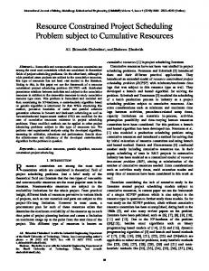
Despite the availability of a plethora of project management software tools (De Wit and Herroelen1, Kolisch2, Maroto et al.3) and extensive research efforts in the area of resource-constrained project scheduling during the past several years (for recent overviews, see Brucker et al.4, Demeulemeester and Herroelen5, Herroelen et al.6, Kolisch and Padman7, Özdamar and Ulusoy8), it is still often the case that projects do not come in on time and on budget. Many reasons for this phenomenon have been described in the literature. The Standish Group surveyed IT executive managers for their opinions about why projects succeed (Standish Group9). The three main reasons why projects are successful were identified as user involvement, executive management support, and a clear statement of requirements. Proper planning ranked as number four. This paper supports the argument that the lack of proper planning is a main source of project failure. Many of the insights provided by the extensive project scheduling research output have not found a place in the decision processes of many practicing project managers, whose scheduling mindset risks being affected by a number of dangerous scheduling misconceptions that still go round within the project management practitioners‟ community and project management periodicals. It is the objective of this paper to identify important potential fallacies and discuss their implications in both deterministic and stochastic project settings. As a vehicle of analysis we will rely on the project shown in Figure 1 in activity-on-thenode format. The project consists of eight real activities, a dummy start activity (activity 1) and a dummy end activity (activity 10). Both dummy activities have zero duration. The planned duration of an activity is shown above the corresponding node. The number shown below each node is the requirement per period (in number of units) for a single renewable resource type. The renewable resource has a constant per period availability of 10 units.
The arcs in the network denote finish-start
precedence relations with zero time-lag, which allow an activity to start as soon as all its immediate predecessors are finished.
Insert Figure 1 about here
4
Critical path versus critical sequence
Hundreds of textbooks and/or textbook chapters have been written on PERT/CPM emphasizing the computation of the so-called critical path as the longest ordered sequence of activities through the project network. In general, commercial project planning software packages allow for a straightforward critical path analysis, which involves, for each activity, the computation of an earliest possible start and finish time (computed respectively as the earliest date an activity can begin (finish), given a project start date and the precedence relations) and a latest allowable start and finish time (computed as the latest date an activity may start (finish), given a project due date and the precedence relations). The total slack (total float) of an activity is then computed as the difference between the activity‟s earliest and latest start times. Each of the activities on a critical path (obviously, there may be more than one such path) is said to be „critical‟ or „slackless‟. To delay one of them would delay the planned completion date of the project. Other activities with positive slack may be delayed up to the amount of their total slack without such an effect, thus giving the scheduler some freedom in assigning start times for each of the activities. We are now ready to introduce a first and fundamental misconception:
Possible Misconception 1: The critical path determines the project duration.
With over 100,000 members worldwide, the Project Management Institute (PMI) is one of the leading non-profit professional associations in the area of project management. Its PMBOK® Guide11 (p. 200) defines the critical path as “the series of activities that determines the duration of the project”. This „critical path‟ notion indeed invites project managers to become trapped in the erroneous belief that the critical path determines the duration of a project, the misconception that the critical path activities are always the ones that require the most attention during planning and that effective project control implies that management should invariably concentrate their control efforts especially on the critical path activities during project execution. As already shown by Wiest12, however, the notion of criticality assumes that (a) activity durations are fixed, and (b) that unlimited resources are available for assignment to the project activities. It has been known among project scheduling
5
scholars for a very long time (e.g. Klingel13), that the deterministic critical path – even in the absence of resource constraints – underestimates the likely project duration when activity durations are uncertain. PERT gives the semblance of accounting for realistic project duration variation in that it calls for three time estimates for each network activity (optimistic, most likely, and pessimistic duration) and by approximating the probability of completing any network event by any given date. However, PERT fails to account for time delays resulting from path interactions. It examines time variances one path at a time and therefore does not account for the probabilities that merging paths may come in late to the path being analysed. The way out provided by Monte Carlo simulation (a) seems to be more difficult to understand and/or apply for project management staff, (b) still neglects the fact that resources are generally limited in availability, and (c) presents the Parkinson‟s Law dilemma (if management understands that the simulated project duration is longer than the deterministic critical path duration, it is tempted to inflate the individual activity time estimates (Schonberger14)). As for the impact of limited resource availabilities, it is well known within the project scheduling research community that (a) slack values depend upon the rules or procedures used for generating and executing the project schedule (see e.g. Bowers15, Raz and Marshall16, Tormos and Lova17), (b) the notion of a critical path loses all meaning (Williams18), and (c) given certain assumptions about project execution, one can identify one or more critical sequences (Wiest12, Woodworth and Shanahan19), each being a chain of activities with zero schedule dependent total slack and composed of precedence and/or resource dependent sub-chains, the length of which determines the deterministic project duration. What the critical chain methodology (Goldratt20) identifies as a critical chain is actually a critical sequence. We can illustrate the issue on the example project of Figure 1. The results of the critical path analysis are shown in Table 1. The path is the longest, hence critical, path with a length of 11 time periods. From a critical path mindset, management should concentrate on the critical path and its constituent activities, because the critical path is assumed to determine the project duration.
Insert Table 1 about here
6
As shown in Figure 2, scheduling the activities as soon as possible, i.e. at their planned early start time, however, yields a schedule that violates the resource availability constraint of 10 resource units per period. Moreover, resource usage is not levelled over the project horizon. We examine the case in which we want to generate a precedence and resource feasible schedule with minimum duration. Stated otherwise, we search for a solution to the well-known resource-constrained project scheduling problem.
Figure 3 shows the resulting minimum duration project
schedule.
Insert Figure 2 about here
Insert Figure 3 about here
By pure luck, the project duration of 11 periods equals the length of the critical path . Also, this critical path is actually one of the 16 different critical sequences that determine the project duration, to wit: , , , , , , , , , , , , , , , and . Every activity in the schedule has zero total slack, whichever choices are made for project execution. The resource profile shown in Figure 3 is perfectly levelled: clearly, the solution is also optimal with respect to the resource levelling problem (generate a levelled schedule that meets the precedence constraints and completes the project within the given deadline of 11 time periods) and allows to identify an optimal solution to the resource investment problem (determine the smallest resource availability that allows the project to be finished by its deadline).
For a thorough discussion of these
problems and a review of solution methods, we refer to Demeulemeester and Herroelen5. It is well known that the three problems for which Figure 3 contains the optimal solution belong to the class of NP-hard problems, so that in real-life project planning it is common practice to rely on heuristic solution procedures.
Most
commercial project planning software packages do not go for the optimum but use priority rule based heuristics to generate resource feasible schedules. Some of them
7
apply a standard built-in procedure (e.g. Microsoft Project) that is often not revealed to the software user, others (e.g. Suretrak and Primavera) provide the user with an extensive list of scheduling (levelling) heuristics to choose from. Using, for example, the earliest start priority rule to generate a feasible schedule for the problem of Figure 1 with constant resource availability of 10 units, in other words applying a serial schedule generation scheme using the priority list L= (1,2,3,4,5,6,7,8,9,10), would generate the resource profile shown in Figure 4.
Insert Figure 4 about here
The schedule of Figure 4 clearly illustrates a second misconception:
Possible Misconception 2: Looking for the best procedure for resolving resource conflicts does not pay off: its impact on the planned project duration is negligible.
As can be seen, the project duration has gone up to 20 time periods, an increase of almost 100%. Actually, quite a number of different activity lists may be constructed that yield a 20-period project duration through the application of a serial schedule generation scheme. The critical path definitely no longer determines the project duration. The project length is now determined by two critical sequences: (in which case activity 4 could be right-shifted over two periods) or (in which case activity 3 could have a two-period right-shift). As can be seen from our analysis so far, the notion of a critical sequence is schedule dependent. The precise procedure used to schedule project activities under resource constraints clearly has an important impact on the resulting project duration and on the critical sequence(s) that determine this makespan. The application of the early start priority rule to our problem example led to a project duration increase of almost 100% above the optimum.
Extensive
computational experiments (Kolisch21) reveal that the late start time rule and late finishing time rule rank among the best priority rules, but still may generate project durations which are more than 5% above the optimum on the average. The problem is that the manuals for most software packages regard scheduling information as proprietary information and, as a result, do not offer a detailed description of the rules
8
in use. Some packages enable the user to select a priority rule from a (sometimes very extensive) list, while others do not. Anyhow, if management relies on commercial software for the generation of a baseline schedule, the result may be far from the optimum (even if only a few activities are involved), especially if resource contention is rather tricky and the “wrong” priority rule is chosen. Computational experiments with seven commercial packages on 160 test instances (Kolisch22) reveal that the average performance is variable, with the best package deviating on the average 4.39% and the worst package deviating on the average 9.76% from the optimum makespan. The mean deviation from the optimum makespan is 5.79%, while the standard deviation calculates to 7.51% and the range is from 0 to 51.85%.
Scheduling under resource constraints and the critical chain
The majority of popular project management textbooks and project planning chapters in operations management textbooks do not dwell deeply on the resource scheduling issue, leaving the impression that it is not that important which method is used to generate a resource-feasible schedule, and thus inviting their readers to adopt Misconception 2. The PMBOK®Guide11 only devotes a 20-line paragraph (p. 76) to resource levelling heuristics, without even recognizing the essential difference between resource levelling (levelling resource use over the project horizon for a given project deadline) and resource-constrained project scheduling (minimizing the project duration subject to the precedence and resource constraints). Some authors even go one step further and actually refute the relevance of project scheduling procedures entirely. In his book describing the critical chain methodology, Goldratt20 (pp. 217-221) argues that project scheduling procedures do not matter because “in each case the impact on the lead time of the project is less than even half the project buffer”.
His critical chain methodology builds a baseline
schedule using aggressive median or average activity duration estimates. Activity due dates and project milestones are eliminated and multi-tasking (more than one activity is performed by the same resource unit at the same time) is to be avoided. In order to minimize work-in-progress (WIP), a precedence feasible schedule is constructed by scheduling activities at their latest start times based on critical path calculations. If resource conflicts occur, they are resolved by “moving activities earlier in time”. The
9
critical chain is then defined as the chain of precedence and resource dependent activities that determines the overall duration of a project. If there is more than one such chain, an arbitrary choice is made. A project buffer (PB), positioned at the end of the critical chain, should protect the project due date promised to the customer from variability in the critical chain activities. Feeding buffers (FB) are inserted whenever a non-critical chain activity joins the critical chain: their aim is to protect the critical chain from disruptions on the activities feeding it, and to allow critical chain activities to start early in case things go well. Although more detailed methods can be used for sizing the buffers (e.g. Newbold23), the default procedure is to use the 50% buffer sizing rule, i.e. to use a project buffer of half the project duration and to set the size of a feeding buffer to half the duration of the longest non-critical chain path leading into it. Resource buffers, usually in the form of an advance warning, are placed whenever a resource has to perform an activity on the critical chain, and the previous critical chain activity is done by a different resource. The critical chain methodology has received a lot of attention in the project management literature and has recently emerged as one of the most popular approaches to project management (Newbold23, Leach24). Internet discussion groups have
been
set
up
to
discuss
the
critical
chain
scheduling
issues
(http://www.apics.org/lists/default.htm; http://groups.yahoo.com/group/criticalchain; http://groups.yahoo.com/group/tocexperts).
Real-world applications by companies
such as Lucent Technologies and Harris Semiconductor have been described to demonstrate the effectiveness of the approach (Leach24, Umble and Umble25). Commercial software has been made available on the market (for example ProChain® (Prochain Solutions, Inc., http://www.prochain.com/index.asp) and cc-Pulse® (Spherical Angle, http://www.sphericalangle.com/).
Critical chain concepts are
promoted as a significant breakthrough in project management. “Indeed, the ideas have been so widely praised and endorsed, and have achieved such impressive results, that one wonders why they have not become the „mainstream‟ of project management” (Yourdon26). Figure 5 shows the buffered schedule obtained using the ProChain software, one of the best known software packages that rely on the critical chain methodology. The software selects the critical chain , and using the 50% buffer sizing rule, generates three so-called feeding buffers: a two-period feeding buffer to protect
10
the project buffer from variation in activity 2, a three-period feeding buffer to protect critical chain activity 9 from variation in the path , and a one-period feeding buffer to protect critical chain activity 8 from variation in activity 5. In addition a sixperiod project buffer is inserted that allows to set the project due date to 20 and to protect it against variation in the critical chain. The resource buffer, inserted in front of activity 7 to give a warning signal to the extra resource unit needed for the execution of critical chain activity 7, is not shown in Figure 5.
Insert Figure 5 about here
The buffered schedule in Figure 5 allows us to reveal a misconception that is widespread among critical chain schedulers:
Possible Misconception 3: During schedule execution, management should closely manage especially the critical chain activities, since it is the critical chain that determines the project duration.
The chain of activities that formed a critical chain in the un-buffered schedule of Figure 3, no longer determines the project duration in the buffered schedule of Figure 5: it now has gaps, i.e. it is no longer the longest contiguous chain of precedence and/or resource-constrained activities whose summed durations determine the length of the schedule. Assume now that management holds on to Misconception 2, selects the 20period schedule of Figure 4 to be used as input to the buffering process, and selects the critical chain . The result will be the buffered schedule shown in Figure 6.
Insert Figure 6 about here
A one-period feeding buffer protects critical chain activity 7 from variation in activity 4 (that suffers a two-period right-shift) and a ten-period project buffer (using the 50% buffer sizing rule) inflates the project due date to 30 periods, a 50% increase. Clearly,
11
steering clear of Misconception 2, in other words relying on a „good‟ scheduling rule and selecting a „good‟ critical chain for buffering, pays off. Both the procedures used to generate the un-buffered schedule and to select a critical chain, have a clear impact on the resulting schedule duration, and hence, on the project due date determined during the application of the critical chain scheduling methodology.
Buffering and schedule robustness
The project scheduling literature largely concentrates on the generation of a precedence and resource feasible schedule that „optimises‟ the scheduling objective(s) (most often the project duration).
During project execution, however, project
activities are subject to considerable uncertainty, which may lead to numerous schedule disruptions. This uncertainty can stem from a number of possible sources: activities may take more or less time than originally estimated, resources may become unavailable, material may arrive behind schedule, ready times and due dates may change, new activities may have to be incorporated or activities may have to be dropped due to changes in the project scope, weather conditions may cause severe delays, etc. A disrupted schedule incurs higher costs due to missed due dates and deadlines, resource idleness, higher work-in-process inventory and increased system nervousness due to frequent rescheduling. In other words: uncertainty lies at the very heart of project management. A schedule that is determined to be optimal with regard to some objective function before its execution may be very vulnerable to minor or serious disruptions. As an illustration, consider the schedule shown in Figure 3, with a perfectly levelled resource profile. This schedule, however, is extremely vulnerable to uncertainty. The slightest delay in the starting time of an activity and/or the slightest increase in the duration of any activity, for example, will lead to an immediate increase in the project makespan. The true optimality of the schedule can only be ascertained in conjunction with its execution in the real world. The proposed schedule, looked upon as „optimal‟ in the project planning phase, clearly has insufficient built-in „slack‟, or flexibility for dealing with unexpected events. In other words, it is not „robust‟. A good approach indeed to account for variation during planning is to build in buffers at strategic points in the project – for instance, increased capacity or budget
12
reserves (De Meyer et al.27). From a scheduling viewpoint, we can cite the common practice of adding “weather delay” to the end of the schedule (so-called “(weather) contingency”, see Clough and Sears28 and O‟Brien29). De Meyer et al. also refer to Cusumano and Selby30 as an example of the fact that time buffers are routinely applied in software projects. It has been the merit of the critical chain scheduling method to cast a number of isolated insights into an integrated project planning and execution approach. There do remain some pitfalls, however. For instance, careful examination of Figure 6 exposes an important misleading assertion about the role and use of feeding buffers in critical chain scheduling:
Possible Misconception 4: The feeding buffers act as a pro-active mechanism to protect the critical chain from distortions in its feeding chains.
The feeding buffer in Figure 6 fails to act as a proactive protective mechanism. A slight disturbance in the duration of activity 4 does not lead to an immediate penetration of the feeding buffer, and so – according to the critical chain buffer management principles – does not generate a buffer penetration alert and hence, does not call for immediate management action. However, it immediately generates a resource conflict with critical chain activity 6, and hence, causes a delay in the critical chain leading to an immediate penetration of the project buffer. More generally, we can conclude that local time buffers will not always be sufficient to protect the project makespan from local disruptions, due to various resource interactions between the project activities. In practice, a project schedule serves very important functions (see Herroelen and Leus31 Mehta and Uzsoy32). The first is to allocate resources to the different activities to optimise some measure of performance. As mentioned by Bowers15, it may be necessary to make advance bookings of key staff or equipment to guarantee their availability, especially in a multi-project environment. The second, as also pointed out by Wu et al.33, is to serve as a basis for planning external activities such as material procurement, preventive maintenance and delivery of orders to external or internal customers. Project schedules are the starting point for communication and coordination with external entities in the company‟s inbound and outbound supply
13
chain. It may for instance be necessary to agree on a time window for work by subcontractors. Based on the baseline schedule, agreements are made with suppliers to deliver materials, support activities are planned (set-ups, supporting personnel), due dates are set for the delivery of project results and when considerable cash outflows or inflows are associated with intermediate activities, cash flow projections will use the baseline schedule for budgeting purposes. A number of these planning purposes were referred to already by Henry Gantt in his writings in the beginning of the twentieth century (cfr. Wilson34). Robust scheduling constructs a schedule while expressly including protection against the manifestation of variability during project execution. The term quality robustness is often used when referring to the insensitivity of the schedule performance in terms of the primary objective value, usually the makespan. Stability or solution robustness refers to the insensitivity of the activity start times to changes in the input data. Willis35 and Li and Willis36 define a stable schedule as “one that does not drastically alter activity start and finish times (...) when the project is rescheduled (...)”.
Indeed, only a stable schedule will allow to exploit the
aforementioned planning purposes to their full extent, in that agreements on future time windows are at all possible. Willis35 makes it seem as if, for initial schedule development, only „poor‟ heuristics (in the sense that they tend to yield higher makespan) should be used, since with these there will always be sufficient spare capacity under the resource constraints to allow increases in activity duration without the need to drastically alter the entire schedule. We reformulate this idea into:
Possible Misconception 5: There is a trade-off between the pre-schedule project duration and solution robustness: the larger the project duration of the baseline schedule, the more stable the schedule.
Insert Figure 7 about here
In terms of solution robustness, the schedule of Figure 7 outperforms the buffered schedules shown in Figures 5 and 6 for disruption scenarios with small (e.g. one period) extensions in the activity durations, in spite of its makespan of only 14 time
14
units. In the schedule of Figure 7, a one-period extension of the duration of any of the activities has no impact at all on the planned starting times of the other activities. In the schedule of Figure 6, an extension of the duration of any activity affects the starting times of its successors in the schedule, while in the schedule of Figure 5, only a one-period increase in the duration of activities 2, 6 or 9, does not lead to a disruption in the start times of the other activities (taking into account the resource usages). In fact, the schedule shown in Figure 7 can be used to illustrate most of the misconceptions that we have discussed so far. The schedule has been generated by means of a „naive‟ protection strategy applied to the minimum makespan schedule of Figure 3, simply by introducing a one period slack between the activity pairs (4,5), (3,7), (6,8), and (2,9). The planned project duration equals 14 time periods, the same duration as obtained for the buffered Prochain schedule of Figure 5 (without the project buffer). The critical path in the project network does not determine the project duration in the schedule of Figure 7 as it contains three one-period gaps. We notice again that an effective procedure for project scheduling under resource constraints clearly pays off. Indeed, the project duration of 14 periods is much smaller than the makespan obtained using, for example, the early start heuristic used to derive the schedule shown in Figure 4. It makes no sense to ask management to concentrate on some “critical chain” during the execution of the project schedule, since the schedule contains three one-period gaps, and so there is no critical chain. Nevertheless, very importantly, in terms of quality robustness the schedule shown in Figure 7 outperforms the schedule of Figure 6 and displays performance comparative with that of Figure 5. With respect to solution robustness, the schedule shown in Figure 7 is better than both schedules shown in Figure 5 and 6. In comparison to the buffered schedule of Figure 6, and keeping the same project due date of 30, the schedule now offers a total protective slack of 16 periods (significantly higher than the length of the project buffer in Figure 6). At the same time, using the same tenperiod protection as offered by the project buffer in the critical chain solution of Figure 6, management can afford to use a much tighter project due date. The due date can now be safely set to 24, a 6-period gain.
15
In generating baseline schedules, one is tempted to use scheduling procedures that generate active or semi-active schedules, because it is well known that for the resource-constrained project scheduling problem there is always an optimal solution that is active (Sprecher et al.37). A schedule is called active if it does not allow for a global left shift of activities; a schedule is called semi-active if it does not allow for activities to be locally left-shifted. The set of active schedules is a subset of the set of semi-active schedules. The schedule shown in Figure 3 is active: no activity can be locally or globally left-shifted. The schedule of Figure 7 is not semi-active, as it allows for local left-shifts. The schedule shown in Figure 8 has been generated by applying a serial schedule scheme using the activity list L=(1,2,3,4,6,5,7,8,9,10). The figure also shows the feeding buffer FB4-7, that would be inserted by the critical chain scheduling procedure, assuming that the chain would be selected as the critical chain, as well as the ten-period project buffer that would be inserted if the 50% buffer sizing rule were used.
Insert Figure 8 about here
The schedule depicted in Figure 8 is clearly active in that it does not allow for local nor global left-shifts. It can immediately be seen that despite its greater makespan, the schedule is not stable: any distortion in the start times or durations of activities leads to a distortion in the start times of all the successor activities in the schedule. This example allows us to elaborate on Possible Misconception 5: there is only a trade-off between pre-schedule project duration and stability if we admit also other than only active schedules. The reason is that in an active schedule, each activity is immediately „dependent‟ on at least one of his predecessor activities in the schedule, because otherwise a left shift would still be possible.
As a result, almost by
definition, active schedules tend to exhibit low solution robustness.
Summary and conclusions
The objective of this paper was to identify and illustrate possible misconceptions that may hamper successful project planning. We have demonstrated that in the presence of resource constraints:
16
the notion of the critical path, defined as the longest path in the project network, loses all meaning;
the procedure chosen to resolve resource conflicts may have an important impact on the planned project duration;
the critical chain identified by applying the critical chain scheduling methodology may not determine the project duration;
time buffers are not always sufficient to isolate local disruptions due to resource interactions;
there is only a trade-off between pre-schedule project duration and stability if we allow for other than active schedules;
active schedules are not necessarily the shortest in duration, nor the most stable.
Acknowledgement This research has been supported by project OT/O3/14 of the Research Fund K.U.Leuven.
17
References 1 De Wit J and Herroelen W (1990). An evaluation of microcomputer-based software packages for project management. Eur J Opl Res 49: 102-139. 2 Kolisch R (1999). Resource allocation capabilities of commercial project management software packages. Interfaces 29: 19-31. 3 Maroto C, Tormos P and Lova A (1998). The evolution of software quality in project scheduling, In Weglarz J (ed.), Project Scheduling – Recent Models, Algorithms and Applications, Chapter 11. Kluwer Academic Publishers: Boston, pp 239-259. 4 Brucker P, Drexl A, Möhring, R, Neumann, K and Pesch, E (1999). Resourceconstrained project scheduling: Notation, classification, models and methods. Eur J Opl Res 112: 3-41. 5 Demeulemeester E and Herroelen W (2002). Project Scheduling – A Research Handbook. International Series in Operations Research and Management Science Vol. 49. Kluwer Academic Publishers: Boston. 6 Herroelen W, De Reyck B. and Demeulemeester E. (1998). Resource-constrained project scheduling – A survey of recent developments. Comp and Opns Res 25: 279-302. 7 Kolisch R and Padman R (2001). An integrated survey of deterministic project scheduling. Omega 49: 249-272. 8 Özdamar L and Ulusoy G (1995). A survey on the resource-constrained project scheduling problem. IIE Trans 27: 574-586. 9 Standish Group (1994). The Chaos Report. The Standish Group International, Inc. (available at http://www.pm2go.com/sample_research/chaos_1994_1.asp accessed 25 September 2003) 10 Wiest JD and Levy FK (1977). A Management Guide to PERT/CPM: with GERT/PDM/CPM and Other Networks. Prentice-Hall, Inc.: Englewood Cliffs 11 Project Management Institute (2000). A Guide to the Project Management Body of Knowledge (PMBOK® Guide). Newton Square. 12 Wiest JD (1964). Some properties of schedules for large projects with limited resources. Ops Res 12: 395-418. 13 Klingel ARJr (1966). Bias in PERT project completion time calculations for a real network. Mgmt Sci 13: B194-B201. 14 Schonberger R (1981). Why projects are always late: a rationale based on manual simulation of a PERT/CPM network. Interfaces 11: 66-70.
18
15 Bowers JA (1995). Criticality in resource constrained networks. J Opl Res Soc 46: 80-91. 16 Raz T and Marshall B (1996). Effect of resource constraints on float calculations in project networks. Int J Proj Mgmt 14: 241-248. 17 Tormos P and Lova (2001). Tools for resource-constrained project scheduling and control: forward and backward slack analysis. J Opl Res Soc 52: 779-788. 18 Williams TM (1992). Criticality in stochastic networks. J Opl Res Soc 43: 353357. 19 Woodworth BM and Shanahan S (1988). Identifying the critical sequence in a resource-constrained project. Int J Proj Mgm 6: 89-96. 20 Goldratt E (1997). Critical Chain. The North River Press Publishing Corporation: Great Barrington. 21 Kolisch R (1995). Project Scheduling under Resource Constraints. PhysicaVerlag: Heidelberg. 22 Kolisch R (1999). Resource allocation capabilities of commercial project management software packages. Interfaces 29: 19-31. 23 Newbold RC (1998). Project Management in the Fast Lane – Applying the Theory of Constraints. The St. Lucie Press: Cambridge. 24 Leach, LP (2000). Critical Chain Project Management. Artech House Professional Development Library: Boston. 25 Umble M and Umble E (2000). Manage your projects for success: An application of the theory of constraints. Prod Inv Mgmnt J 41: 27-32. 26 Yourdon E (2003). Death March, 2nd edition. Prentice Hall, Inc: New Jersey. 27 De Meyer A, Loch CH and Pich MT (2002). Managing project uncertainty: from variation to chaos. MIT Sloan Mgmt Rev Winter: 60-67. 28 Clough RH and Sears GA (1991). Construction project management. John Wiley & Sons Inc.: New York. 29 O‟Brien JJ (1965). CPM in Construction Management: Scheduling by the Critical Path Method. McGraw-Hill. 30 Cusumano MA and Selby MW (1995). Microsoft Secrets. Free Press: New York. 31 Herroelen W and Leus R (2003). Project scheduling under uncertainty – survey and research potentials. Eur J Opl Res: to appear.
19
32 Mehta SV and Uzsoy RM (1998). Predictable scheduling of a job shop subject to breakdowns. IEEE Trans Rob Autom 14: 365-378. 33 Wu SD, Storer HS and Chang P-C (1993). One-machine rescheduling heuristics with efficiency and stability as criteria. Comp and Opns Res 20: 1-14. 34 Wilson JM (2003). Gantt charts: a centenary appreciation. Eur J Opl Res 149: 430-437. 35 Willis RJ (1985). Critical path analysis and resource constrained project scheduling – theory and practice. Eur J Opl Res 21: 149-155. 36 Li RK-Y. and Willis RJ (1993). Resource constrained project scheduling within fixed project durations. J Opl Res Soc 44: 71-80. 37 Sprecher A, Kolisch R and Drexl A (1995). Semi-active, active and non-delay schedules for the resource-constrained project scheduling problem. Eur J Opl Res 80, 94-102.
20
4
2 9 2 0
3 3 2
1 0
4
8 2
7 6 2
5 4
Figure 1
3
6 3
8 7
4
9 2
0
10 1
0
21
resource units
6
5 3
7
4 10
6 2 8 0
Figure 2
1
2
3
4
5
9 6
7
8
9
10
11
time
22
resource units 10
3
5
6
2
7
4
8 0
Figure 3
1
2
3
4
5
9 6
7
8
9
10
11
time
23
resource 10 units
4 2
6 3
0
Figure 4
1
2
3
4
5
7
5 6
7
8 8
9
10
11 12 13
14 15
9 16
17
18 19 20 time
24
2 3
1
6
5
Figure 5
1
FB
FB
4 0
FB
7 2
3
8 4
5
6
9 7
8
9
10
11 12 13
PB 14
15 16
17
10 18 19
20 time
25
resource units 10 FB
4 2
6 3
0
Figure 6
5
7
5 8 10
9 15
PB 20
30
time
26
resource units 10
5
3
6 4
2
7 8
0
Figure 7
5
9 10
15
20
30
time
27
resource units 10 FB 4-7
4 2
6 3
0
Figure 8
5
7 5 8 10
15
9
PB 20
30
time
28
Activity
Duration
Earliest
Earliest
Latest
Latest
Total
start
finish
start
finish
slack
1
0
0
0
0
0
0
2
4
0
4
7
11
7
3
2
0
2
2
4
2
4
2
0
2
0
2
0
5
2
0
2
2
4
2
6
3
2
5
4
7
2
7
2
2
4
2
4
0
8
3
4
7
4
7
0
9
4
7
11
7
11
0
10
0
11
11
11
11
0
Table 1
29
FIGURE CAPTIONS
Figure 1. Project network example (Wiest and Levy10) Figure 2. Earliest start schedule Figure 3. Minimum duration schedule Figure 4. Schedule generated by the earliest start heuristic Figure 5. Buffered schedule generated using Prochain Figure 6. Buffered schedule obtained from the schedule of Figure 4 Figure 7. Naively protected baseline schedule Figure 8. Buffered active schedule
30
TABLE CAPTIONS
Table 1. Critical path analysis