Broken line smoothing for data series interpolation by incorporating an explanatory variable with denser observations: Application to soil-water and rainfall data Nikolaos Malamos1* and Demetris Koutsoyiannis2 1
Department of Agricultural Technology, Technological Educational Institute of Western Greece, Amaliada, Greece 2 Department of Water Resources and Environmental Engineering, School of Civil Engineering, National Technical University of Athens, Zographou, Greece *
[email protected] Abstract Broken line smoothing is a simple technique for smoothing a broken line fit to observational data and provides flexible means for interpolation. Here an extension of this technique is proposed, which can be utilized to perform various interpolation tasks, by incorporating, in an objective manner, an explanatory variable available at a considerably denser dataset than the initial main variable. The technique incorporates smoothing terms with adjustable weights, defined by means of the angles formed by the consecutive segments of two broken lines. The mathematical framework and details of the method as well as practical aspects of its application are presented and discussed. Also, examples using both synthesized and real world (soil water dynamics and hydrological) data are presented to explore and illustrate the methodology. Key words broken line smoothing; interpolation; explanatory variable; GCV; hydraulic conductivity; rainfall
INTRODUCTION
In numerous scientific and engineering applications the dependence of a variable y on another variable x, described by a fitted curve, is exploited for purposes such as interpolation between measurements, prediction, filling in missing values in time series, estimation and removal of the measurement errors, etc. Whenever the mathematical expression of the dependence of y on x is of an a priori known type (e.g. linear, logarithmic, power, polynomial, etc.) the problem of curve fitting is simplified as the only requirement is the determination of the parameters of this expression, a task typically accomplished using regression techniques. The difficulty arises when such an expression is not known and cannot be approximated by a simple easily recognizable formulation. Currently, a lot of methods exist which can accomplish this task using appropriate computer codes and they are mainly used for spatial interpolation in environmental studies. They fall into three categories (Li and Heap 2008): (1) (2)
(3)
Non-geostatistical methods such as: splines (Craven and Wahba 1979 ; Wahba and Wendelberger 1980) and regression methods (Davis 1986); Geostatistical methods including different approaches of kriging, such as: universal kriging, kriging with an external drift or cokriging (Goovaerts, 1997; Burrough and McDonnell 1998); and Combined methods such as: trend surface analysis combined with kriging (Wang et al. 2005) and regression kriging (Hengl et al. 2007).
Koutsoyiannis (2000), introduced the easy method of broken line smoothing (BLS) as a simple alternative to numerical smoothing and interpolating methods, closely related to piecewise linear regression and to smoothing splines. The idea is to approximate a smooth curve that may be drawn for the data points (xi, yi) with a
broken line or open polygon which can be numerically estimated by means of a least squares fitting procedure. The abscissae of the vertices of the broken line do not necessarily coincide with xi’s but they can form a series of points with some chosen, lower or higher, resolution. The main concept of the method is the trade-off between two objectives, i.e. minimizing the fitting error and the roughness of the broken line. The larger the relative weight of the second objective is, the smoother the broken line resulting by the fitting procedure will be. This study is focused in the combination of two broken lines into a piecewise linear regression model with known break points and adjustable weights. The first broken line is fitted to the available data points while the second incorporates, in an objective manner, the influence of an explanatory variable available at a considerable denser dataset. The objective is to make the interpolation across the data points as accurate as possible. The method is illustrated using three applications: a) a theoretical investigational, b) the interpolation of hydraulic conductivity function using water retention data as explanatory variable and vice versa and c) the spatial interpolation of rainfall data using the surface elevation as explanatory variable. METHODOLOGY Mathematical framework
Let (xi, yi) be a set of n points at the x y plane for i = 1,…, n. Let cj, j = 0, …, m, m+1 points of the x-axis so that the interval [c0, cm] contain all xi. For simplicity we will assume that the points are equidistant, i.e. cj – cj–1 = δ and that for every x value we know the value of an explanatory variable t. Therefore, for each point (xi, yi) there corresponds a value t(xi), for i=1, …, n and for a value cj there corresponds a value t(cj), for j=0, …, m. We make the assumption that the dependent variable y in every position x can be expressed as a linear function of the variable t, i.e. y=d+et
(1)
where d and e are coefficients, with their values changing according to x. This is not a global linear relationship but a local linear one as the quantities d and e change with x. Their variation is expressed from two broken piecewise straight lines. At the vertices of the broken lines, the above relationship becomes: yj = dj + ej tj
(2)
We wish to find the m+1 values dj and ej, so that the curve which is defined by the m+1 points (cj, dj + tj ej) and consists of a combination of the two broken lines and of the t(x) curve, ‘fits’ the set of points (xi, yi). This fit is meant in terms of minimizing the total square error among the set of original points (xi, yi) and the fitted curve, i.e. n
p=
(yi – yi)2
(3)
i=1
where yi is the estimate of yi given by the broken lines for the known xi. In matrix form, this can be written as:
p = ||y – y ||2
(4)
where y = [y1,…, yn]T is the vector of known ordinates of the given data points with size n (the exponent T denotes the transpose of a matrix or vector) and y = [y1,…,yn]Τ is the vector of estimates with size n as given by application of equation (1), which for any x can be written as
y(x) = d(x) + t(x) e(x)
(5)
where d(x), e(x) are the ordinates of the corresponding broken lines at point x. Assuming that for some j, cj – 1 ≤ x ≤ cj (see Fig. 1), the ordinate of the broken line d(x) can be determined from: cj – x cj – x d(x) = dj + (dj-1 – dj) c – c = dj + (dj-1 – dj) δ j
(6)
j-1
which can be written as: 1 d(x) = δ [(x – cj-1) dj + (cj – x) dj-1]
(7)
Likewise, the corresponding expression for e is: 1 e(x) = δ [(x – cj-1) ej + (cj – x) ej-1]
(8)
Therefore, if a point xi, lies in the subinterval [cj–1, cj] for some j (1 j m)
then the estimate yi is given by: 1 y^i(xi, t(xi)) = δ {[dj (xi – cj-1) +dj-1 (cj – xi)] + t(xi) [ej (xi – cj-1) + ej-1 (cj – xi)]} (9) If we apply equation (9) for i = 1, 2, …, n, we get : 1 y1 = δ {[d1 (x1–c0)+d0 (c1–x1)]+t(x1) [e1 (x1–c0)+e0 (c1–x1)]}
(10)
1 yn = δ {[dm (xn–cm–1)+dm-1 (cm–xn)]+ t(xn) [em (xn–cm–1)+em-1 (cm–xn)]}
in which we assumed that the point x1 lies in the interval [c0, c1] and point xn lies in the interval [cm–1, cm].
y, d
dj dj-1 d3 d1
yi
d2 d0
x
xi c0
c1
c2
c3
cj-1
cj
Fig. 1: Definition sketch for vector d, adopted from Koutsoyiannis 2000, similar for vector e
The above equations can be more concisely written in the form:
y=Πd+ΤΠe
(11)
[y1,…,yn]Τ
where y = is the vector of estimates with size n; d = [d0,…,dm]T is the vector of the unknown ordinates of the broken line d; e = [e0,…,em]T is the vector of the unknown ordinates of the broken line e; T is a diagonal matrix with its elements: T = diag(t(x1), …, t(xn))
(12)
with t(x1), …, t(xn) being the values of the altitude at the given data points; and Π is a matrix with size n(m+1) whose ijth entry (for i=1, …,n; j=0, …m) is:
xi–cδ j-1, cj-1