the queuing subsystem, which stores these in linked list queues after a ..... S. Iyer, R. R. Kompella, and N. McKeown, âAnalysis of a Memory. Architecture for Fast ...
Buffer Aggregation: Addressing Queuing Subsystem Bottlenecks at High Speeds Sailesh Kumar, Patrick Crowley, Jonathan Turner Department of Computer Science and Engineering Washington University in St. Louis {sailesh, pcrowley, jst} @arl.wustl.edu Abstract — Modern routers and switch fabrics can have hundreds of input and output ports running at up to 10 Gb/s; 40 Gb/s systems are starting to appear. At these rates, the performance of the buffering and queuing subsystem becomes a significant bottleneck. In high performance routers with more than a few queues, packet buffering is typically implemented using DRAM for data storage and a combination of off-chip and on-chip SRAM for storing the linked-list nodes and packet length, and the queue headers, respectively. This paper focuses on the performance bottlenecks associated with the use of offchip SRAM. We show how the combination of implicit buffer pointers and multi-buffer list nodes can dramatically reduce the impact of buffering and queuing subsystem on queuing performance. We also show how combining it with a coarsegrained scheduling can improve the performance of fair queuing algorithms, while also reducing the amount of off-chip memory and bandwidth needed. These techniques can reduce the amount of SRAM needed to hold the list nodes by a factor of 10 at the cost of about 10% wastage of the DRAM space, assuming an aggregation degree of 16.
I.
INTRODUCTION
High speed packet queuing is crucial to the performance of the high throughput packet switching systems used at the core of the Internet. As the Internet takes on a more central role in mission-critical applications, there is a growing need for sophisticated queuing subsystems that can isolate traffic on either a per flow or aggregate flow basis. Such subsystems on router line cards are both a significant contributor to the cost of routers and a potential performance bottleneck because backbone routers require queuing subsystems capable of holding as much data as the link can forward in 100 to 500 ms [1]. An OC192c link translates into queuing subsystems with about 125 to 625 MB of buffer operating at 10 Gb/s rate. With upcoming 40 Gb/s links, both speed and size will quadruple. For routers that implement a simple FIFO output queue, it’s possible to use a very simple queuing architecture in which a large circular buffer is implemented in DRAM. This requires a single on-chip queue descriptor, which provides head and tail pointers and possibly packet and byte counters. One can extend this approach to systems with a small number of queues, but if more than a handful of queues are needed, the static partitioning required by the simple circular buffer leads to significant fragmentation of the memory space. In practice, the circular buffer is difficult to apply even in contexts where the number of separate queues is quite small. The reason for this is that most high throughput routers break variable length packets into smaller fixed length cells for transmission through the switch fabric that connects the line cards together
(we use the term “cell” in a generic sense). This means that cells belonging to different packets arrive at the output side of the router interleaved with one another. The output line card must logically separate them as they come in. One way to do this is to reassemble packets into separate reassembly buffers before passing them to the queuing subsystem. However, this requires a separate buffering stage, which increases memory bandwidth and power consumption. While one might write several packets into the circular buffer concurrently (assuming that the packet lengths are known when the first cell is received), this makes it awkward to discard arriving packets that contain an error that is discovered late in the processing of a packet. For these reasons, the simple circular buffer is rarely used, even in systems where it might seem applicable. Linked lists are a natural alternative to circular buffers. With linked list queues, arriving cells can be stored directly into fixed-size buffers in DRAM; buffer pointers are passed to the queuing subsystem, which stores these in linked list queues after a logical packet reassembly operation has been performed. Linked list queues have the advantage that they place no restriction on how the memory is used. Queues may dynamically share the available memory space or may be restricted in their use, according to policy. This intrinsic flexibility is the key factor in their popularity. However, linked list queues are not without problems. In a typical implementation, queue descriptors are stored in the onchip SRAM, while the linked list nodes themselves are stored in off-chip SRAM. The use of off-chip storage is needed to scale the list node storage in proportion with the DRAM storage. The latency associated with the use of off-chip SRAM can be a serious performance bottleneck. In particular, the rate at which we can perform back-to-back reads from the same queue is limited by the memory latency. While synchronous memory bandwidths have improved significantly in recent years, the memory latency, measured in clock ticks, has been getting worse. This implies that as link speeds continue to increase, the effective worst-case memory bandwidth of the off-chip SRAM will be unable to keep pace. The cost of off-chip SRAM is also a significant concern. While DRAM prices have dropped dramatically over the years, high performance SRAM has remained relatively expensive. On a per byte basis, SRAM is more than 100 times costlier than DRAM. So, in a system that stores a single four byte pointer for every 64 byte memory buffer, the cost of the SRAM can be six times the cost of the DRAM. Increasing the DRAM buffer size provides only a limited relief from this problem, as minimum size IP packets with just 40 bytes are extremely common in Internet traffic.
Another factor crucial to the effectiveness of queuing is the algorithms used to schedule the queues. Practical algorithms can be broadly classified as either timestamp or round-robin. Time stamp based algorithms try to emulate a GPS [2] by sending packets, approximately, in the same order as sent by a reference GPS server. It involves computation of timestamps for various queues, and sorting them in an increasing order. Round-robin schedulers avoid the sorting bottleneck by assigning time slots to the queues and transmitting multiple packets with cumulative size up to a maximum sized packet from the queue in the current slot. Both flavors of these schedulers require retrieving the length of subsequent packets in the queue after transmitting any packet and before scheduling the next packet. Therefore queuing subsystems typically stores the packet lengths in off-chip SRAM along with the linked-list pointers, which ensures faster access while also preserving the scaling of queuing subsystem in proportion to the DRAM. Nevertheless, an off-chip access involved in retrieving the packet lengths remains a potential bottleneck. Several authors [3][4][5] have studied the performance issues surrounding the DRAM used for packet storage, however, relatively little attention have been given to the offchip SRAM. We find that off-chip SRAM can be a significant contributor to the cost of the packet queuing subsystem and can place serious limits on its performance, particularly as link speeds scale beyond 10 Gb/s. This paper shows how queuing subsystems using a combination of implicit buffer pointers, multi-buffer list nodes and coarse grained scheduling can dramatically improve the worst-case performance, while also reducing the SRAM bandwidth and capacity needed to achieve high performance. The remainder of the paper is organized as follows. Details of a linked-list based queuing subsystem are given in section 2. Section 3 introduces buffer aggregation and section 4 analyzes its performance. Section 5 reports the performance results on an experimental queuing setup and section 5 and 6 concludes the paper. II. LINKED-LIST QUEUES AND BOTTLENECKS In this paper, we consider a high performance queuing subsystem architecture using a combination of DRAM for packet storage, on-chip SRAM for queue descriptors and offchip SRAM to implement linked list queues. Linked list queues can be implemented in either of the following two ways: a) implicit mapping in which the address of the linked list nodes in SRAM directly imply the address of the buffers in DRAM, or b) explicit mapping in which buffers are dynamically mapped to the list nodes (consequently the list node explicitly stores the buffer address). Implicit mapping clearly eliminates the need to store buffer identifiers at the nodes. Explicit mapping, on the other hand, is effective for multicasting, because it allows a buffer to exist at multiple list nodes. In this paper, we focus on implicit mapping and leave our multicast solution to future work. The schematic of the queuing subsystem with implicitly mapped linked-list nodes is shown in Figure 1. We enumerate the key features below: DRAM consists of fixed sized buffers; address of each buffer is referred to as the buffer identifier (buffer ID). A free queue keeps all unused buffers. Packet queues hold the active buffers (the stored packets). A buffer is taken from the free queue upon cell (we assume that packets
On-chip 0 11 40B 9 4
SRAM 2
DRAM
96B 1
pkt1, cell1 (40B)
80B 7
Head node T ail node
X
pkt2, cell1(64B)
One-to-one implicit mapping
Head packet length
pkt2, cell2 (32B)
11 40B 1
Free queue descriptor Head Tail
4
X
pkt2, cell1 (16B)
Next node Next SOP bit Next packet length
pkt1, cell1 (64B)
pkt3, cell1 (40B)
Figure 1: Queue structure with implicit mapping; on-chip memory stores queue descriptor, SRAM implements linkedlists and also stores packet lengths, DRAM stores packet data
either arrive as fixed sized cells, or are fragmented as they arrive) arrival and added to the target packet queue. Every linked-list node stores a) the address of the next node of the queue, b) a bit to indicate if a new packet starts at the next node and c) the length of the packet starting at the next node. Storing packet lengths at the node before the one where it starts, saves the write and read associated with the store and retrieve of the packet length, as it is done with the reads and writes of the links. Queues are identified by queue descriptor, which stores the head and tail node of the linked-list. It also stores the length of the first packet in the queue as a consequence of the above feature, where packet lengths are stored one node ahead, which also enables the length of packets at the head of every queue to be readily available (as queue descriptors are kept on-chip). Such a queuing structure provides several benefits: reduced memory fragmentation, few restrictions on queue sizes, and scalability. However, to demonstrate its effectiveness we must consider the following bottlenecks as well. A. Dequeue throughput determined SRAM latency Since linked-list nodes are stored in off-chip SRAM, every dequeue involves an off-chip read access, which is 20 ns even with today’s state-of-the-art technology (considering interchip communication latencies). Thus, whenever multiple cells are sent from a queue, each subsequent cell requires 20 ns, which translates into a throughput of about 25 Gbps with 64byte cells. This is a serious concern since sending multiple cells back-to-back from a singe queue is the common case, considering that average Internet packet length is more than 200 bytes. Moreover, round-robin fair queuing algorithms often send several cells (i.e., the number of cells equaling the maximum packet size) whenever a queue is selected. B. Fair queuing algorithms performance Another potential bottleneck in queuing subsystems is the efficiency of the fair queuing algorithms which schedule the queues. Most queuing algorithms select queues based upon the length of the packet at the head of either the current queue or all queues. When packet lengths are stored in an SRAM (with linked-list nodes in this case), an off-chip reference is required after sending every packet. Pre-fetching the lengths of a few
packets at the beginning of every queue provides only a limited relief, because several packets are sent from a queue, one after another, quite frequently. C. Linked-list memory size, cost and bandwidth A large packet buffer requires a proportionally large memory to store the linked-list nodes. For example, a 512 MB packet buffer requires 40 MB of linked-list memory, approximately 8% of the buffer. Since the per bit cost of SRAM is 100 times higher than DRAM, the cost of this SRAM would be 8 times that of DRAM. Moreover, SRAM of this size requires at least 12 chips (maximum available SRAM density is 36 Mbit per chip) while data memory requires only 4 chips (maximum DRAM density is 1 Gbit per chip). Requiring 16 chips for the packet buffer at every line card clearly raises concerns over the scalability and reliability of the entire system, given the power consumption and on-board design complexity involved. Another issue surrounding such a linked-list structure is the required memory bandwidth. Each arriving and departing packet requires two linked-list operations, one targeting the free queue and one target the destination queue, for a total of 4 operations per arrival/departure time. The fastest commercially available memory (QDR-SRAM running at 250 MHz DDR clock) allows only 4 random accesses every 16 ns while the inter arrival time of 64-byte cells at 40 Gbps is 12 ns. Thus, the random access bandwidth of the linked-list memory is also a potential bottleneck. III. USING MULTI BUFFER LIST NODES We propose using multi-buffer list nodes (also called aggregated buffers) in which every list node contains multiple buffers. Figure 2 illustrates a queue of multi-buffer nodes. When multiple cells are referenced in each linked list node, fewer link list traversals will be required thus reducing the memory bandwidth requirement. Moreover, implicitly mapped multi-buffer nodes reduce the ratio of list nodes to DRAM buffers, thereby reducing the linked-list memory size for a given number of buffers. While memory size is important, the most notable benefit of buffer aggregation is that it ensures that linked-list memory access latency and bandwidth doesn’t limit the performance. Multi-buffer list nodes remains effective for both explicit as well as implicit mapping, however, in this paper, we consider implicit mapping. Implicit mapping, by definition, keeps a one-to-one static map between buffers and list nodes. With buffer aggregation, every list node is uniquely mapped to X buffers where X is referred to as the degree of aggregation. While it is possible to map any arbitrary set of X buffers, such a mapping will unnecessarily complicate the translation of list nodes to buffer IDs. A simple and efficient mapping is direct mapping, in which a set of contiguous buffers are mapped to a list node with the address of the first buffer being the same as the node’s address. A special case occurs when the degree of aggregation is a power of 2, when translation from list node to its buffers involves only bit shifts. We consider such direct one-to-one mappings due to their simplicity and efficiency. A new list node is allocated for an arriving cell only if all X buffers at the tail node of the corresponding queue are full. Similarly, the head node is de-allocated only after transmitting all X buffers from it. Thus, in order to make the node
Queue descriptor Head occupancy
Tail occupancy
Head node
Tail node
Next node
Next node
Next node
...
Next node
Implicit mapping 0 : :
No Data
Cell
Cell
:
:
:
First Cell
:
:
Cell
...
: Last Cell No Data
X-1
:
Figure 2: Queue descriptors, linked list nodes and DRAM buffers (where cells are stored) with buffer aggregation
allocation or de-allocation decision for any cell, the buffer occupancy of the tail and head nodes must be examined. For arriving cells, therefore, the destination queue must be known before the cell can be stored. This means that packet classification must occur prior to storage. It may be argued that this will require additional on-chip buffers to hold the arriving packets while they are classified. We find that this additional buffering is very small in practical systems given that the packet header arrives first and that classification must be fast enough to handle back-to-back minimum sized packets. IV. QUEUING PERFORMANCE WITH BUFFER AGGREGATION When queues are backlogged, aggregated buffers help because, on average, linked list operations and buffer allocations are only required every X cells for aggregation degree X. To demonstrate the broad benefit of aggregated buffers, we must consider two important cases. First, when queues are not heavily backlogged and the average queue length remains low, node allocation and de-allocation may occur more frequently. Second, it may be that many or all queues have a near-empty aggregated buffer at the head position (or a near-full buffer at the tail); in this scenario, a potentially long sequence of de-allocations (and allocations) Before considering these scenarios, we will establish the following result. Lemma 1. Without aggregation, linked-list memory must allow 2 accesses during every T, where T is smaller of the inter-cell arrival and inter-cell departure time. Proof: Let the cell arrival and departure intervals are Ta and Td respectively. For every arriving cell, a node is de-allocated from the free queue and linked to the packet’s queue. Similarly for every departing cell, a node is de-allocated from the packet’s queue and linked to the free queue. While, each of these requires two accesses to the link memory, node reuse (via a free node buffer) can save two accesses during every max(Ta, Td). Therefore during any period max(Ta, Td), we need 2*max(Ta, Td)/min(Ta, Td) accesses. Thus, 2 link accesses during every min(Ta, Td) is sufficient (although a small buffer may be needed to hold few link nodes because the node addition and removal times may be different). ■ A. Scenario 1: when queues remain near empty When average queue length is small, link memory might be accessed relatively frequently, especially if the queue length falls below X cells. If the average queue length is l cells (l < X), a cell will require a link access every l cells. It can be
Linked list memory
1 Ta
1 Ts
1 XTa
Arrival process
enqueuer queue Se
enque uer
Consumes
deque uer
balan cer
Elastic buffer holds free nodes
output queue
Sd = 1 Produces
1 XTs
Departure process (Scheduler)
X-1 XTs
1 Td
So
1 Ts
Figure 3: Queuing subsystem model around the linked-list memory accesses
argued that when l becomes 1, an aggregated buffer will require as many link accesses as in the non-aggregated case resulting in no performance improvement. This is true, however this scenario does not represent a bad case since no link list operations are required (i.e., with only one cell per queue, no back-to-back dequeues will be performed). Rather, aggregated buffers are needed to improve performance under more difficult conditions. B. Scenario 2: backlogged queues with near-empty heads In this scenario, it can be argued that even if linked-list is accessed once for every X cells on an average, the worst-case queuing throughput can remain the same. For example, it is possible that head node of several queues contains only one cell, and these queues are scheduled one after another. Consequently, linked-list will be accessed for every cell and in worst-case it can prevail for as much time as there are queues. Similarly, it is likely that a stream of packets arrive at the queues whose tail node is full. In these worst-case scenarios, linked list accesses can remain quite the same as in nonaggregated case. Moreover, it can also be argued that buffer aggregation might make node reuse1 tricky because their allocation and de-allocation becomes non-deterministic. The arguments for the worst-case scenarios are valid, but we find that adding small enqueue and dequeue buffers to accommodate periods of worst-case node occupancy is an effective way to keep the average performance very high. An importance consequence of this change, however, is that we meet worst-case performance requirements probabilistically. Fortunately, we can show that modest buffering requirements can provide acceptably low drop probabilities. Figure 3 shows our system model. The enqueuer, balancer, and dequeuer nodes represent the active components, which accesses the link memory. The elastic buffer implements node reuse so that deallocated nodes can immediately be allocated to another queue without an off-chip transaction. The input queue at the enqueuer and the output queue at the dequeuer provide buffering during worst-case conditions. The objective is to keep the enqueuer queue near empty and the output queue near full because the probability that enqueuerqueue overflows will be the cell discard probability and the probability that output-queue underflows will be the output link under-utilization. To demonstrate that the system can meet worst-case conditions with very high probability, we 1
When cells arrive and leave at equal rate, list nodes that get freed up can be reused for the arriving cells, thus avoiding memory accesses needed for the free linked-list processing.
have a developed a discrete time Markov model to determine the size distribution of these queues. Comprehensive model details can be found in the Appendix. In the next section, we report the results for an experimental setup and technological parameters. 1. Experimental setup and results In order to validate the effectiveness of buffer aggregation, we will now apply our model to an experimental setup shown in Figure 4. Each link operates at OC768 rate and queuing subsystems are employed at both input and output side of the switch. We assume 64 byte cell switching and consider switch speedups of 1 and 2. With speedup 1, a 40 Gb/s link rate requires one dequeue and one enqueue every 12 ns. With a speedup of 2, the input subsystem has to perform a dequeue every 6 ns (Td), while the output subsystem has to perform an enqueue every 12 ns (Ta). We keep on-chip processing time for enqueues and dequeues (Ts) at 3 ns; thus the on-chip processing speed is sufficient to keep up with the enqueue and dequeue rates. Input Queuing
Output Queuing
:
:
: :
: :
:
crossbar speedup = 1, 2
:
Figure 4: Experimental setup for the queuing subsystem performance analysis; every link rate is OC768 (40 Gbps). Two scenarios with switch speedup 1 and 2 have been considered.
If a next generation QDR-III SRAM running at 333 MHz is used to implement the linked list, it will support a random access every 3 ns (Tm) and will have an access latency of 15 ns (Tr), (assuming an aggressive chip-to-chip communication latency). Memory bandwidth is clearly sufficient (from Lemma 1) even without buffer aggregation. However, access latency clearly exceeds the dequeue intervals of 12 ns and 6 ns, thus cells can’t be dequeued sufficient rates. Buffer aggregation of degree 2 should solve this instance of problem. However, in order to demonstrate the effectiveness of buffer aggregation, we consider a slower SDR-SRAM with a clock period, Tm of 12 ns and latency, Tr of 24 ns. Below, we summarize the performance of aggregated buffers for the different combination of queuing subsystems and speedup.
1E+00
Input queuing, switch speedup = 2
Output queuing, switch speedup = 2
Both queuing, switch speedup = 1
1E-01 1E-02 1E-03 1E-04 Cell loss rate (enqueuer Q = 16) Output link idle (output Q = 32) Cell loss rate (enqueuer Q = 32) Output link idle (output Q = 64)
1E-05 1E-06 2
4
6
8
10
12
14
16
2
4
Degree of aggregation, X
6
8
10
12
14
16
2
4
Degree of aggregation, X
6
8
10
12
14
16
Degree of aggregation, X
1E+00 1E-01 1E-02 1E-03
Enqueuer queue
1E-04
Output queue
1E-05
Degree of aggregation = 12 Input queuing, speedup = 2
1E-06
Degree of aggregation = 8 Output queuing, speedup = 2
Degree of aggregation = 6 Both queuing, speedup = 1
1E-07 0
4
8
12
16
20
24
28
32
0
4
8
Occupancy level
12
16
20
24
28
32
0
4
8
Occupancy level
12
16
20
24
28
32
Occupancy level
Figure 5: A) Upper row plots the cell discard rate and output link utilization for 2 sets of enqueuer queue and output queue sizes). Link rate is 40 Gbps and linked-lists memory clock period is 12 ns and access latency is 24 ns. B) Steady-state probability of the enqueuer queue, and output queues (various queue capacities: output queue = 32, elastic buffer = 16, enqueuer queue = 16).
a) Input/Output queuing; Switch speedup = 1 In this case Ta and Td are both 12 ns. From the analysis presented in the Appendix, queuing subsystems becomes stable with a degree of aggregation of 4 or higher. From the results plotted in Figure 5, it is clear that when degree of aggregation is more than 4, cell discard probability and output link utilization improves with increasing enqueuer/output queues. In the same figure, we also report the steady-state of various states of the enqueuer and output queue. It is apparent that likelihood of the enqueuer queue being full and the output queue being empty is very low. b) Output queuing; Switch speedup = 2 Ta and Td are 6 and 12 ns. Queuing subsystem becomes stable with a degree of aggregation of 4 or higher. We report the above results in Figure 5. c) Input queuing; Switch speedup = 2 Ta is 12 ns and Td is 6 ns. Queuing subsystem becomes stable with a degree of aggregation of 10 or higher and we report the above results in Figure 5. It is apparent from these results that a higher degree of aggregation improves the performance for relatively smaller request buffers. It is also apparent that larger elastic buffer and enqueuer and output queues benefits only when queuing subsystem parameters are stable. V. PACKET SIZE AND COARSE-GRAINED SCHEDULING We have mentioned that most queuing subsystems store packet lengths and boundary bits with the linked-list nodes. Such a structure results in poor space efficiency because a) short packets don’t use all length bits and b) long packets don’t use length bits at the nodes pointing to the middle of packet (MOP). Buffer aggregation can improve this inherent
inefficiency with the help of the following mechanism to encode the packet boundary and length. A. Storing packet boundary and length We use an alternate mark inversion (AMI) encoding to mark the packet boundary, and keep X bits every node for this purpose. A sequence of bits of the same polarity indicates the continuation of a packet. As soon as a bit alternates, the end of the current packet is inferred. To store the packet lengths, we argue that (X-1)log2C+log2P bits at every node is sufficient, where C is the cell size and P the maximum packet size. We take the three possible scenarios and show that these many bits are sufficient. A) When all packets at a node are single cell, they will need a total of X*log2C bits, less than what we have. B) If a packet spans n buffers but lies entirely within a node, it will need log2(n*C) bits while n*log2C bits is available for it, which is sufficient because log 2 (nC ) ≤ n × log 2 C ∀ n > 0 . C) When a packet starts at a node and ends at another, it will need log2P bits. Since, only one such packet can exist at a node, its length can again be stored. The resulting node structure with the boundary and length bits highlighted is shown in Figure 6. Packet length mask Unused
log2C
4*log2C bits Length
log2C
Length Length
log2P bits Length
Packet boundary mask 1
1
0
0
0
0
1
0
1
1
MOP Cell
EOP Cell
SOP/ EOP
SOP/ EOP
SOP Cell
MOP Cell
Data in the buffers at this list node MOP Cell
EOP Cell
SOP Cell
MOP Cell
Figure 6: Data structure to store the packet boundary and length at any list node with a degree of aggregation of 10.
This scheme improves the space efficiency to store packet lengths from log2P bits per cell to roughly log2C bits per cell for higher degree of aggregations. The flip side of a high aggregation is that it increases the size of queue descriptors, which might have to store the packet length and boundary of the head (and possibly the tail) node. We introduce a coarsegrained approach to store the packet lengths, which reduces the queue descriptor size as well as the node sizes. B. Storing packet lengths – a coarse grained approach In this coarse grained approach, we use a clever encoding to store the packet lengths. A multi-buffer node stores only the AMI encoded packet boundary mask (requires X bits) and the cumulative length of all packets starting at the node i.e. whose SOP cell resides there (requires log2(X*C+P) bits). This scheme clearly reduces the space required to store the packet lengths from roughly log2C bits per cell in the first scheme to roughly (log2X*C)/X bits per cell. Consequently, the size of queue descriptor also gets reduced. However, the length of packets (in bytes) beginning at any node can’t be determined with this scheme, therefore the question arises: how will the scheduler schedule the packets? We show that the information present at the nodes is sufficient to ensure a fairly accurate scheduling because the cell count of any packet can be determined. Also, after sending the last packet from a multi-buffer node, the total number of bytes sent from the node can be determined. We will now briefly discuss how fair scheduling can be maintained. C. Using coarse-grained scheduling In coarse-grained scheduling, packet lengths are represented as multiples of cells (64-byte, etc) instead of bytes, and the fair queuing algorithm selects queues based upon cell counts. Note that such a policy might result in persistent unfairness and poor delay bounds for the flows with relatively odd sized packets. For example, in a system with 64-byte cells, a flow with all 65-byte packets will send as many packets as a flow with equal priority and 128-byte packets. In order to ensure long-term fairness, we propose a simple technique which uses the cumulative packet length information stored at every node. With cumulative byte and cell counts of every packet starting at a node known, we compute the normalized average number of bytes in every packet using the following equation, Length (cells) × ∑all packets at node Length (bytes) Length (bytes) = ∑all packets at node Length (cells) When the fair queuing algorithm makes selections based upon the above packet length, long term fairness is ensured. In fact, fairness is ensured within a time window equal to the time needed to send all packets in a single multi-buffer node. Since a maximum of X packets can begin at a node, fairness is ensured for every X packets transmitted from a queue. We leave the further analysis of this issue to future work. VI. SUMMARIZING THE BENEFITS AND DRAWBACKS OF BUFFER AGGREGATION With buffer aggregation, cells can be sent at a rate of X cells per linked-list memory access time, if linked-list accesses are the only bottleneck. A high degree of aggregation will eliminate the bottleneck of linked-list memory access latency
and bandwidth. Indeed, cheaper linked-list memories with less random access bandwidth and higher latencies can be used, as compared to a traditional approach. Another notable benefit of buffer aggregation is a factor of X reduction in the number of linked-list nodes. With the addition of coarse-grained scheduling, this translates into a factor of X reduction in linked-list memory. A large X, therefore, can enable on-chip memories to be used, which will eliminate an external component and the associated interface. However, aggregated buffers may result in wastage of DRAM space when the head and tail nodes are not fully occupied. In the worst case, every queue can waste (X-1) buffers in the head and tail node, thus, Wasted space = 2 × No of queues × ( X − 1) For a system with 512 MB of DRAM, 64 thousand queues, and 64-byte cells; a degree of aggregation of 8 will translate into wastage of about 10% of DRAM space in the worst-case and about 5% in average case. Buffer aggregation might also require a careful design to ensure good DRAM efficiency. With buffer aggregation, arriving cells typically occupy the first available buffer at the tail node. Therefore, traditional DRAM bank arbitration techniques can’t always be used with writes; this can result in reduced DRAM efficiency. We believe that out-of-order writes, along with re-ordering, can solve this problem. Nonetheless, we leave this issue to future work. VII.
CONCLUSIONS
In this paper, we have pointed out the potential bottlenecks associated with the linked-list queuing subsystems as the link rates scales beyond 10 Gb/s. We have proposed the use of buffer aggregation, which employs multi-buffer linked-list nodes. With the aid of a discrete time Markov analysis, we have shown that multi-buffer list nodes can significantly improve queuing throughput and practically eliminate the queuing bottlenecks associated with the linked-list memory bandwidth and access latency. Multi-buffer list nodes when combined with the implicit mapping and coarse-grained scheduling can reduce the amount of SRAM needed to hold the list nodes by a factor of 10 at the cost of about 10% wastage of the DRAM space, assuming an aggregation degree of 16. Such reductions in SRAM size can translate into significant cost savings considering that cost of SRAM frequently dominates that of DRAM in high speed queuing subsystems. REFERENCES [1] [2] [3] [4] [5]
C. Villamizar and C. Song, “High Performance TCP in ANSNET,” Computer Communication Review, Vol. 24, No. 5, pp. 45-60, Oct. 1994. A. K. Parekh, “A generalized processor sharing approach to flow control in integrated services networks,” Ph.D. thesis, Dept. of Elect. Eng. and Comput. Sci., M.I.T., Feb. 1992. S. Iyer, R. R. Compella, and N. McKeown, “Designing Buffers for Router Line Cards,” Stanford University HPNG Technical Report TR02-HPNG-031001, Stanford, CA, 2002. S. Iyer, R. R. Kompella, and N. McKeown, “Analysis of a Memory Architecture for Fast Packet Buffers,” IEEE HPSR’02, Dallas, May 2001. A. Nikologiannis, M. Katevenis, “Efficient Per-Flow Queuing in DRAM at OC-192 Line Rate using Out-of-Order Execution Techniques,” Proc. IEEE Int. Conf. on Communications (ICC'2001), Helsinki, Finland, pp. 2048-2052, June 2001.
APPENDIX Model of the queuing subsystem with bottleneck formulated around the linked list memory bandwidth and access latency is shown in Figure 3 (Section IV). We assume that latency associated with the dequeues from free queue aren’t the bottleneck (multiple free queues can be employed for this purpose and free nodes can be dequeued from them in a round-robin order). We first isolate the arrival and departure processes. Arrival process maps the arriving cells to a queue and enqueues them as quickly as possible. Departure process dequeue cells from the queues selected by the scheduler at a rate sufficient to keep the output link busy. With buffer aggregation, the occupancies of head and tail node increases linearly with arriving cells, thus the occupancy of head and tail node remains random at any random time instant. Therefore, likelihood of nodes allocation and de-allocation remains uniform random with a probability of 1/X, irrespective of the queue selection order. Since linked-list memory is the bottleneck, cells that don’t need a link access are processed quickly while others wait for the memory. We keep a queue at the arrival process to hold such cells and refer to it as enqueue-queue; cells from this queue are processed by an enqueuer as it gets to access the link memory. A similar queue for dequeues can’t be employed because 1) Dequeues has to be performed strictly in order and therefore departure process can’t continue if some requests are waiting for the link access, 2) Even if we allow out-of-order dequeues; due to the linked-list structure, subsequent cells from a queue can be dequeued only after the one requiring the link access is dequeued. 3) Third reason has to do with the operation of scheduler which requires the packet lengths in order to make selections. Since the queuing subsystems, we consider, stores packet length at the list nodes, whenever a dequeue requires link access, length of the next packet is available only after the access is serviced and only thereafter, scheduler can proceed. Our principle metric of the efficiency of departure process is output link utilization, i.e. how often the output link remains busy. We maximize this metric by keeping an output queue in which departure process stores the dequeued cells. This queue is serviced at the output link rate and the objective is to keep it non-empty. In order to simplify the model, we also keep a dequeue-queue. Departure process dequeues the cells right away if link access is not required otherwise puts the request into the dequeue-queue. A dequeuer services the requests from this queue as the link memory is available and puts the dequeued cells in the output queue. Clearly, departure process stalls whenever dequeue-queue remains non-empty, therefore, we keep the size of dequeue-queue at 1. The queuing subsystem also incorporates an elastic buffer, which holds few free list nodes. Enqueuer services requests from the enqueue-queue only if elastic buffer has free nodes available and the dequeuer services requests from the dequeue-queue only if elastic buffer has some free space. A balancing process tries to keep this elastic buffer nearly half filled, by accessing the link memory. Our objective is to compute the probability that the enqueue-queue overflows, which will be the cell discard probability and the probability that output-queue underflows.
We solve the queuing subsystem model (shown in Section IV) using a discrete time Markov analysis. Let Ta and Td be the inter cell arrival and departure times; the linked-list memory allows an access every Tm, with the read access latency being Tr. Also, let the enqueue and dequeue process takes Ts time to service requests that doesn’t need a link access. Thus, the one which needs a link access will take (Ts+Tw) and (Ts+Tw+Tr) respectively, where Tw is the waiting time of a request in the queue. The queuing subsystem is called to be in a stable state when following three conditions are satisfied, X × min(Ta , Td ) (1) Tm < 2 max(Tm + Tr , Ts ) Ts ( X − 1) (2) Td > + X X max(Tm , Ts ) Ts ( X − 1) (3) Ta > + X X Equation 1 requires at most X times lower link bandwidth than in a non-aggregated system given by Lemma 1. Equation 2 requires that the memory latency should have a toll on only one cell among X cells. Equation 3 is similar with the exception that enqueue process doesn’t incur any link read access latency. An ideal queuing subsystem in a stable state, should keep the outgoing link busy and also keep up with the incoming link. With the aid of discrete time Markov analysis, we will now show that an aggregated queuing subsystem, in stable state, also ensures nearly zero cell loss probability and 100% output link utilization. We let the size of enqueue-queue, dequeue-queue, outputqueue and elastic buffer be Se, Sd, So and B, respectively, and fe, fd, fo and f be their fill levels. Note that Sd is 1. In order to enable stable balancing of the elastic buffer, we define a threshold ∆, such that the balancer contends for link access to balance the elastic buffer only when its occupancy deviates by more than ∆ from the mean B/2. We also dynamically give the link access to either enqueuer, or dequeuer or the elastic buffer based on their urgency αe, αd and αb. Urgency is defined as the normalized imbalance and is given by the following equations for the enqueuer, dequeuer and elastic buffer, respectively, α e = fe / Se (4) α d = ( S o − Fo ) / S o (5) ( B / 2 − ∆ − f ) /( B / 2 − ∆ ) when ( B / 2 − ∆ > f ) α b = ( f − B / 2 − ∆ ) /( B / 2 − ∆ ) when ( f > B / 2 + ∆ ) (6) 0 else Clearly, the system performance is maximized when a) the enqueue-queue is least likely to get filled, b) elastic buffer remains balanced and c) output-queue remains non-empty. We will now define a discrete time Markov chain to model the system. We first define a variable t, which increments every unit time and rolls over once it reaches N, where N is the least common multiple (LCM) of Ta, Td, Ts and Tm. t is used as the reference for all events as follows. Probability that a request arrives in the enqueue-queue is, 1 / X when ( f e < S e and t mod Ta = 0) Pe = (7) 0 else Probability that a request arrives in the dequeue-queue is, 1 / X when ( fd = 0 and fo ≠ So and t mod Ts = 0) Pd = (8) 0 else
Probability that a request which doesn’t need a link access, arrives in the output queue is, X −1 when ( fd = 0 and fo ≠ So and t mod Ts = 0) X Po = (9) 0 else Link memory request is serviced whenever (t mod Tm) is 0. We define another variable, w, which indicates the time for which dequeuer must wait to receive the data read from the link memory. w is set to Tr whenever link memory serves the dequeuer, and decrements every unit time thereafter. When it reaches 1, data is received, request from the dequeue-queue is flushed and dequeued cell is written into the output queue. State of the queuing subsystem is defined as (fe, fd, fo, f, w, t). We let π( fe, fd, fo, f, w, t) denote the steady-state probability that the system is in state (fe, fd, fo, f, w, t). To compute the steady-state probabilities of all states, we need to specify transition probabilities that give the probability of a transition from one state to another. Let δ(s1,s2) denote the transition probability from state s1 to state s2. Then, we can write, π ( s 2 ) = ∑s π ( s1 )δ ( s1 , s 2 ) (10) 1 To simplify the specification of the transition probabilities, we view the transition as happening in four phases; an arrival phase followed two service phases, followed by a departure phase. During the arrival phase, new entries may (or may not) arrive in the enqueue, dequeue or output queues. During the first service phase, a memory request from one of the three requesters is serviced. During the second service phase, data read from the link memory may arrive hence the dequeued cell is written into the output queue and the dequeue-request is flushed from the dequeue-queue. During the departure phase, an entry from the output queue is sent. t is incremented and w is decremented during the departure phase. If we let δa(s1,s2), δs1(s1,s2), δs2(s1,s2) and δd(s1,s2) represent the probability of a transition between the phases, and πa(s), πs1(s), and πs2(s) be the intermediate state probabilities, they can be related through the following equations, π a ( s 2 ) = ∑ s π ( s1 )δ a ( s1 , s 2 ) (11) 1
π s1 ( s 2 ) = ∑ s π a ( s1 )δ s1 ( s1 , s 2 ) 1
π s 2 ( s 2 ) = ∑ s π s1 ( s1 )δ s 2 ( s1 , s 2 ) 1
π ( s 2 ) = ∑ s π s 2 ( s1 )δ d ( s1 , s 2 )
(12) (13)
(14) We can use these equations to solve for the steady state probabilities as follows. First, we assign initial values to π(s). To ensure that the system is equally likely to be with any value of t, not just in the steady state, we assume that the reference counter is initialized to a random value. We also let the elastic buffer half filled and other queues empty initially. We reflect these initial values in our model, by initializing π (0,0,0, B / 2,0, t ) = 1 / N for all values of t and letting all the other state probabilities be zero. We use these initial state probabilities, together with the transition probabilities δa(s1,s2) to compute values of πa(s). We then use a) πa(s) and δs1(s1,s2) to compute πs1(s), b) πs1(s) and δs2(s1,s2) to compute πs2(s) and finally c) πs2(s) and δd(s1,s2) to compute the new π(s). We continue in this fashion until successively computed values of π(s) converge. 1
Note that t is the reference counter, and therefore the state probabilities associated with any value of t must sum to 1/N at all time instants, (15) ∑ f e , f d , fo , f ,w π ( f e , f d , f o , f , w, t ) = 1 / N With these preliminaries out of the way, we can proceed to specify the transition probabilities. Transition probabilities for the arrival phase are, δ a (( f e , f d , f o , f , w, t ), ( f e + 1, f d + 1, f o , f , w, t )) = Pe × Pd (16) δ a (( f e , f d , f o , f , w, t ), ( f e + 1, f d , f o + 1, f , w, t )) = Pe × Po (17) δ a (( f e , f d , f o , f , w, t ), ( f e + 1, f d , f o , f , w, t )) = Pe (1 − Pd − Po ) (18) δ a (( f e , f d , f o , f , w, t ), ( f e , f d + 1, f o , f , w, t )) = (1 − Pe ) Pd (19) δ a (( f e , f d , f o , f , w, t ), ( f e , f d , f o + 1, f , w, t )) = (1 − Pe ) Po (20) δ a (( f e , f d , f o , f , w, t ), ( f e , f d , f o , f , w, t )) = (1 − Pe )(1 − Pd − Po ) (21) Transition probabilities for the first service phase are, If ((t mod Tm ≠ 0) or (αb = αe = 0 and (αd = 0 or w ≠ 0)), δ s1 (( f e , f d , f o , f , w, t ), ( fe , f d , f o , f , w, t )) = 1 (22) If (αe ≥ αb and (αe ≥ αd or w ≠ 0)), δ s1 (( f e , f d , f o , f , w, t ), ( f e − 1, f d , f o , f − 1, w, t )) = 1 (23) If (w = 0 and αd ≥ αb and αd ≥ αe), δ s1 (( f e , f d , f o , f ,0, t ), ( f e , f d , f o , f + 1, Tr , t )) = 1 (24) If (αb ≥ αe and (αd ≥ αd or w ≠ 0) and f < B/2), δ s1 (( f e , f d , f o , f , w, t ), ( f e , f d , f o , f + 1, w, t )) = 1 (25) If (αb ≥ αe and (αd ≥ αd or w ≠ 0) and f > B/2), δ s1 (( f e , f d , f o , f , w, t ), ( f e , f d , f o , f − 1, w, t )) = 1 (26) Transition probabilities for the second service phase are, If (w = 1 and fd > 0), δ s 2 (( f e , f d , f o , f , w, t ), ( f e , f d − 1, f o + 1, f , w, t )) = 1 (27) Else δ s 2 (( f e , f d , f o , f , w, t ), ( f e , f d , f o , f , w, t )) = 1 (28) This essentially indicates that when w reaches 1, data read from the link memory arrives, the dequeued cell is put into the output queue and request is flushed from the dequeue-queue. Transition probabilities for the departure phase are, If (t mod Td = 0 and fo > 0), δ d (( f e , f d , f o , f , w, t ), ( f e , f d , f o − 1, f , w−, t + )) = 1 (29) Else δ d (( f e , f d , f o , f , w, t ), ( f e , f d , f o , f , w−, t +)) = 1 (30) Where, w- = max(0, w-1) and t- = (t+1)mod(N) With these equations, we compute steady-state probabilities as described. Note that when computing a steady-state probability value, many distinct values are summed together. During such summations, small values are often added to much larger values leading to loss of precision. One can minimize the potential for loss of precision by first computing the values to be summed, sorting these values, and then adding them in order from the smallest to the largest. One can also normalize the results after every step. In general, steady-state probabilities should sum to 1 at the end of each step. Given the steady-state probabilities, we can compute the probability that an arriving cell is discarded as, Pr(discard) = Pe × ∑ f , f , f ,w,t π ( S e , f d , f o , f , w, t ) (31) d o and the output link utilization as, Output link util. = 1 − ∑ f , f , f ,w ,t π ( f e , f d ,0, f , w, t ) (32) e d