Building a Microsimulation Model for Crime in Sweden: Issues and Applications
Terance J. Rephann and Marianne Öhman Spatial Modelling Centre Box 839 S 981 28 Kiruna, Sweden e-mail:
[email protected] http://www.smc.kiruna.se
Paper to be presented at the Seminarium om Ekobrottsforskning in Stockholm, Sweden on February 22, 1999. Keywords: Microsimulation, forecasting, crime, regional variation, Sweden
Abstract: Social scientists have developed numerous theoretical and empirical models of crime. However, dynamic regional microsimulation models to forecast crime or to simulate the effect of social welfare, labour, and law enforcement policies are not currently available. This paper outlines a proposal for developing a special crime module which would be linked to an existing dynamic spatial microsimulation model called SVERIGE (System for Visualising Economic and Regional Influences Governing the Environment). It describes how a unique geographically descriptive micro database called TOPSWING (Total Population of Sweden, Individual and Geographical database) housed at the Spatial Modelling Centre in Kiruna, Sweden, might be used to generate input data for developing estimates of individual propensities to commit imprisonable offences. It also describes how equations in such a module might be specified and how they could be linked with other economic and demographic variables in the microsimulation model. The paper concludes by suggesting issues and policies that could be investigated using microsimulation methods.
1
1.0 Introduction Microsimulation was introduced over forty years ago (Orcutt 1957) and has experienced somewhat of a revival in social science research over the past decade (Merz 1991; Graham 1996). It has been used to study the effects of public policies in areas such as retirement insurance funding and tax-transfer budgeting. However, microsimulation has not yet been used as a methodological tool to study crime. This paper describes on ongoing effort to develop a dynamic spatial microsimulation model for Sweden and, in particular, issues in developing a module to explain crime. The paper sketches how a large, longitudinal, micro database housed at the Spatial Modelling Centre in Kiruna, Sweden, might be used to extract information that could be used to build equations for a crime module. It also discusses how the crime module could be linked to the microsimulation model and ways the model might be employed for crime forecasting and simulation. The model under construction (dubbed SVERIGE or System for Visualising Economic and Regional Influences Governing the Environment) is unique. It is the first national-level spatial microsimulation model and thus will allow analysts to study the spatial consequences of various public policies. Integral to the model building effort has been a comprehensive longitudinal, micro database (TOPSWING or Total Population of Sweden, Individual and Geographical database) comprising information on every resident, employer, land parcel, and building in Sweden, including spatial co-ordinates, for an uninterrupted eleven year time period beginning in 1985 and ending in 1995. This data makes it possible to estimate behavioural equations on various geographical scales and to trace complex dynamic spatial relationships. The paper is divided into several sections. The first section describes the SVERIGE microsimulation model’s history and its unique characteristics. The second section depicts the model structure in greater detail. The third section describes the possibilities for extracting crime information from the TOPSWING database and the potential need for additional external data. The fourth section outlines a tentative crime determination model. The fifth section describes how the crime module would be linked with other modules in the microsimulation model and outlines potential policy applications. 2.0 Model history and unique characteristics SVERIGE is a dynamic economic-demographic-environmental spatial microsimulation model for Sweden. By microsimulation is meant that the model generates events for individuals through the interplay of structural determinants of individual behaviour (usually included as independent variables in discrete choice models or categories used to organise “transition matrices”of transition probabilities) and a random disturbance (i.e., a Monte Carlo experiment). By dynamic is meant that individual development progresses in chronological order, with initial conditions being changed for subsequent periods by counters and simulated life-cycle events. Its core is based upon CORSIM (Cornell Microsimulation Model), which itself is a modification of Orcutt’s DYNASIM (Dynamic Microsimulation Model), the first dynamic microsimulation model (Caldwell and Keister 1996). CORSIM has since sired other children as well, including a Canadian model named DYNACAD (Dynamic Microsimulation Model for Canada) (Morrison 1997). SVERIGE will differ in several important respects from its CORSIM parent and DYNACAD sibling. First, SVERIGE is a Swedish model and thus must explain behaviour in a different institutional context than CORSIM and DYNACAD, which are North American models. The model core of CORSIM consists of nine modules (mortality, fertility, marriage, divorce, remarriage, leaving home, education, employment and earnings, and immigration) that describe the human life cycle. Each module contains equations, transition probabilities, or rules that characterise the likelihood of certain behavioural responses from individuals. Although the lifecycle modular structure of SVERIGE does not depart from CORSIM (see figure 2.1), the individual equation specifications and parameters are different to reflect the Swedish situation. Second, SVERIGE is a spatial model while CORSIM is not. In fact, SVERIGE will be the first national-level spatial microsimulation model. Geographical environment and distance play no role in aspatial models. However, SVERIGE will model individual spatial transitions (such as
2
internal migration) and model life-cycle transitions described by the model core within a spatial context. In addition, geographical units (including land parcels, neighbourhoods, and labour markets) have attributes that influence the attributes of units such as individuals, households, and homes (see figure 2.2 and appendix A. for a full listing of units and their attributes) and vice versa. For instance, property values, pollution levels, and housing characteristics will change and, in turn, influence choices made by other microunits within the microsimulation model. Furthermore, because each unit has geographical attributes, the model will be capable of generating geographically detailed reports (including maps generated by a Geographic Information System) that may interest regional analysts and policymakers. Third, SVERIGE is an environmental model. An important premise of the model is that nonproduction, non-point, household consumption activities generate many unsafe emissions such as heavy metals, carbon monoxide, and sewage. This orientation arose for both empirical and practical reasons. The empirical justification is that if current trends are extrapolated, consumer generated pollution will make up a substantial proportion of overall pollution levels. This is expected to occur because point pollution is technologically and financially easier to reduce than non-point emissions (Tietenberg 1988). There are also practical reasons for not extending the model to production point emissions sources, because to develop modules that explain large firm behaviour would introduce unmanageable complexity and require proprietary firm-level data that are unavailable to the project. Figure 2.1 The Sverige Model Sverige Core Fertility
Mortality
Marriage
Divorce
Leaving home
Education
Employment and Earnings
Immigration
Property Value
Housing
Transportation
Spatial Extensions
Pollution
Migration
3
Figure 2.2 Relations between units (objects) and attributes
Person Workplace ID ID Sex Year Bornregion Sector Year Branch Age Employment YearsinSweden Income Educlevel Bluecollar Educsector Bluevac Ineducation Whitevac Working Labour Market Working(t-1) Location Wkworked Wkworked(t-1) Unemployed Unemployd(t-1) Outoflabour Household Timeoutoflab. ID Workplace Year Earnings Adults Father Children Mother Childage Partner Earnings Yearssplit Dispinc Yearswidow Dispincperind Yearscohab Region Maritalstatus Dwelling Bornyear(t) 3.0 The crime equations Diedyear(t) Gavebirth(t-1) Yearsindwelling Numbermoves Location Family
Land Year Source x-coordinate y-coordinate Parish Commune County Zone Labour Market Pollution Landuse Propertyvalue Landvalue
Home ID Year Owner Housetype Houseage Housesize Lastincome Lastfamsize Occupied(t) Occupied(t-1) Zone Location
Neighbourhood Year Population Employed Education Unemployed Vacancies Primary school Vacant slots Neducation Nearnings
Labour Market ID Year Population Employed Unemployed Unemprate Avgearnings Vacancies Area
Figure 3.1 Paths for updating object attributes New attribute value ß event ß old attribute value, same person, same attribute old attribute value, same person, other attributes old attribute value, other person, same attribute old attribute value, other persons, other attribute other events attributes of other objects aggregates (of object attributes)
4
3.0 Structure of the microsimulation model SVERIGE is not yet fully implemented, but when it is ready to run in spring of 1999, nine modules will be used— eight core modules similar to those contained in CORSIM and a spatial module that describes local movements and interregional migration (see figure 2.1). Each module consists of a series of discrete or continuous variable equations, transition matrices, or rules that determine the occurrence of specific events in a person’s life. When individual events occur, this causes personal attributes to be updated from one period to another. These attributes may be updated on the basis of the previous value of the same attribute or the previous value of other attributes. They may be adjusted also on the basis of attributes of other objects or triggered by the occurrence of other significant events. These potential paths of causation are summarised in figure 3.1. The occurrence of an event is determined by Monte Carlo simulation. Each individual is exposed to the possibility that a certain event will occur based on a fixed probability (referred to as a “transition matrix”because the transition from one state to another depends on probability parameters that can be tabulated or cross-tabulated by certain identifiable group traits) or by a probability computed by inserting attributes into parameterised logistic regression equations.1 Whether a given event actually occurs and, hence, triggers a change in a person’s attribute (or attributes) depends on the outcome of a probability experiment. For instance, a logistic mortality equality will produce an estimated probability within the interval of [0,1]. A particularly high-risk individual (e.g., elderly or unemployed) might produce a probability of .25. Now, if in a random draw from a uniform distribution, a number lower than .25 is obtained, the individual is marked for death. If the random value is above .25, he/she survives. Each individual faces the possibility that he/she may migrate, achieve additional education, cohabit, marry, or divorce, obtain or lose a job, or become a parent in a similar fashion. The model determines the occurrence of each event in a set sequence for each individual. At the moment, the ordering is as follows: (1) mortality, (2) fertility, (3) ageing, (4) education, (5) employment and earnings, (6) marriage and re-marriage, (7) leaving home, (8) divorce, and (9) immigration. At the end of each event, his/her attributes are updated as well as the attributes of various aggregates such as households, neighbourhood, and regions. The equations, counters, and pointers used in the model are summarised in Appendix B. and further briefly described under the subheadings that appear below. 3.1 Fertility and births The primary role of the fertility module is to create new lives for simulation in the microsimulation model (Rephann 1999). Upon birth, each infant is assigned a sex based on the outcome of a Monte Carlo experiment with a fixed probability of being a male (see figure Figure 3.1. Fertility
5
3.1). During the lifetime each person is aged and characteristics such as education level, employment status, and marital status are updated from initial null values. Fertility behaviour is influenced directly in the model by a number of individual and household attributes that are generated in the employment and earnings, education, and marriage modules, including age, family earnings, education, and civil status (see equation (1) in Appendix B). 3.2 Mortality and death The mortality module is used to terminate lives in the microsimulation model (Rephann 1999). Since the model is dynamic, each individual is aged and characteristics such as education level, employment status, and marital status are modified during the life cycle. According to epidemiological studies, these attributes influence an individual’s probability of dying in any year. In addition to removing individuals from the simulation, deaths directly trigger both personal and household changes. For instance, when a death occurs, the civil status of the surviving spouse changes from “married”to “widowed.” In addition, if the deceased is a single parent, his or her children are automatically “orphaned”and made available for adoption by other families in an adoption routine. Figure 3.2 Mortality
6
3.3 Cohabitation, marriage and partners The marriage module creates common-law (sambo) or Christian marriage partners for selected unmarried individuals over the age of fifteen. The module actually consists of four sub-modules. The first sub-module (cohabitation decision) determines whether a person is eligible for cohabitation or not (see figure 3.3). The second sub-module (cohabitation compatibility) computes an index of compatibility for pairs of eligible singles based on their attributes. The third sub-module (marriage market) matches pairs on the basis of the compatibility index using a heuristic matching algorithm. The final sub-module (marriage decision) determines whether cohabiting individuals will get married (see figure 3.4). Cohabitation and marriage may require that several personal and household attributes be adjusted, including a change in marital status (from “single,”“widowed,”or “divorced,”to “cohabiting”or “married”), adjustment of household earnings for two-income households, and aggregation of children from previous partnerships. Moreover, cohabitation triggers the movement of female partners to the male partner’s home. Figure 3.3 Co-habitation decision and market
7
Figure 3.4 Marriage
3.4 Divorce and family dissolution The divorce module (see figure 3.5) dissolves sambo and marital relationships. Divorce results in persons being assigned a new civil status (from “married”to “divorced”or from “sambo”to “single”) and makes them eligible for re-marriage. Also, it triggers a number of other microsimulation events, including movement of the former husband out of the marital dwelling, re-allocation of minor children to each resulting new household, and decoupling of household earnings. Currently, minor children are assigned to the female partner on the basis of a Monte Carlo experiment using a fixed transition probability. Figure 3.5 Divorce
8
3.5 Leaving home The leaving home module (see figure 3.6) determines whether a person should leave the parental home and start a new household (Öhman 1998). The probability of leaving home is computed for individuals between the ages of 14 and 30 using a logistic regression equation based on individual and family characteristics. Significant life events such as having a child, becoming a college student, or getting married are handled differently and result in expulsion from the parental household. In addition, if a person is still living with parents at the age of 30, he/she is automatically reassigned to his/her own new household. Figure 3.6 Leaving home
3.6 Education SVERIGE uses a series of logistic regression equations and transition probabilities to determine completion of compulsory school, entrance into gymnasium, completion of gymnasium, entry to college, persistence through college, entrance into Komvux, and persistence through Komvux. There are basically two routines: (1) an entry routine which selects individuals into education, assigns them a curriculum, and removes them from the workforce, and (2) a persistence routine which returns non-completers of different educational stages to the workforce (see figures 3.7 and 3.8). Only full-time students are modelled, but both traditional and adult students are eligible to participate. At any time, students may be marked to discontinue education but they are eligible to rejoin education later as adults. Their educational experience is cumulative; internal counters keep track of educational credit awarded for various levels of education. The education module performs three functions in the microsimulation model. First, educational participants are moved to college and university locations using a special migration destination transition matrix based on the number of annual college vacancies available at each location. Second, participation operates in tandem with employment as a life-history place-keeper that marks which activity a given individual engaged in during each year of the productive years of his/her life. Those enrolled in education will not be employed full-time and vice-versa. The third (and most important role) of education will be through its effect on the social and economic well being of individuals. As the microsimulation model is now constituted, educational achievement appears in each of the module equations. It reduces the likelihood of mortality, decreases fertility, increases likelihood of subsequent employment and income, increases likelihood of leaving home and interregional migration, and enhances the likelihood of divorce.
9
Figure 3.7 Education entry
Figure 3.8 Education Persistence
10
3.7 Employment and earnings The primary aim of the employment and earnings module is to estimate the amount of time each individual between the ages of 16 and 65 is employed during the year and his/her wage rate (Alfredsson and Åström 1998). In future versions of the model, it will estimate also the amount of time spent unemployed and out of the labour force as well as the amount of unemployment benefit received. The module consists currently of four sub-modules, including: (1) the employment sub-module – which predicts the probability that an individual is employed (either full or part-time) during the year, (2) the full-time or part-time status sub-module – which predicts the probability that the employed individual works full-time (i.e., 46 weeks or more), (3) the weeks worked sub-module – which assigns the number of weeks worked for part-time workers based on a transition matrix, and (4) the wage rate sub-module – which estimates the relative wage rate for full-time and part-time employees. The sub-modules are sequentially structured as illustrated in figure 3.9. Initially, a discrete choice employment equation determines the likelihood that a given individual is employed at all during the year. For those who are simulated as being employed, the next two sub-modules determine the amount of weeks worked utilising a logistic regression equation to determine full-time workers and a transition matrix to determine the number of weeks worked by part-time workers. The final module estimates the average relative wage rate for each employed individual. Annual earnings are computed as the product of weeks worked and wage rate. Figure 3.9 Employment and earnings
11
3.8 Internal migration The internal migration module (Vencatasawmy and Swan 1998) is the only module that does not have a counterpart in CORSIM. This module makes the microsimulation a fully interregional model that links events and consequences in one region with occurrences in another. The module simulates both regional and local mobility and individual locations are mapped onto a 100 metre square grid. Because of the difficulty of processing decisions regarding such a large number of potential alternatives, migration decisions are broken down into a hierarchical three-step procedure represented by three sub-modules. In the first submodule, the decision of the household head to move locally or move regionally is simulated. The probabilities to move regionally and locally are estimated using logistic regression equations for most individuals. However, some events, such as divorce, leaving home, and education, trigger an automatic move. In the case of a regional move, the second module is implemented. It chooses a destination labour market for the migrant(s) using a conditional multinomial logit regression equation. The final sub-module is engaged for both regional and local movers. It computes a compatibility index between a migrant and vacant destination square based on characteristics of the mover and the destination square and assigns the migrant(s) to the closest match. Figure 3.10 Internal migration
12
3.9 Immigration The immigration module is used to create new lives in the microsimulation model that are derived from outside of Sweden. It operates by taking an initial stock of immigrants with country origins similar to that of the current Swedish immigrant stream and clones them randomly with existing Swedish natives to obtain additional individual, household, and geographical attributes. These synthetic individuals are added to the resident pool and will undergo additional simulation in subsequent years. 3.10 Other modules (property value, housing, transportation, pollution) The next version of SVERIGE will include at least four additional modules: housing, property values, transportation, and environmental pollution. The housing module will determine housing tenure choices and match households with specific apartments and single family homes. Also, the existing housing stock will be modified through depreciation, renovation, and new construction. Although the details of the module are not yet available, it could be similar in many respects to housing microanalytic simulation models such as Fransson and Mäkilä (1994) and Oskamp (1997). The housing choice sub-module should eventually replace the crude local mobility sub-module in the internal migration module for identifying local location choices. The property value module, currently under development (Rephann 1998), will determine property values based on hedonic price theory. Each property parcel price is modelled as a function of housing attributes, property features, property location, and labour market demand. The transportation module will determine commuting distances to employment. Initially it will model Euclidean distances, but may eventually allow varied transportation modes, congestion effects, and route choices. The environmental module will compute levels of airborne emissions, solid waste, and water pollution. Airborne emissions are proportionate to commuting distances, housing size and heating characteristics. Solid waste and water pollution will be determined by household characteristics and regional settlement patterns. 4.0 Data The Spatial Modelling Centre in Kiruna houses a micro database (TOPSWING or Total Population of Sweden, Individual and Geographical database) that contains over one hundred variables covering every individual in Sweden over the period 1985-95. This database was obtained from Statistics Sweden, which compiled the information from census, tax, and social insurance registers. The database identifies the location of workplaces and housing with geographical co-ordinates measured at a resolution of 100 square metres. This micro database can be manipulated to determine individuals who gave birth, died, moved, married, achieved various levels of education, and were employed in given years. Data derived in this fashion was used in estimating statistical equations for the core modules represented in Appendix B. What is useful from the perspective of developing a crime model, however, is how this database might be manipulated to reveal Swedish residents who committed serious crimes (confidentiality is ensured because personal identities are not associated with individual records). If one defines “serious crimes”as those that require an individual to be institutionalised for at least one year, the database does contain pertinent information. Using the database, it is possible to identify the locations of prisons within Sweden. Each employee in the database is assigned a workplace industrial classification code (Sector) based on the Swedish Standard Industrial Classification system (SCB 1992) and an organisational number (ID) for the enterprise where he/she works. In addition, in a separate register, information is provided regarding enterprise locations, including longitudinal and latitudinal co-ordinates (Location). Therefore, by identifying workplaces with the SNI code for penal and correctional institutions (SNI92=75.233 or “Kriminalvård. Verkställande av, av domstol ådömda, påföljder I fångvårdsanstalter”), each prison and jail within Sweden can be located. There are various additional database clues that can be used to detect individuals who were incarcerated in any given year. First, the housing type (Housetype) that each individual occupies is identified, which can indicate whether housing is being used for public purposes.
13
Second, the employment status (Working) of an individual is given. Normally, one would expect persons who are incarcerated for an entire year to be listed as not working. Third, information regarding annual mobility is provided (Yearsindwelling, Numbermoves). Persons who move each year are recorded along with their origin and destination coordinates. Therefore, one could define an incarcerated individual as one whom: (1) lives in a public building, (2) is currently unemployed, and (3) has moved from a non-prison co-ordinate to a prison co-ordinate. If incarcerated persons are recovered from the database using the procedure described above, several rather stringent simplifying assumptions are still required to translate annual incarcerations into meaningful statistics on crime that can be used for interregional and temporal comparisons. First, one must assume that unreported crimes, crimes for which no suspect was apprehended, crimes for which the suspect was not convicted, and crimes for which a prison sentence of at least one year’s duration did not result are a constant proportion of all crimes committed among regions and over time. Second, it must be assumed that the felon committed the crime for which he/she was incarcerated in the vicinity of where he/she lives. If, for instance, a convict who resides in Norbotten commits his crime in Stockholm, it would not be reflected in the geographical assignment to place of residence made here. Third, one must assume that if the incarcerated criminals committed multiple crimes, each of them committed the same exact number of multiple crimes. Unfortunately, the technique detailed above may be inadequate for even identifying the entire imprisoned population during any year because Sweden incarcerates only a small proportion of its convicted criminals and only a small portion serve lengthy sentences. For instance, according to the Kriminalvård, “13,550 were sentenced to imprisonment during 1997,”but there are only 4,500 prison places and the occupancy rate is only 80 percent, meaning that only 3,600 prisoners are incarcerated simultaneously (Kriminalvård 1999). Therefore, it seems unlikely that the procedure described here would identify more than 1,000 new prisoners for any year. In lieu of using information obtained from the TOPSWING database, criminal justice statistics obtained from Rikspolisen or Brottsforebyggande Rådet (BRÅ) may be available to develop a criminal justice module. At the bare minimum, one would need to obtain a cross-tabulation of arrestees for some basic demographic and socio-economic attributes described in the next section. With this information, it would be possible to estimate propensities to commit certain types of crimes by comparing them to the general population. More helpful would be a comprehensive micro database of individuals that details the socio-economic, geographical, and demographic characteristics of the arrestees. 5.0 Determinants of crime Criminal behaviour is linked with current attributes of individuals, their personal histories, and characteristics of their immediate surroundings. Poverty, unemployment, youth, gender, and more deprived, urbanised residential environments appear to contributing factors. The following subsections discuss these variables in greater detail with the goal being to link them with crime in a way that can be incorporated into a microsimulation module for crime. 5.1 Demographics Males (Sex) and young adults (Age) are more predisposed to commit crimes than females and mature adults (Senna and Siegel 1993). The reasons given for these patterns are mainly sociological. Perhaps, males are raised to be active, confident, and dominant, and are less likely to be monitored by parents during childhood. In addition, peer influences may have a stronger influence on males than females. Young adults are more prone to crime than older adults because they have weaker ties to society and are less likely to ascertain the negative consequences of illegal activity.
14
5.2 Economic opportunities The basic framework for analysing crime, particularly economic or property crimes, within the economics discipline is Becker’s crime model (Becker 1968). It suggests that if opportunities exist to make an adequate living in the legal sector, individuals are less likely to commit crimes. Therefore, unemployed (Working), poorly educated (Educlevel), and low-income individuals (Earnings) will have higher risks of committing crime. 5.3 Social capital and community networks Social capital may reduce propensities to commit crime. A potential law-breaker may be less likely to break the law if he/she incurs higher psychosocial costs when committing a crime in the community (Rephann 1999). Moreover, intimate relationships with others may increase the costs of arrest and incarceration because he/she would be deprived of their companionship and support for long periods of time. Lastly, being a readily identifiable individual within a community may increase the chances that aberrant or illegal is recognised and punished. Various measures of one’s local or family “rootedness”may be used to represent social capital investments. Marital status (Maritalstatus) is one possible indicator. Being married indicates an individual is a member of a permanent union that requires the investment of much time and commitment. Divorce may have the opposite effect, since the individual will undergo a period of post-marital anomie and lose an important support network. Mobility (Numbermoves) may be another indicator. Individuals who migrate frequently may have more difficulty forming intimate relationships with others and may be exposed to unfamiliar, tempting environments. For the same reason, individuals who invest less in the community by renting rather than owning (Owner) a home may have higher propensities to commit crime. Finally, immigrants (Bornregion), having severed links with their homelands and facing the daunting task of establishing new ones in an unfamiliar culture, may represent a high-risk category. However, this risk should diminish as the immigrant becomes more assimilated over time (YearsinSweden). 5.4 Local or regional characteristics Certain neighbourhood and regional indicators may also offer clues to criminal behaviour (Rephann 1999). Low-income neighbourhoods may affect an individual’s tendency toward breaking the law through the effect of peer groups drawn from socially and economically deprived backgrounds (Neducation, Unemprate, and Nearnings). Urbanisation and dense settlement (Population) may affect crime propensities by making it easier to elude detection and apprehension. The greater degree of anonymity and correspondingly lower lever of intimacy found in urbanised environments may also be a factor. Freudenburg and Jones (1991) refer to this as the "density of acquaintanceship" and argue that when the population becomes larger, more heterogeneous, and more mobile, it is not as easy for residents to establish lasting interpersonal ties. This lower level of familiarity translates into both higher crime detection costs and lower psychosocial costs incurred by potential criminals. 5.5 Developing a crime module The variables discussed above could be used for developing a model of the likelihood of commit crime that would be used in the microsimulation model. If detailed microdata are available for both criminals and law abiders, it would be possible to estimate a discrete choice model with variables such as those listed in equation 5.1 below as explanatory variables. Barring that, it would be adequate to have cross-tabulation data showing the frequency of offenders within these categories. This information could be used to develop transition matrices in lieu of regression equations for the module. (5.1) Crime- (age, sex, earnings(self and partner), working, educlevel, maritalstatus, numbermoves, owner, bornregion, YearsinSweden, neducation, Unemprate, Nearnings, population )
15
6.0 Linkages between crime and the microsimulation model A crime module could draw on the microsimulation model in basically two ways. First, the model would simulate individuals with various socio-economic and demographic features that are associated with crime. If, for example, a model simulation results in more unemployed, young adults, it would be reflected in a larger criminal population. Second, socioeconomic and demographic characteristics of neighborhoods and labour market regions could change as internal migration and life-cycle events are aggregated, and these changes would affect individuals’propensities to commit crime. If, for instance, the Stockholm area receives an influx of young, unemployed adults, it would alter the demographic and socio-economic makeup of neighbourhoods and thereby create environments which foster more criminals. Crime could be endogenized within SVERIGE with some extra work. First, crime may influence migration decisions. Individuals may choose residential locations based on an array of regional amenities including the local crime rate (Kallan 1993). Though it is not built into the migration decision equations currently, regional and neighbourhood crime could easily be tested and added to the next version of the model. Second, crime may affect property values (Buck et al. 1991, Cobb 1984). This relationship might be represented by hedonic price equations, which show how property values vary by heterogeneous property characteristics such as the quality and quantity of site dwellings, access and distance to the city centre, neighbourhood social characteristics, and local environmental hazards. Since equity in residential property makes up a substantial part of the Swedish household wealth portfolio, crime may indirectly affect the wealth of individuals also. Economic theory suggests that household wealth, in turn, should play an important role in several core modules used here, including labour force participation, education, and fertility decisions. Therefore, crime could be completely endogenized within SVERIGE through its effect on wealth, indirect effects on life cycle events, and recursive dynamic effects. 7.0 Policy simulations The microsimulation model could be used to conduct policy simulations and forecasting. Simulation would entail conducting a baseline simulation using a given initial population sample and later changing either the sample characteristics or parameters within the model in order to gauge the effects of policy or structural changes. When the model is operational, it will be possible to conduct simulations during the period 1985-2025. The initial 10 years represent in-sample years and actual data will be used to calibrate the model from the baseline simulation (in a procedure called “alignment”). The model outcomes could be aggregated in any fashion required by the analyst, including by demographic characteristics such as age and sex, socio-economic class, or region. The following headings indicate some of the issues that might be investigated with the model. 7.1 Ageing and crime It is well known that as a population ages, holding all else constant, crime rates tend to diminish. This occurs because the potentially criminally active population becomes proportionately smaller. Using the microsimulation model, it would be possible to forecast the effect of population ageing on both national and regional crime rates. It would also be possible to examine the effect of government population policies (e.g., policies that boost fertility) on crime. 7.2 Immigration and crime Approximately ten percent of Swedish residents are foreign-born. It has been hypothesised that immigrants drawn from less developed countries have a greater propensity to commit crimes than natives. If the empirical data support this hypothesis, it would be possible to simulate the effects of different immigration streams and alternative national origins on national and regional crime rates.
16
7.3 Social support programs and crime Sweden maintains an elaborate system of social welfare and social insurance. These programs have resulted in a very low level of economic inequality compared to other industrialised nations. However, concerns have been raised in recent years that the Welfare State may have grown too large and is beginning to sap the vigour and competitiveness of private sector industry. Using the microsimulation model, it would be possible to investigate the effect of a program that combined reduced social subsidies and decreased taxes on national and regional crime rates. 7.4 Education and crime Sweden is currently embarking on a plan to increase the number of slots available in higher education. Since higher education should decrease the likelihood of committing crime, it would be possible to investigate the secondary effects of expanding higher education on national and regional crime rates. 7.5 Forecasting regional crime for law enforcement and social service planning. Since the microsimulation model can generate spatial outcomes at a detailed level of resolution, it would be possible to develop regional and local forecasts of crime that could be used in law enforcement planning. It could be used to plan manpower needs in policing or to ascertain the optimal locations for social services and detention facilities in the future.
ENDNOTES 1
This assumption seems to be a reasonable. McIver (1981) asserts that a majority of crimes are committed within one mile of the criminal’s residence.
17
Appendix A. Objects and attribute definitions. Two types of attributes are listed: “static”(normally “one-ended”attributes like age, sex and income) and relational attributes (like mother or family). The relational attributes connect object instances. Mother is an attribute of a person object, which points to another instance of the same object type. Family is another attribute of an individual, which is a pointer to an instance of another object type: household. Relational attributes are implemented with the help of pointers or references. Their main advantage is that they give access not only to the object but also to all its attributes. For example, the mother’s education could easily be retrieved and used as one determinant of the daughter’s education, employment and income. The following convention regarding time notation is used. Current year is denoted by t, but that time index is often omitted. The year before the current year is denoted by t-1 and next year is denoted t+1. The new values for the attributes are calculated for the current year. The person object will contain the following properties/attributes: Label ID Sex Bornregion Year Age YearsinSweden Educlevel Educsector Ineducation Working Working(t-1) Wkworked Wkworked(t-1) Unemployed Unemployed(t-1) Outoflabour Timeoutoflab Workplace Earnings Father Mother Partner Yearssplit Yearswidow Yearscohab Maritalstatus
Type Longint Boolean Byte Date Byte Byte Byte Integer Boolean Boolean Boolean Integer Integer Integer Integer Integer Integer Workplace Integer Person Person Person Byte Byte Byte Byte
Values Male, Female 0-100 1900-2100 0-120 0-120 0-7 SUN 3-digit Yes/no Yes/no Yes/no 0-52 0-52 0-52 0-52 0-52 0-50 Pointer 100 SEK Pointer Pointer Pointer 0-100 0-100 0-100 0,1,2,3,4
Bornyear(t) Diedyear(t) Gavebirth(t-1) Yearsindwelling Numbermoves Location Family
Boolean Boolean Boolean Byte Integer Land Household
Yes/no Yes/no Yes/no 0-100 0Pointer Pointer
Comment Identifier Country group, county in Sweden
Educational discipline School, university Employed Employed Weeks employed Weeks employed Weeks unemployed Weeks unemployed Weeks out of labour force Years not at all in labour force Pointer to workplace Annual earnings from employment+firm Pointer to father or adopted father Pointer to mother of adopted mother Pointer to Partner/wife/husband Years since split or divorce Years since partner died Cohabitation + married 0=single, 1=cohab, 2=married, 3=widowed, 4=divorced
Years since move to present dwelling Number of previous moves Pointer to land (redundant) Pointer to family
18
The household object will contain the following properties/attributes: Label ID Year Adults Children Childage Earnings Dispinc Dispincperind Region Dwelling
Type Longint Date Byte Byte Integer Integer Integer Integer LA-region Home
Values 1900-2100 100-17 100 SEK 100 SEK 100 SEK 1-108 Pointer
Comment Identifier Number of adults in household Number of children in household Age of youngest child Disposable income for household Disposable income/person for household Labour market region (redundant) Pointer to home
The home object will contain the following properties/attributes: Label ID Year Owner Housetype Houseage Housesize Lastincome Lastfamsize Occupied(t) Occupied(t-1) Zone Location
Type Longint Date Byte Byte Integer Integer Integer Byte Boolean Boolean Neighbour hood Land
Values
Comment Identifier
1900-2100
Yes/no Yes/no Pointer Pointer
Category of owner Type of housing Age of house Size of house Disposal income of last tenants family No. of persons in last tenants family If no, the dwelling “slot”is vacant Pointer to Neighbourhood (redundant) Pointer to land square
The land object will contain the following properties/attributes: Label Year Source x-coordinate y-coordinate Parish Commune County Zone Labour Market Pollution Landuse Propertyvalue Landvalue
Type Date Byte Longint Longint Integer Integer Integer Neighbour hood LA-region Byte Byte integer Integer
Values 1900-2100 O,1,2,3
Comment
Pointer
Pointer to Neighbourhood
Pointer
Pointer to Labour Market (LA) region Index of environmental degradation Crude land use estimate Total estimated value of land unit Estimated land rent
100 SEK/m2 100 SEK/m2
0=empty,1=houses,2=workplaces,3=1+2
19
The workplace object will contain the following properties/attributes: Label ID Year Sector Branch Employment Income Bluecollar Bluevac Whitevac Labour Market Location
Type
Values
Date Byte Integer Integer Longint Integer Integer Integer LA-region Land
1900-2100 0100 SEK 000Pointer Pointer
Comment Identifier Institutional sector, SNI92 Branch number Number of employed at workplace Total salary for employed Number of employed blue collar (0-3) No. of vacancies for educ level 0-3 No. of vacancies for educ level 4-7 Pointer to LA-region (redundant) Pointer to land square (static only 1994)
The LA-region object will contain the following properties/attributes: Label ID Year Population Employed Unemployed Unemprate Vacancies Area Popden Avgearnings
Type Byte Date Longint Longint Longint Byte Longint Integer Byte Integer
Values
Comment LA-region number
1900-2100
0-100
Total population number Total employed number Total unemployed number Unemployment rate Total number of vacancies Area in square kilometers Population density Average earnings
The Neighbourhood object will contain the following properties/attributes: Label ID Year Population Employed Unemployed Vacancies Primary school Vacant slots type1 Vacant slots type2 Education Neducation Nearnings
Type Byte Date Integer Integer Integer Integer Boolean Integer Integer Integer Byte Integer
Values
Comment Neighbourhood zone number
1900-2100 Total population number Total employed number Total unemployed number Total number of vacancies Yes/no
0-100
Number of vacant slots, type 1 Number of vacant slots, type 2 Total number of college educated residents Percentage of residents college educated Average earnings
20
__________________________________________________________________________ Appendix B. Determinants of personal attributes 1. Birth – (age, maritalstatus, earnings(self and partner), educlevel, working, *nchild(t-1), *birth(t-1), *birth(t-2), *bornregion, *yearinSweden), sex of new birth is random draw 2. Death – (age, sex, marital status, earnings, educlevel, working, *LA, *bornregion, *yearsinsweden) 3. Cohabitation- (age, sex, children, earnings, educlevel, working) 4. Married- (age, sex, children, earnings, educlevel, working) 5. Partner – pointer to partner, mating algorithm(age, sex, location, earnings, educlevel) 6. Divorced- (wife working, educlevel of wife, yearscohab, wife earnings, number of children) 7. Widowed- spouse diedyear 8. Leaving home- (age, sex, mother and father educlevel, earnings) 9. Ineduc- (age, children, father and mother education, educlevel(t-1), ineducation(t-1), location, working, working(t-1), earnings, sex, children ages, marital status, partner educlevel, Indicator for partner ineduc) 10. Educlevel- Educlevel(t-1), Ineduc 11. *Educsector - exogenous 12. Working- (age(t-1), sex, working(t-1), educlevel(t-1), ineducation, maritalstatus, bornregion(t-1), yearsSweden(t-1) ) 13. Wkworked- (age, sex, working(t-1), educlevel(t-1), ineducation, yearsinSweden, children, childage, location, ) 14. *Unemployed- (age, sex, working(t-1), educlevel(t-1), ineducation, yearsinSweden, children, childage, location, unemprate) 15. *Outoflab=52-(wkworked+unemployed) 16. *Workplace- exogenous 17. Earnings- (age(t-1), sex, earnings(t-1), educlevel(t-1), ineducation, unemprate, *educsector, *working(t-1)) 18. Bornregion- Exogenous for immigrants or parent’s location for Swedes 19. YearsSweden- New immigrants or newly born = 0, YearsSweden(t-1) 20. Location- (age, sex, maritalstatus, working, earnings(self and partner), bornregion, yearsinSweden, yearsindwelling, numbermoves, educlevel, children, got married, got divorced, leaving school, age youngest child, age eldest child, region, location, population, avgearnings, unemprate, *workplace). 21. Age – Age(t-1) 22. Mother- Natural mother or adoption 23. Father- Natural father *possibly to be added in a future version of SVERIGE. ___________________________________________________________________________
21
References Alfredsson, Eva and Magnus Åström. 1998. Employment and earnings module for SVERIGE: Documentation v. 1.0. Kiruna, Sweden: Spatial Modelling Centre. Becker, G. 1968. Crime and Punishment: An economic approach. Journal of Political Economy 76, 2: 169-217. Buck, Andrew J., Joseph Deutsch, Simon Hakim, Uriel Spiegel, and J. Weinblatt. 1991. A von Thunen model of crime, casinos and property values in New Jersey. Urban Studies 28, 5: 673-86. Caldwell, S. B. and L. A. Keister. 1996. Wealth in America: family stock ownership and accumulation, 1960-1995. In Graham P. Clarke (ed.), Microsimulation for Urban and Regional Policy Analysis London: Pion. Caldwell, Stephen B. 1993. CORSIM 2.0 Model Documentation. Ithaca, NY: Cornell University. Clarke, G. P. 1996. Microsimulation for Urban and Regional Policy Analysis London: Pion. Cobb, Steven. 1984. The impact of site characteristics on housing cost estimates. Journal of Urban Economics. 15: 26-45. Finansdepartementet. 1994. Sveriges ekonomiska geografi: Bilaga till långtidsutredningen. 1995. Stockholm. Holm, Einar and Gunnar Malmberg. 1997. Micro representation of spatial mobility. Kiruna, Sweden: Spatial Modelling Centre. Kallan, J. E. 1993. A multilevel analysis of elderly migration. Social Science Quarterly. 74, 2: 403-416. Kriminalvård. 1999. Prison. http://www.kvv.se/english/prisons.htm. McIver, John P. 1981. Criminal mobility: A review of empirical studies. In Crime Spillover ed. S. Hakim and G. Rengert. Beverly Hills: Sage Publications Merz, J. 1991. Microsimulation: A survey of principles, developments and applications. International Journal of Forecasting 7: 77-104. Morrison, R. J. 1997. DYNACAN, the Canada Pension Plan Policy Model: Demographics and Earnings Components. Microsimulation in Government Policy and Forecasting International Conference on Combinatorics, Information Theory and Statistics, Portland, Maine, July 18-20. Öhman, Marianne. 1998. Leaving home documentation: The new module for SVERIGE. Kiruna, Sweden: Spatial Modelling Centre. Orcutt, G. 1957. A new type of socio-economic system. Review of Economics and Statistics 58: 773-797. Rephann, Terance. 1998. Explaining property values: Quantitative evidence from Sweden. Paper presented at the 45th annual meeting of the North American Regional Science Association in Santa Fe, NM, on November 11-14, 1998. Rephann, Terance. 1999. Links between crime and rural development. Forthcoming in Papers in Regional Science.
22
Rephann, Terance. 1999. The mortality module in SVERIGE. Documentation v. 1.0. Kiruna, Sweden: Spatial Modelling Centre. Rephann, Terance. 1999. The fertility module in SVERIGE. Documentation v. 1.0. Kiruna, Sweden: Spatial Modelling Centre. Spatial Modelling Centre (SMC). 1997. Project Agenda. Kiruna, Sweden. Statistiska centralbyrån. 1992. SNI 92 Standard för svensk näringsgrensindelning: Innehållsbeskrivningar och nycklar. (Statistics Sweden. SE-SIC 92 Swedish Standard Industrial Classification 1992). Stockholm: SCB. Statistiska centralbyrån. 1996. Svensk Utbildningsnomenklatur (SUN): Del 1. Systematisk version. (Statistics Sweden. Swedish standard classification of education. Part 1. Numerical Order). Stockholm: SCB. Vencatasawmy, Coomaren and Einar Holm. 1998. Modules, objects, attributes, driving forces, and preliminary causal structure. Kiruna, Sweden: Spatial Modelling Centre. Vencatasawmy, Coomaren and Neil Swan. 1998. Using a unique database for building a spatial microsimulation model. Kiruna, Sweden: Spatial Modelling Centre.