Jul 13, 2012 - 1 This is the first approach to estimate regional input output tables for BAC and ROC. Mastronardi .... They are fundamental to the analysis, because the ...... http://mpra.ub.uni-muenchen.de/36997/1/MPRA_paper_36997.pdf.
M PRA Munich Personal RePEc Archive
Building an input-output Model for Buenos Aires City Omar Osvaldo Chisari and Leonardo Javier Mastronardi and Carlos Adria´n Romero Instituto de Econom´ıa UADE, Instituto de Econom´ıa UADE and CONICET
28. February 2012
Online at http://mpra.ub.uni-muenchen.de/40028/ MPRA Paper No. 40028, posted 13. July 2012 14:12 UTC
BUILDING AN INPUT OUTPUT MODEL FOR BUENOS AIRES CITY Mastronardi, Leonardo J. Instituto de Economía UADE and CONICET
Romero, Carlos A. Instituto de Economía UADE
Chisari, Omar O. Instituto de Economía UADE and CONICET
Abstract: Buenos Aires City (BAC) is the Argentina’s biggest city and the second largest metropolitan area in South America after Sao Paulo (Brazil). Assessing regional effects might be useful to take political or/and economic decisions, considering the dimension and the economic importance of Buenos Aires City. Taking into consideration the latter background information, the aim of this paper is to quantify the BAC’s interregional flows, evaluating direct and indirect regional effects with other regions of Argentina. At this regard, different levels of integration and dependence between BAC and the other regions country can be estimated applying and Interregional Input Output model. This is the first time a input-output matrix is constructed for Buenos Aires, which does not have a Regional Accounts System available. To tackle this problem, our model uses non-survey and calibration techniques. The paper focuses on the building process of that Input–Output Model and presents the estimations for intraregional and interregional tables. In particular, Argentina is separated in two regions, BAC and the rest of the country. The estimations to measure the Intraregional coefficients for each region are based on non-survey techniques, using Location Quotients (Simple Location Quotient, Cross Industry, Flegg’s Location Quotient and Augmented Flegg’s Location Quotient). Two common alternative ways to balance these matrices, the RAS and cross entropy methods are adapted to estimate the interregional coefficients.
JEL: C67 – D57 – R15 – R58
1
1.
INTRODUCTION
This paper focuses on the building process of a regional input-output table for Buenos Aires City (BAC), the capital of Argentina and the second biggest city in South America. Our aim is to estimate transaction matrices for BAC and the Rest of Argentina (ROC), using regional input-output methodology. This paper is part of a broader objective: the construction of a CGE model of Argentina with two regions that trade among them and with the rest of the world. Particularly, our work is a first step to build an Interregional Social Accounting Matrix for BAC.1 At this regard, Argentina is separated in two regions to create the input output tables, BAC and the ROC. An estimation of interregional and intraregional flows for ten principal sectors in each region will be provided in this paper. The key of the estimation is the information availability. Unfortunately, there is not a census or other regional stats (survey methods) that can be used to compare with national data. Accordingly, hybrid and non-survey methods were used to build the tables in this study. Therefore to measure an intrarregional coefficient for each region we based our estimations on non-survey techniques such as Location Quotients (Simple Location Quotient, Cross Industry, Flegg’s Location Quotient and Augmented Flegg’s Location Quotient). Two common alternative ways to balance these matrices, the RAS and the Cross Entropy Method, have been adapted to estimate interregional coefficients. The paper is organized as follows. In section 2, the paper presents methods based on background literature as Jensen et al. (1978) and Flegg et. al (1995, 1997, 2000). They will be used to estimate the intraregional flows using the national technical coefficients. The idea is “to regionalize” the national input output coefficients using a location quotient (it depends on the relationships between the region and the national data) that assigns a value for the regional technical coefficient. In section 3, we present calibration methods that have been applied in the literature, based on Robinson, Cattaneo and El Said (2001) and Romero (2009). In this section, the Biproportional Adjustment (hereafter RAS) and Regional Cross Entropy will be used to estimate the final tables. Comparative performance indicators are used for these estimates allowing to choose a method in the section 4. Finally, in the section 5 we present conclusions based on the estimated matrix. Socio-Economic characteristics of Buenos Aires In 1994, BAC has become an autonomous city of Argentina, changing its institutional status. It has an approximated area of 202 square kilometers and three million inhabitants that represents the 7.5% of the Argentina population. It is the thirtieth urban area with respect to the market size and the best city of Latin America in terms of life quality2. The regional Gross Domestic Product (hereafter GDP) of BAC is about 60 billions of dollars and it represented about 28% of Argentina’s GDP in 2006. Moreover, Buenos Aires is the
This is the first approach to estimate regional input output tables for BAC and ROC. Mastronardi (2010) presents an intraregional input-output table for BAC and Mastronardi and Romero (2012) show a methodological approach to build a regional input-output model. 1
2
See Ministerio de Desarrollo Económico (2009).
2
richest region of the country with a GDP per capita of U$20,000, when the average of Argentina is about U$6,500. In relation to the regional product, Table 1 shows that BAC is specialized in the service sector, especially in financial, real estate and tourism. Table 1 – BAC and Argentina’s GDP and relative shares (In millions of Argentine Pesos and percentage) N°
Sectors
BAC’s GDP (1)
1
Agriculture, forestry and hunting
2
Fishing
3
Mining and quarrying
4
Industry
5
Water, Electricity and gas
6
Construction
7
Commerce
8
Hotels and restaurants
9
Argentina’s GDP (2)
807
41962
Relative share ((1)/(2))*100 2%
45
1707
3%
3534
33455
11%
26454
108366
24%
1939
8883
22%
7480
31822
24%
16074
65732
24%
7209
15377
47%
Transport and communication
18458
47441
39%
10
Financial intermediation
14714
26432
56%
11
Real estate, renting and business
31773
61993
51%
12
Public administration
7834
32407
24%
13
Education, health and social services
10,927
45192
24%
14
Other services
6,695
23592
28%
153943
544361
28%
Total
Source: Instituto Nacional de Estadísticas y Censos and Dirección General de Estadística y Censos (Ministerio de Hacienda GCBA).
Regarding to the job market, BAC has many commuters from Greater Buenos Aires (hereafter GBA). GBA is the name to call the suburbs of BAC (See Figure 1).It has approximately ten (10) million inhabitants (25% of Argentina’s population) and is part of the largest province of Argentina (in terms of population and GDP). Figure 1. BAC and GBA
GBA BAC
Metropolitan Area
Argentina
The migration flow between BAC and the rest of the region is an important problem for the economic modeling because it must be differentiated where the people work,
3
where the people live and which is the proportion of that people that consume and invest in their original regions or in another region. At this regard, Table 2 presents statistics of occupied people in the metropolitan area (BAC and GBA). It differentiates where people work and where people live. Table 2 – The occupied people in BAC and GBA People working at
People living at
BAC
GBA
Both
BAC
1,210,089
178,787
65,023
GBA
908,808
2,939,740
177,411
Source: Encuesta Permanente de Hogares (INDEC)
Table 2 has shown that commuters represent a relevant percentage (24.2%) of people. Additionally, about 4.5 million people work in the rest of the country (excluding GBA).
2.
INTRAREGIONAL INPUT -OUTPUT: THE USE OF LOCATION QUOTIENTS
The national input-output table has been used to show the flows between sectors within a country. Each industry has produced a single output, using the products produced by other industries as inputs. These tables have not described the specific location of the industry within the country. However, a national input-output table can be disaggregated in regional tables, taking into account separately intraregional and interregional transactions (Fuentes Flores, 2002). Two principal methodologies to regionalize a national input output table can be found in the literature. The key to choose between them is the data availability. On one hand, survey techniques are based on particular data or samples, but it presents the disadvantage of a strongly, costly and slowly process. On the other hand, the non-survey techniques do not need samples or particular census, because they use available annual data and economic census. Statistics techniques have been used to derive regional input-output tables from a National Input-Output table. Generally, these techniques have been employed to adjust a national technical coefficient to reflect the structure of regional production and their relationships with all the sectors of the economy. In respect to technology, the national input-output table represents the national average requirements of inputs to produce the outputs. Those requirements are obtained from the sum of the companies of the regions. Instead, if a region is specialized in some activities, it could have a different technology compared with other regions. Another difference between the national and regional tables is that the regional tables contain the regional commerce. Additionally, the regional imports are defined by the goods and services that come from another region. They are fundamental to the analysis, because the regional intermediate consumption is considered as a regional import and regional intermediate sales are treated like a regional export, respectively. 4
The annex I presents the national input-output table for Argentina dated in 2006 and based on Chisari et al. (2010). This table was the starting point to apply the methods listed below and to build the intraregional technical coefficients. Calibration techniques were applied to transform this coefficient into regional input-output tables for 2006. The primary aim of this study is to separate Argentina in two regions, BAC and the ROC. Therefore, the national input-output table is broken down into four regional tables, which represent intraregional and interregional (exports and imports from/to other region) commerce between regions. Table 3 shows a scheme for N sectors of the economy in each region to describe the tables. Table 3 – An example of Regional Input-Output Table for N sectors. BAC activity sectors S1
...
ROC activity sectors Sn
S1
…
Sn
S1 BAC activity sectors
…
BAC Input-Output
BAC Exports – ROC Imports
ROC Exports – BAC Imports
ROC Input-Output
Sn S1 ROC activity sectors
…
Sn Source: Own elaboration
Non-survey techniques were used to build the intraregional input-output tables. In particular, the Flegg and Webber’s (1995, 1997, and 2000) methodology of location quotients (hereafter LQ) was used to model the regional commerce. There are different LQ’s and these techniques have become more complex over time. In this paper each one is mentioned, but the most recent LQ is used to built the regional input-output tables. This methodology has assumed that the intraregional coefficients (rij) differ from the national coefficients (a ij) only by a share, which has explained the regional trade (lqij) (Jensen et. al, 1979)): [1]
r ij lq ij a ij
The subscripts j and i refer to the purchasing and supplying sectors respectively. The rij coefficient represents an intraregional quantity of input i that is needed by the sector to produce a unity of j product. It has been called “regional purchasing coefficient” (Fuentes Flores, 2002). The possibility to quantify the share of regional requirements for a sector in a specific region has been argued to be the main advantage of the LQ. The rule presented on equation [2] has been considered the fundamental constraint of the LQ’s (Jensen, 1979). The latter referred constraint implies that if the region sector is self-sufficient or a net exporter, the LQ is higher than one (lqij ≥1) and the regional coefficient (rij) is exactly the national technical coefficient (aij). Instead, if the region sector is a net importer, the LQ is smaller than one and the regional coefficient will be a share of national coefficient.
5
r ij lq ij a ij
if lq ij 1
r ij a ij
if lq ij 1
[2]
In the next subsections, several different LQ’s to construct the regional input-output tables will be presented. Finally, an augmented Flegg Location Quotient (hereafter AFLQ) and its estimation for intraregional tables will be offered. Simple location Quotient (SLQi) The Simple Location Quotient (hereafter SLQ) compares a regional sector share in relation to the regional production with the national share with reference to the national production.
[3]
PV SLQ RPV PV NPV Si , Ru
i
u
Si ,TC
Where PVSi,Ru is the production value of the sector i in the uth region, RPVu is the production value of the uth region, PVSi,TC is the production value of the sector i in total country and NPV is the total production of the country. As it was mentioned, the sector in the region is a net regional exporter if the SLQ is greater than one and a net regional importer if SLQ is less than one. A major criticism to this type of quotient is that its results overestimate the regional production of many industries, i.e. it usually overestimates the industries self-sufficient (Flegg and Webber, 1997 and Fuentes Flores, 2002). For this reason, it has been suggested that other LQ’s have a greater precision like Flegg’s Location Quotient (hereafter FLQ) or AFLQ, but calculations have appeared to be more complex. The annex II shows the production value in each region and the corresponding SLQ, using national data and another calculus based on Chisari et. al (2010). It has been affirmed before in this paper that, if the LQ is higher than one, the regional technical coefficient is exactly the national value. Cross-industry location quotient (CILQij) The Cross-Industry Location Quotient (hereafter CILQ) measures the relative importance of the supplying industry i with respect to the purchasing industry j, in a specific region:
PV Si , Ru [4]
CILQ ij
PV Si , TC PV Sj , Ru
SLQ i SLQ j
PV Sj ,TC
6
Where PVSi,Ru is the production value of the supplying sector i in the uth region, PVSi,TC is the production value of the supplying sector i in the country, and PVSj,Ru is the production value of the purchasing sector j in the uth region, PVSj,TC is the production value of the purchasing sector j in total country. The latter formula is similar to the ratio between supplying and purchasing SLQi . (Flegg and Webber, 1997). On one hand, if the regional production of the supplying industry i (in terms of its national production) is greater than the regional production of the purchasing industry j (in terms of its national production), the CILQij is greater than one and the input requirements of j sector could be satisfied within the region (Fuentes Flores, 2002). On the other hand, if CILQij is lower than one, the inputs needed by the purchasing industry might not be produced by the supplying sector and, consequently, they would need to import the inputs from another region. The just described method allows to make regional estimations without extensive sectorial data. It only requerires production data from the regions. The main disadvantage of this method is that it reduces the industry technical coefficient and magnify the important sectors of the region (Flegg and Webber, 2000). For this reason, it has been considered that it underestimates the regional import propensity and generates a higher self-sufficient, like the SLQ. Annex III shows the cross-industry location quotient for each region. The FLQ ij formula The Flegg Location Quotient (FLQ) attempts to solve the overestimation of the industry sector’s self-sufficiency problem, ascribed to CILQ and SLQ. This approach includes a correction to the CILQ method, which is a measure of the size of the region. The aim of the correction is to weight the importance of each region comparing the regional production value with the national production value. [5]
FLQ ij CILQ ij
[6]
RPVu , with 0