Proceedings 7th Modelica Conference, Como, Italy, Sep. 20-22, 2009
Building and Solving Nonlinear Optimal Control and Estimation Problems Jan Poland Alf J. Isaksson ABB Corporate Research Peter Aronsson MathCore Engineering AB <
[email protected]>
Abstract We introduce a tool for obtaining optimal control and estimation problems from graphical models. Graphical models are constructed by combining blocks that can be implemented in Modelica or taken from a palette. The models can be used for predictive control, moving horizon estimation, and/or parameter estimation. We show that the solution time and robustness of the resulting nonlinear program strongly depends on the way the model was built and translated. These observations yield modeling guidelines for increasing robustness and efficiency of the optimization. In particular, we find out that eliminating as many variables as possible from the optimization problem may help a lot. Keywords: Modelica; Optimization; Optimal Control; State Estimation; Receding Horizon; MPC; MHE
1
Introduction
Model-based methods have been important in many industrial applications for a long time, and their importance still increases today. One typical application field is simulation, where computer models are used to approximate physical processes to great accuracy. Today’s models used for simulation are often very complex. In contrast, computational limits are reached much earlier if a model is used for (online) optimization. Nevertheless, Model Predictive Control (MPC) [1] is nowadays a widely applied optimal control method which works by translating the model to an optimization problem, with the help of a performance measure (“cost function”) defined in terms of the variables in the model. As opposed to other optimal con-
© The Modelica Association, 2009
39
trol methods such as the linear quadratic regulator (LQR), this allows to accommodate constraints, which is very important in practice. In most applications, the optimization problem is formulated and solved for a fixed horizon in time, and the resulting first control move is applied to the plant. This procedure is applied repeatedly (“receding horizon control”). Most MPC applications work with models that are discrete in time or discretized. Depending on the type of the model (linear, nonlinear, involving continuous or discrete variables or both) and the cost functions, different types of optimization problems can arise: linear programs (if both the model and the cost function are linear), quadratic programs (linear model and quadratic cost function), mixed integer linear / quadratic programs (linear model with discrete variables), or (mixed integer) nonlinear programs (NLP) (resulting from a nonlinear model without or with discrete variables). We restrict our attention to the online optimization approach, where the full optimization problem has to be solved in each time step (as opposed to approaches where this is avoided, such as explicit MPC). Hence, the question if MPC can be used efficiently and robustly for an application can be answered in the affirmative if an appropriate solver for the optimization is available. Consequently, most existing industrial applications use MPC based on linear models. Furthermore, since reliable and efficient mixed integer linear solvers have been available for some time now, also models with discrete variables become increasingly popular [2]. On the other hand, nonlinear models result in nonlinear programs (NLPs) which are much harder to solve in general. In particular, solving to global optimality is not possible unless the problem is small or additional structure is given (e.g. convexity holds). Consequently, for nonlinear MPC (NMPC), proving guarantees on the performance, stability, etc.
DOI: 10.3384/ecp09430004
Proceedings 7th Modelica Conference, Como, Italy, Sep. 20-22, 2009
is often impossible. Still, there have been successful applications of NMPC, e.g. [3]. Recently, both computational hardware and nonlinear solvers have become more powerful, making nonlinear MPC applicable for more complex models in principle. In this paper, we will solve NMPC problems without further considering provable performance guarantees, stability, etc. All results in this work have been obtained with IpOpt [4]. We will see later on that it happens quite easily that models are translated to NLPs that are highly multimodal and very difficult to solve. Hence, it is important to construct models in a favorable way. Showing how to do so is one focus of this paper. Design of the model is rightly considered to be the most difficult and involved task when constructing a model predictive controller. In industrial applications in particular, it is highly desirable that engineers with a moderate mathematical background are able to do so. For this aim, graphical modeling environments are especially appropriate: Models are constructed by using blocks and connecting them by lines. Each line represents a signal that leaves one block and enters another block1. Blocks should be intuitively understandable functions, e.g. summation of signals, some (nonlinear) function of a signal, or an integrator. A model library or palette should be available which contains a sufficiently flexible collection of predefined blocks, while it must be possible to implement customized blocks. In the present tool, this is done in Modelica. In short, the main graphical modeling functionality of existing Modelica environments (e.g. Dymola, MathModelica) is desirable. A corresponding graphical modeling environment for linear models with continuous and discrete variables has been realized in ABB’s commercial control and optimization platform Expert Optimizer [8], [5]. Combination of blocks is based on matrix multiplication in principle, and the resulting optimization problems (linear programs, quadratic programs, mixed integer linear programs, or mixed integer quadratic programs) are internally represented as matrices. Blocks can be implemented in a description language for this kind of hybrid systems, HYSDEL [6]. We will see that for nonlinear optimization, the way how blocks are implemented and combined can 1
Note that this is less expressive than standard Modelica, which is object-oriented, and where signals can represent causal structure. However, since our graphical modeling environment allows importing Modelica blocks from MathModelica (see below), we do not lose Modelica’s full expressiveness.
© The Modelica Association, 2009
40
really make a computational difference. Standard graphical Modelica environments (e.g. Dymola, MathModelica) treat a model as a DAE system, and each block that is added to the system typically adds to the number of variables in the system. For instance, if the squared difference of some process variable x to some other signal is of interest, one could attach a corresponding difference to the signal x and then a square function to the difference. Usually, all these quantities will become extra variables in the DAE system. For simulating the system, this will not introduce particular difficulties. For optimization however, it can be very important that these extra variables do not enter the system, but are eliminated. In our framework, still Modelica code written in MathModelica is used to realize userdefined blocks2. When connecting blocks however, the chain rule is the crucial instrument that we use to eliminate variables. In the tool we present in this work, graphical models are formulated (stated) in Matlab/Simulink. They are then used to state objective, constraints, derivatives, Jacobian and Hessian of the associated optimization problem by recursively parsing the model for each evaluation. So far, we have been talking only of optimal control problems. Typical MPC needs starting values for all states of the model in order to compute and optimize future trajectories. If not all states are observed, then the model can be conveniently used for estimating them, using the moving horizon estimation (MHE, [10]) approach. Here, for a fixed number of time steps in the past, an optimization problem is formulated and solved in order to find those values for the state variables that are most in accordance with the observations and the model dynamics. Technically, the MHE task translates to a similar optimization problem as MPC. MHE can be extended to estimating some of the model parameters by adding them as states to the model. The optimization framework discussed in this paper is similar to ABB’s Dynamic Optimizer described in [7], but has a different scope: It is located at a higher level of a plant’s automation system and to be integrated into Expert Optimizer, and it focuses on highly customizable modeling by offering a direct access to the graphical modeling environment. As opposed to other modeling frameworks, it directly translates a graphical model into an optimization problem, where care is taken to perform the transla2
Actually, MathCore and ABB have developed together the ABB edition of MathModelica, which the optimization framework we discuss is based on.
Proceedings 7th Modelica Conference, Como, Italy, Sep. 20-22, 2009
tion in a way that robust and fast-to-solve optimization problems are obtained. One key for this is variable elimination, as we will see below.
2
Translating a Graphical Model
Consider, for an illustration, the well-known inverted pendulum model g sin(θ ) + u, l where θ is the angle of the pendulum (the upright position is at θ = 0), g is the gravitational force, l is the length of the pendulum (in the experiments below, we used g / l = 0.5), and u is (a constant multiple of) the torque applied. A graphical model representing this is shown in the red framed part of Figure 1. Here, the constants are hidden in the “plus” block, and the evolution of θ and θ is implemented by single input single output linear time-continuous dynamics x = Ax + Bu, (eq. 1) y = Cx + Du.
θ=
Each of the blocks “theta” and “theta_dot” has one own state, and the parameters are set to A = 0, B = 1, C = 1, and D = 0, respectively.
weight =45
costs1
power1
NMT scope
plus
d A B dt C D
d A B dt C D
theta _dot
theta
observation
1 Out1
power (square)
sin
obs. input (delayed )
2.1
The Optimal Control Problem
of variables in the model realized in a single time step t. A realized variable is a model variable that is present in the optimization problem, as opposed to a virtual variable, which is not present. Then an optimal control problem, discrete in time and for a horizon of M > 0, is stated as
costs
2 Out2
Figure 1: An inverted pendulum model
J opt ( x) =
The implementation shown in Figure 1 is the Simulink model, which allows for a maximum variable elimination. A functionally equivalent model can be implemented graphically in MathModelica shown in Figure 2. Also, the following Modelica listing represents the same model:
© The Modelica Association, 2009
block InvertedPendulum parameter Real g; parameter Real l; Real theta; Real th_dot; output Real y; input Real u; equation der(theta) = th_dot; der(th_dot)= g*sin(theta)/l+u; y=theta; end InvertedPendulum;
Translating a dynamic model into an optimal control problem including user-defined constraints is a wellestablished method: Let xt = ( xtj ) nj =1 be the vector
bounds 1 In1
Figure 2: The inverted pendulum model graphically implemented in MathModelica
41
M t =0
cost t ( xt )
s.t. xt = dynamics(xt −1 ) for all 1 ≤ t ≤ M , equations( xt ) = 0 for all 0 ≤ t ≤ M , constraints t ( xt ) ≤ 0 for all 0 ≤ t ≤ M , j x0j = xstart for all j ∈ states.
Proceedings 7th Modelica Conference, Como, Italy, Sep. 20-22, 2009
Here, the realized variables comprise at least the inputs to be optimized (and typically they comprise more variables). Costs and constraints may be time dependent, and xstart contains the starting values of the states. Note that this framework also permits the formulation of a static optimization problem, where M = 0 and states = ∅. Figure 1 shows how cost functions can be graphically stated. This optimization problem is solved, in the present work, always with IpOpt [4]. We provide all derivative information up to the Hessian, computed analytically, to the solver. Translation of Modelica components is done by MathModelica ABB Edition. If we are dealing with a time continuous system, the system must be discretized. Here and in the following we assume that discretization is performed according to implicit Euler, i.e. a differential equation x = f ( x, u ,...) is translated to x t = xt −1 + ∆t ⋅ f ( xt , ut ,...). A crucial question to be posed here is which respectively how many variables should be realized as part of xt. It is clear that at least the inputs to be optimized and the states need to be realized (unless we are able to and desire to recursively solve the evolution equations for the states). However, we can include more or less of the variables defined by the equations into our optimization problem3. This decision has a significant impact on the computational time required to solve the resulting optimization problem, as well as the robustness of the solving. We show two numerical examples at this point and draw some conclusions. 4
Success Quality rate[%] [steps] States and input only (3 41.2 22.7
Realized variables per step)
States, input + input and output of θ (5 per step) As above plus input and
42.4
23.0
0.37
46
22.6
0.42
37.4
22.7
0.55
output of θ (6 per step) As above plus output of the “sin” block (7 per step)
Time [s] 0.27
The second numerical example we show is a static nonlinear optimization problem defined by the model in Figure 4, which represents the equation
(
y = u 22 (u1 − u 2 ) 2(u1 − 8) 2 + 1 + 8.649 ⋅10 −9 exp(2u1 ) − 3
)
4.65 ⋅10 − 5 exp(u1 ) + 5(u1 − 8)
2
s.t. 5 ≤ u1 ≤ 9.8707 1 ≤ u 2 ≤ 4.
force thetadot theta
3
For the first example, we consider the inverted pendulum model. The weights and bounds on the input are tuned in a way that the optimum is a swing-up, as shown in Figure 3. In the following table, we evaluated the probability that IpOpt finds this optimal solution, starting from randomly initialized values (uniformly in [0, 10]) for all realized variables. We further show the time IpOpt requires on average, as well as the average quality of the successful solutions: the number of time steps after which the predicted trajectory converges to the target. The averages of 500 runs each are shown.
2
square
1 5