Building blocks for aggregate programming of self-organising ...

Building blocks for aggregate programming of self-organising applications Jacob Beal

Mirko Viroli

Raytheon BBN Technologies, USA Email: [email protected]

University of Bologna, Italy Email: [email protected]

Abstract—The notion of a computational field has been proposed as a unifying abstraction for constructing and reasoning about large and self-organising networks of devices, focusing on the computations and coordination of aggregates of devices instead of individual behaviour. Recently, firm mathematical foundations have been established for this approach, in the form of a minimal universal field calculus [1], [2] and a more restricted syntax that guarantees self-stabilisation [3]. We now aim to raise the abstraction level for system construction by identifying a collection of general and reusable “building block” algorithms. By functional combination of these building blocks, it is possible to construct complex adaptive behaviours. Moreover, the building blocks we present are all self-stabilising, ensuring that any system constructed from them is guaranteed to rapidly converge to a correct behaviour.

I. I NTRODUCTION Research and development initiatives such as the Internet of Things, pervasive computing, and smart cities all envision a near future in which an increasingly dense set of interconnected devices will pervade the environment in which we live and work. Virtually all wearable items, phones, cars, lamps, signs, rooms, and screens will be smart devices, capable of substantial computation and wireless communication power. Together they will form what has been referred to as the pervasive continuum [4]: a distributed, very dense, and mobile substrate of nodes, hosting a myriad of pervasive services managing the technical and social aspects of every person’s life. This new kind of “space-time computer” will host computations that are intrinsically: (i) context-dependent (many interactions will be opportunistic and involve devices in physical proximity, so that computations involve local data and situation); and (ii) self-adaptive and self-organising (due to scale, they must spontaneously recover from faults and deal with unexpected contingencies). New paradigms will be needed to engineer such collective and adaptive computational systems, and in particular, to coordinate the complex and distributed activities therein. This paper is concerned with identifying reusable and composable building blocks for constructing software applications on top of such networked systems. A large number of programming abstractions have been proposed for coordination of spatially embedded networks, including such diverse approaches as abstract graph processing (e.g., [5]), declarative logic (e.g., [6]), streaming databases (e.g., [7]), and rule-based blackboard systems (e.g., [8]). For a detailed review, see [9].

Here we focus on the notion of a computational field, already widely exploited by such approaches (e.g., [10], [11], [12], [13], [14]), and the corresponding computational field calculus [1]. A computational field is a map from devices comprising the system to (possibly structured) values, and is treated as unifying first-class abstraction to model inputs from distributed sensors, distributed data and processes, as well as outcomes of computations carried on by successive local spreading and reaggregation of information; the computational field calculus provides their foundation in a tiny universal language for expressing computations based on fields. As with all such core calculi, however, it is difficult to effectively express complex applications, since the foundations are extremely low level and fine-grained. Accordingly, in this paper we identify a library of “building block” algorithms that leverage field calculus to simplify the construction of complex distributed systems with predictable aggregate behaviour. Following a review of foundations for our approach (Section II), we present a general taxonomy of spacetime functionalities (Section III) and present self-stabilising implementations for each, along with a discussion of usage in (Section IV). Finally, we show an example of building blocks applied to construct a complex distributed application in the context of crowd detection and steering [15] (Section V). II. F OUNDATIONS A. Computation fields and the Field Calculus Generalising the common notion of scalar and vector field in physics, a computational field is a (dynamically evolving) map from every computational device in a space to an arbitrary computational object [11], [10]. Examples of fields used in distributed situated systems include temperature in a building as perceived by a sensor network (a scalar field), the best routes to get to a location (a vector field), the area near an object of interest (a Boolean indicator field), or the people allowed access to computational resources in particular areas (a set-valued field). With careful choice of operators for manipulating fields, one can structure the increasingly complex computations arising in situated networks in terms of transformations from the input fields provided to sensors to an output field, typically feeding some sort of actuator. The computational field calculus, introduced in [1] provides a minimal calculus for expressing such field-based computations. Field calculus is space-time universal, meaning that

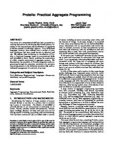
(b e1 . . . en ) (f e1 . . . en ) e ::= ;; expression x l (rep x w e) (nbr e) (if e e e) ;; special constructs w ::= x l ;; variable or value F ::= (def f(x1 . . . xn ) e) ;; function P ::= F1 . . . Fn e ;; program Fig. 1. Field calculus syntax, expressed in modified BNF

it can approximate any causal and approximable space-time computation, discrete or continuous [2]. We here provide an informal account of its semantics. Field calculus is based on five constructs, combined according to the syntax in Figure 1. The basic element of field calculus is an expression e specifying a field computation— since the calculus is functional e also expresses the result of one such computation. The terminal expressions are literals l mapping all points to a data value l such as a number or Boolean, and variables x referencing a function parameter or rep state variable as defined below. These are then composed using the following five constructs: • Built-in operators: A built-in operator b determines the value of its output field at event m (a point in spacetime) only from the values of the environment e and input fields e1 , e2 , . . . at m. The built-in operators can range over any such functions, including addition, comparison, sensors, actuators, etc. • Function definition and call: Abstraction and recursion are supported by function definition: functions are declared Lisp-style with expressions of the form (def f(x1 . . . xn ) e) and applied by expressions of the form (f e1 . . . en ). • Time evolution: Program state is initialized and changed over time by a “repeat” construct (rep x w e). The state variable x is initialized to a literal or variable and updated at each step by computing e against the prior value of x. • Neighborhood values: The (nbr e) construct obtains a field mapping neighboring devices to their most recent available value of e. For example, (min-hood (nbr e)) maps each device to the minimum value of e amongst its neighbors (excluding itself). These can then be manipulated and summarized with built-in operators. Note that the notion of neighbourhood is typically application specific, e.g., given by wireless proximity. • Domain restriction: Distributed branching is implemented by (if e0 e1 e2 ), which computes e1 where e0 is true and e2 where e0 is false by restricting the environment domain. This prevents computations from spreading unexpectedly and allows termination of recursion.1 A field calculus program is then a set of function definitions followed by an expression to be evaluated, distributed for simultaneous unsynchronized execution on every device in the network. For example, field calculus can be used to compute distance to high temperatures with: 1 Domain restriction is quite important for predictable composition of distributed algorithms, but is currently supported by surprisingly few distributed programming models.

(def distance-to (source) (rep d infinity (mux source 0 (min-hood (+ (nbr d) (nbr-range)))))) (distance-to (> (temperature) 25))

It uses four built-in operators: temperature extracts temperature from the environment state, nbr-range determines the most recent distance to an event’s neighboring devices, + applies addition point-wise over fields, and mux multiplexes between its second and third inputs, returning the second if the first is true and the third otherwise. For full details of field calculus, its semantics, and more examples, see [1]. In defining our building block operators, we will also assume an extension of field calculus to a simple form of firstclass functions. In particular, we make some of our constructs more generic by allowing metrics and reduction functions to be passed as a named or anonymous function (via a fun construct otherwise identical to def). This use, however, may be considered as syntactic sugar for expressing a family of closely related constructs, rather than an actual change in semantics. B. Self-Stabilisation Self-stabilisation [16] is a property of an algorithm such that, beginning from any arbitrary state, the algorithm is guaranteed to return to a legal state within finite time. This is the robust execution property that we will obtain for all of our building block algorithms. Importantly, given any set of self-stabilising algorithms that converge to a fixed state, all “feed-forward” functional compositions of such algorithms are themselves self-stabilising [3]. Intuitively, this can be understood as follows: if the inputs of such an algorithm stop changing, then its output will self-stabilise and stop changing. Then any algorithm that consumes its output will have an input that stops changing, and eventually all algorithms will have come to a stationary point. Thus, we can be ensured that all distributed systems constructed of our building blocks will be guaranteed to be self-stabilising. III. TAXONOMY Inspired by the approach of combinatory logic [17], the catalog of self-organisation primitives in [18], and the simple self-stabilising calculus in [3], the main goal of this paper is to provide a set of building blocks, in the form of a library of functions defined in terms of the field calculus above, to be combined to create advanced applications involving aggregate programming of collective systems. Complex computations over fields will then be structured as a functional combination of these building blocks: apart from locally computable functions (which involve neither communication nor memory and are applied event-wise to a field), they will range over a finite and small set, as described in detail in next section. Here, we sketch a taxonomy of such building blocks that justifies their adoption, and paves the way towards a more formal understanding of issues related to expressiveness, completeness,

Function Structure Aggregation Spreading Symmetry breaking Restriction Compute

Space Time nbr-range,. . . dt,. . . C T G S random if local functions, random

Fig. 2. Taxonomy and proposed building blocks

Computation — This last category contains all “local” functions that do not meaningfully interact with space or time, such as logical and mathematical operations. In next section we shall pick, describe and put to practice a collection of algorithmic building blocks covering the above categories, per Figure 2, describing in detail all with non-trivial implementations in field calculus. •

IV. B UILDING B LOCK O PERATORS and universality. As an additional design criterion, we shall consider only building blocks enjoying the self-stabilisation property, as a means to ensure a more thorough understanding of the result of computation, and ultimately, easier to predict system behaviors. A first key taxonomic distinction is between space and time. Space and time are two complementary dimensions in field computations, the interplay of which regulate the complex dynamics of collective systems. Although space and time are often entangled, some constructs are best understood in terms of space, others time, and others cross both (e.g., local functions, which have no dependencies across space or time). Our second taxonomic distinction is the “function” played by the construct, namely, its role in achieving the desired selforganised behaviour. We identify as one general computation pattern for aggregate systems the following “cycle”: (i) devices monitor their environment for signals of interest (e.g., current temperature), (ii) signals are combined to detect situations of interest (e.g., is average temperature in a region above a threshold?), (iii) information about the situation must move towards the devices(s) able to act (e.g., temperature alert sent to refrigeration units), and finally, (iv) the system acts in response to the situation (e.g., switch on refrigeration). To perform the above operations we identify six classes of operations (each possibly working in space or time): • Structure — Building blocks related to structure yield significant information about the physical environment in which the system operates, mostly in term of its spatial structure: they are provided as 0-ary functions yielding a field of information provided by an environmental sensor. • Aggregation — A key element of aggregate programming is the ability to collect information from across space and time and construct a summary of the situation. Functions implementing aggregation are typically fed with fields describing what we aggregate, where and how. • Spreading — Information from a particular location often needs to be moved to other devices that need to be aware of it. Functions implementing spreading are typically fed with fields describing what information is spread, from where, to where, and how information is possibly modified as it spreads. • Symmetry breaking — These functions have the goal of identifying a limited set of space-time locations where/when an action is to be taken. • Restriction — Restriction splits space-time into subregions so as to possibly carry on different computations in each: this controls the scope of a distributed computation.

We now discuss in detail a set of building block operators covering our taxonomy (except local functions and measurements, which are defined as typical for any language). For each building block, we describe its operation, sketch a proof of self-stabilisation, and discuss applications. To emphasize use of building block operators, we color them (and close derivatives) blue in code samples; field calculus keywords are red and built-in functions green. A. G: Spreading Information Across Space We begin with the G operator, which spreads information across space, potentially further organising and computing as it proceeds. This operator is a generalisation that covers two of the most commonly used self-stabilising distributed algorithms—distance estimation (also often called “gradient”) and broadcast—as well as a number of other applications, such as forecasting along paths. We define the G operator with the following field calculus expression: (def G (source initial metric accumulate) (2nd ;; Return the reduction, discarding the computed distance (rep distance-value (tuple infinity initial) ;; Initial value (mux source (tuple 0 initial);; Source is distance zero, initial value (min-hood ;; Minimize lexicographically over non-self nbrs (tuple (+ (1st (nbr distance-value)) (metric)) (accumulate (2nd (nbr distance-value)))))))))

where min-hood takes the minimum of all neighbors’ values (excluding the device itself), nbr-range returns a field of distances to neighbors, and mux multiplexes between its second and third inputs, returning the second if the first is true and the third otherwise. The G operator may be thought of as executing two tasks, coupled together by the state tuple of distance and value in the rep expression. The first task is computation of a field of shortest-path distances from a source region (indicated as a Boolean field) via the triangle inequality, where distance is computed by the supplied function metric. The second task is computing an accumulation of values along the gradient of the distance field away from the source. This is performed using a function accumulate of one argument, the current accumulated value, beginning with initial value initial. Assuming metric is a valid metric function, distance computation by the triangle inequality is known to selfstabilize [19], either to a correct set of distance estimates (for any connected component containing a source device) or to all values continuously rising toward infinity (for components with no source device). Given a stable set of distance

estimates, the accumulation will self-stabilize as well, since it is continuously refreshed outward from the source (when there is no source, the value is ill-defined and may be neglected). The G operator can be configured to provide a number of different useful services. For example, shortest-path distances can be returned by: (def distance-to (source) (G source 0 nbr-range (fun (v) (+ v (nbr-range)))))

and maximum-likelihood path probabilities are returned by: (def max-likelihood (source p) (G source 1 (fun () (* (nbr-range) (- (log p)))) (fun (v) (* v (exp p (nbr-range))))))

while values can be broadcast from the source using: (def broadcast (source value) (G source value nbr-range identity))

and forecasts of obstacles along a path can be made using: (def path-forecast (source obstacle) (G source 0 nbr-range (fun (v) (or v obstacle))))

Note that if there are multiple source devices, they will form a Voronoi partition [20] of the network, each controlling the values on the portion of the network that is closest to itself according to metric. B. C: Collecting Information From Across Space The C operator is complementary to the G operator: whereas G spreads information away from the source, C accumulates information. In order to be maximize orthogonality with G, C assumes it is supplied with a potential field directing the accumulation of information. It may thus be defined: (def C (potential accumulate local null) (rep v local (accumulate local (accumulate-hood accumulate (mux (= (nbr (find-parent potential)) (uid)) (nbr v) null)))))

where uid returns a unique identifier for each device, accumulate-hood uses the function in its first argument to combine values from the field in its second argument, and the find-parent function is defined as: (def find-parent (potential) (mux (< (1st (min-hood (nbr potential))) potential) (2nd (min-hood (nbr (tuple potential (uid))))) NaN))

Here potential is the potential field up which the values of local should be accumulated, combining values with accumulate, which must be a commutative and associative function of two arguments. In order to avoid multiply-counting devices (for those accumulations that are not idempotent), some neighbors are ignored, and their values replaced by a null that must not affect the accumulated value. The C operator is self-stabilising because it continually refreshes its computation: if the potential field is stable, then the set of parents will stabilize as well, into a collection of trees with their roots at local minima of the potential function. On such a tree, the leaves are all set to local each round; from

there, the values propagate inductively to the root, stage by stage, thus ensuring convergence to a consistent set of values. Combining with G (or G-derived functions), we can obtain a general “summary” operator that aggregates the values of a region to a sink and then spreads it throughout space: (def summarize (sink accumulate local null) (broadcast sink (C (distance-to sink) accumulate local null)))

This operator can then be put to a variety of uses, such as averaging values over a region: (def average (sink value) (/ (summarize sink + value 0) (summarize sink + 1 0)))

computing an integral: (def integral (sink value) (summarize sink + (* value (/ 1 (density)))))

or finding the maximum value: (def region-max (sink value) (summarize sink max value))

C. T: Summarising Information Across Time As C and G are for space, the T operator is for time. Since time is one-dimensional, however, there is no distinction between spreading and collecting, and thus there is only need for a single operator. We define the T operator as: (def T (initial decay) (rep v initial (min initial (max 0 (decay v)))))

where decay is a function strictly decreasing the value of its input. This operator may thus be understood as a flexible count-down toward zero, where the rate of the count-down may change over time. Assuming decay is valid, it self-stabilizes in a single round, since its value is always constrained to the range of [0, initial] and any strictly decreasing series of values is a valid behaviour. Example applications of T include timers: (def timer (length) (T length (fun (t) (- t (dt)))))

and time-limited memory: (def limited-memory (value timeout) (2nd (T (tuple timeout value) (fun (t) (tuple (- (1st t) (dt)) (2nd t))))))

where dt returns the elapsed time since the last round. D. S: Sparse Spatial Choice The S operator breaks symmetry by exploiting another frequently used self-organisation principle, mutual inhibition. Devices compete against one another to become local “leaders,” resulting in a random Voronoi partition with a characteristic component size grain. This operator can be implemented as: (def S (grain metric) (break-using-uids (random-uid) grain metric)) (def random-uid () (rep v (tuple (rnd 0 1) (uid)) (tuple (1st v) (uid)))) (def break-using-uids (uid grain metric)

(= uid (rep lead uid (distance-competition (G (= (uid) lead) 0 metric (fun (v) (+ v (metric)))) lead uid grain metric)))) (def distance-competition (d lead uid grain metric) (mux (> d grain) uid (mux (>= d (* 0.5 grain)) infinity (min-hood (mux (>= (+ (nbr d) (metric)) (* 0.5 grain)) infinity (nbr lead))))))

First each device picks a random identifier, ensuring lack of collisions by adding the device unique identifier as a second element of the UID. Refreshing the device identifier each round ensures this is self-stabilising. These UIDs are then used to break symmetry by a competition between devices for leadership: candidate leader devices surrender leadership to the lowest nearby UID (measuring distance with metric and G). In the case where no device nearby is a leader, devices nominate themselves. The S operator self-stabilizes differently from the other operators, possibly converging to any set of lead devices giving an appropriate cover of the network. Self-stabilisation depends on the flexibility in the placement of lead devices, and can be shown inductively from the dominance of the lead candidate with the lowest UID. The S operator is useful for partitioning and for finding sets of “representative” devices. For example, it can be used to designate a representative device in a sensor network to act as a collection point and relay to the consumers of the network’s sensor data. E. Restriction in Space Finally, in addition to the operators for creating patterns that we have considered thus far, we have spatial restriction of a computation by means of the field calculus if construct. This operator is not new (it was originally introduced in [10]), but it is a critical tool for composition. In essence, the value of if is that it allows one part of a distributed system to modulate the behaviour of another part without a direct connection between their code, by modifying where the code can run. For example, we can use it to navigate around obstacles: (def distance-avoiding-obstacles (source obstacles) (if obstacles infinity (distance-to source)))

or to broadcast only within a particular region: (def broadcast-region (region source value) (if region (broadcast source value) NaN))

to measure the size of connected components of a region: (def group-size (region) (if region (summarize (S (diameter)) + 1 0) NaN))

or to remember whether an event has recently occurred: (def recent-event (event timeout) (if event true (> (timer timeout) 0)))

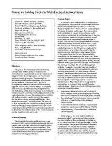
Fig. 3. Composite snapshot of simulation of crowd tracking and warning for a crowded event in Boston’s Columbus Park. Dangerously crowded areas are marked in red, nearby alerted devices marked in orange, dense but nondangerous crowds marked in blue, and other devices are grey, as are links c between devices. Map OpenStreetMap.

V. A PPLICATION E XAMPLE To illustrate the efficacy of the proposed building blocks, we consider their use in an example complex application scenario. In particular, we consider the problem of crowd management and safety in large public events such as concerts, festivals, and sports matches. In such circumstances, emergent dynamics in the location and behaviour of people frequently cause some areas of space to become dangerously overcrowded. In such critical conditions, any small incident may—and often does— create a tragedy with many people killed and injured [21]. Crowding is often evaluated by a notion of “level of service” expressed in terms of density of pedestrians [22]. At a critical density a little more than two people per square meter, crowds typically transition from dense but flowing to congested and potentially dangerous. In a crowd of people carrying smart phones or similar devices, the instantaneous local crowd density could be estimated by device-to-device interaction (e.g., via low-energy Bluetooth). Assuming such a measure is available, we can build a crowd-tracking algorithm that identifies areas of dangerous crowding. This can be done using only the proposed building blocks (along with local functions the derived functions provided in the previous section): (def crowd-tracking (p) ;; Consider only devices experiencing Fruin LoS E or F within last minute (if (recently-true (> (density-est p) 1.08) 60) ;; Use S to break into ‘‘cells’’ and estimate danger of each (+ 1 (dangerous-density (S 30) p)) 0)) (def recently-true (state memory-time) ;; Make sure first state is false, not true... (rt-sub (not (timer 1)) state memory-time)) (def rt-sub (started state memory-time) (if state true (limited-memory started memory-time))) (def dangerous-density (partition p) ;; Only dangerous if above critical density threshold... (and (> (average partition (density-est p)) 2.17)

;; ... and also involving many people. (> (summarize partition + (/ 1 p) 0) 300)))

where p is the fraction of people’s devices participating in the algorithm. This algorithm assigns every device to a class of 2 if it is dangerously crowded, 1 if it is dense but not dangerous, and 0 if uncrowded. With such a crowd estimate, we can then add crowd safety and management layers, such as sending an alert notice to anyone in or near a dangerously crowded area: (def crowd-warning (p range) (> (distance-to (= (crowd-tracking p) 2)) range))

Figure 3 shows an example of crowd-warning and crowd-tracking for a hypothetical scenario of a large festival in Boston’s waterfront Columbus Park, simulated using MIT Proto [10]. In this simulation, 650 devices represent 10% of attendees running the crowd management application on their phones (p=0.1), devices communicate with neighbors up to 15 meters under a unit disc model, and warnings are distributed to a range of 30 meters. A waterfront attraction has caused people to pack against the shore, concentrating dangerously in one corner of the pier, and another attraction is causing potentially dangerous congestion near an intersection of footpaths. As can be seen, the program identifies crowds, distinguishes those large and dense enough to potentially be dangerous, and warns people who are nearby. Other examples of crowd management services that could be implemented very simply using these primitives include navigation avoiding dense crowds: (def safe-navigation (destination p) (distance-avoiding-obstacles destination (crowd-warning p)))

and recommendations to help people disperse safely from an overcrowded environment: (def safe-dispersal (p) (distance-to (= (crowd-tracking p) 0)))

VI. C ONTRIBUTIONS This paper has presented a collection of “building block” algorithms for complex distributed applications, thereby raising the abstraction level at which device aggregates can be programmed. These algorithms are derived from commonly used self-organisation mechanisms, and have the property that both the individual algorithms and all legal compositions thereof exhibit predictable self-stabilising behaviour. To the best of our knowledge, this is the first such catalog of general and composable self-organisation mechanisms. This work thus represents an important step towards the ultimate goal of making distributed systems as simple to engineer as individual computers. In future work, it will be important to establish additional properties for robust execution properties, most particularly in adjusting algorithms to ensure that they tolerate heterogeneity in network density and to ensure good behaviour during as well as after self-stabilisation. Likewise, the catalog of useful primitives is by no means complete. Future research will thus also need to broaden the collection of building block algorithms while continuing to ensure their safe and predictable composition.

ACKNOWLEDGMENT Thanks to Danilo Pianini and Kyle Usbeck for useful discussions and feedback regarding the building block operators. R EFERENCES [1] M. Viroli, F. Damiani, and J. Beal, “A calculus of computational fields,” in Advances in Service-Oriented and Cloud Computing, ser. Communications in Computer and Information Sci., C. Canal and M. Villari, Eds. Springer Berlin Heidelberg, 2013, vol. 393, pp. 114–128. [2] J. Beal, M. Viroli, and F. Damiani, “Towards a unified model of spatial computing,” in 7th Spatial Computing Workshop (SCW 2014), AAMAS 2014, Paris, France, May 2014. [3] M. Viroli and F. Damiani, “A calculus of self-stabilising computational fields,” in 16th Conference on Coordination Languages and Models (Coordination 2014), Jun. 2014, pp. 163–178. [4] F. Zambonelli, G. Castelli, L. Ferrari, M. Mamei, A. Rosi, G. D. M. Serugendo, M. Risoldi, A.-E. Tchao, S. Dobson, G. Stevenson, J. Ye, E. Nardini, A. Omicini, S. Montagna, M. Viroli, A. Ferscha, S. Maschek, and B. Wally, “Self-aware pervasive service ecosystems,” Procedia CS, vol. 7, pp. 197–199, 2011. [5] R. Gummadi, O. Gnawali, and R. Govindan, “Macro-programming wireless sensor networks using kairos.” in Distributed Computing in Sensor Systems (DCOSS), 2005, pp. 126–140. [6] M. P. Ashley-Rollman, S. C. Goldstein, P. Lee, T. C. Mowry, and P. Pillai, “Meld: A declarative approach to programming ensembles,” in IEEE Intelligent Robots and Systems (IROS), 2007, pp. 2794–2800. [7] S. Madden, M. Franklin, J. Hellerstein, and W. Hong, “Tinydb: An acqusitional query processing system for sensor networks,” in ACM TODS, 2005. [8] R. D. Nicola, G. Ferrari, M. Loreti, and R. Pugliese, “A language-based approach to autonomic computing,” in Formal Methods for Components and Objects, ser. LNCS, vol. 7542, 2013, pp. 25–48. [9] J. Beal, S. Dulman, K. Usbeck, M. Viroli, and N. Correll, “Organizing the aggregate: Languages for spatial computing,” in Formal and Practical Aspects of Domain-Specific Languages: Recent Developments, M. Mernik, Ed. IGI Global, 2013, ch. 16, pp. 436–501. [10] J. Beal and J. Bachrach, “Infrastructure for engineered emergence on sensor/actuator networks,” IEEE Intelligent Systems, vol. 21, no. 2, pp. 10–19, 2006. [11] M. Mamei and F. Zambonelli, “Programming pervasive and mobile computing applications: The tota approach,” ACM Trans. on Software Engineering Methodologies, vol. 18, no. 4, pp. 1–56, 2009. [12] R. Newton and M. Welsh, “Region streams: Functional macroprogramming for sensor networks,” in First International Workshop on Data Management for Sensor Networks (DMSN), Aug. 2004, pp. 78–87. [13] M. Viroli, M. Casadei, S. Montagna, and F. Zambonelli, “Spatial coordination of pervasive services through chemical-inspired tuple spaces,” ACM Transactions on Autonomous and Adaptive Systems, vol. 6, no. 2, pp. 14:1 – 14:24, June 2011. [14] M. Mamei and F. Zambonelli, “Self-maintained distributed tuples for field-based coordination in dynamic networks,” Concurrency and Computation: Practice and Experience, vol. 18, no. 4, pp. 427–443, 2006. [15] S. Montagna, M. Viroli, J. L. Fernandez-Marquez, G. Di Marzo Serugendo, and F. Zambonelli, “Injecting self-organisation into pervasive service ecosystems,” Mobile Networks and Applications, vol. 18, no. 3, pp. 398–412, 2013. [16] S. Dolev, Self-Stabilization. MIT Press, 2000. [17] H. B. Curry, Combinatory Logic. North-Holland Pub. Co., 1958. [18] J. Fernandez-Marquez, G. Marzo Serugendo, S. Montagna, M. Viroli, and J. Arcos, “Description and composition of bio-inspired design patterns: a complete overview,” Natural Computing, vol. 12, no. 1, pp. 43–67, 2013. [19] J. Beal, J. Bachrach, D. Vickery, and M. Tobenkin, “Fast self-healing gradients,” in Proceedings of ACM SAC 2008, 2008, pp. 1969–1975. [20] F. Aurenhammer, “Voronoi diagrams: a survey of a fundamental geometric data structure,” ACM Computing Surveys, vol. 23, no. 3, pp. 345–405, 1991. [21] G. K. Still, Introduction to Crowd Science. CRC Press, 2014. [22] J. Fruin, Pedestrian and Planning Design. Metropolitan Association of Urban Designers and Environmental Planners, 1971.